Estimating snow depth on Arctic sea ice using satellite microwave radiometry and a neural network - The Cryosphere
←
→
Page content transcription
If your browser does not render page correctly, please read the page content below
The Cryosphere, 13, 2421–2438, 2019
https://doi.org/10.5194/tc-13-2421-2019
© Author(s) 2019. This work is distributed under
the Creative Commons Attribution 4.0 License.

Estimating snow depth on Arctic sea ice using satellite
microwave radiometry and a neural network
Anne Braakmann-Folgmann and Craig Donlon
European Space Agency, Keplerlaan 1, 2201AZ Noordwijk, the Netherlands

Correspondence: Anne Braakmann-Folgmann (anne.bf@gmx.de)

Received: 12 March 2019 – Discussion started: 28 March 2019
Revised: 30 July 2019 – Accepted: 15 August 2019 – Published: 17 September 2019

Abstract. Snow lying on top of sea ice plays an important         show that both our neural networks outperform the other al-
role in the radiation budget because of its high albedo and       gorithms in terms of accuracy, when compared to the OIB
the Arctic freshwater budget, and it influences the Arctic cli-   data and we demonstrate that plausible results are obtained
mate: it is a fundamental climate variable. Importantly, ac-      even outside the algorithm training period and area. We then
curate snow depth products are required to convert satellite      convert CryoSat freeboard measurements to SIT using dif-
altimeter measurements of ice freeboard to sea ice thickness      ferent snow products including the snow depth from our net-
(SIT). Due to the harsh environment and challenging acces-        works. We confirm that a more accurate snow depth product
sibility, in situ measurements of snow depth are sparse. The      derived using our neural networks leads to more accurate es-
quasi-synoptic frequent repeat coverage provided by satellite     timates of SIT, when compared to the SIT measured by a
measurements offers the best approach to regularly monitor        laser altimeter at the OIB campaign. Our network with addi-
snow depth on sea ice. A number of algorithms are based           tional SMOS input yields even higher accuracies, but has the
on satellite microwave radiometry measurements and simple         disadvantage of a larger “hole at the pole”. Our neural net-
empirical relationships. Reducing their uncertainty remains       work approaches are applicable over the whole Arctic, cap-
a major challenge.                                                turing first-year ice and multi-year ice conditions throughout
   A High Priority Candidate Mission called the Copernicus        winter. Once the networks are designed and trained, they are
Imaging Microwave Radiometer (CIMR) is now being stud-            fast and easy to use. The combined AMSR2 + SMOS neural
ied at the European Space Agency. CIMR proposes a coni-           network is particularly important as a precursor demonstra-
cally scanning radiometer having a swath > 1900 km and in-        tion for the Copernicus CIMR candidate mission highlight-
cluding channels at 1.4, 6.9, 10.65, 18.7 and 36.5 GHz on the     ing the benefit of CIMR.
same platform. It will fly in a high-inclination dawn–dusk or-
bit coordinated with the MetOp-SG(B). As part of the prepa-
ration for the CIMR mission, we explore a new approach to
retrieve snow depth on sea ice from multi-frequency satel-        1   Introduction
lite microwave radiometer measurements using a neural net-
work approach. Neural networks have proven to reach high          Climate change and globalization are the dominant drivers
accuracies in other domains and excel in handling complex,        of societal impacts in the Arctic with economic develop-
non-linear relationships. We propose one neural network that      ment rapidly transforming the geopolitics and the physical
only relies on AMSR2 channel brightness temperature data          and biogeochemical environment of the region. For example,
input and another one using both AMSR2 and SMOS data              new prospectors are increasing their activities using modern
as input. We evaluate our results from the neural network ap-     techniques for oil and gas, fisheries, and mineral resources,
proach using airborne snow depth measurements from Oper-          and commercial ship traffic is growing dramatically. In this
ation IceBridge (OIB) campaigns and compare them to prod-         context, snow depth is an important parameter for climate
ucts from three other established snow depth algorithms. We       studies, modelling and forecasting. Snow on sea ice strongly
                                                                  influences the Earth’s radiation budget with its high albedo

Published by Copernicus Publications on behalf of the European Geosciences Union.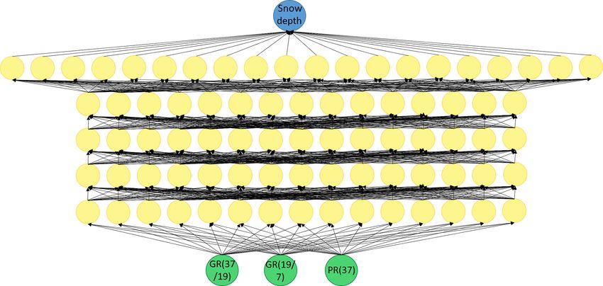
2422                  A. Braakmann-Folgmann and C. Donlon: Estimating snow depth on sea ice with a neural network

and behaves like an insulation controlling sea ice growth and     general the use of microwave radiometer data is limited to
melt. In the melt season snow on sea ice contributes to the       cold and dry snow conditions because in the melt season wet
freshwater input and inhibits deep ocean circulation because      snow acts as a blackbody (Markus et al., 2006).
of surface freshwater stratification. Additionally, to retrieve      Recently it was argued that the use of lower frequencies
sea ice thickness (SIT) from laser (NASA ICESat) or radar         (e.g. 6.9 GHz) that measure microwave emissions deeper in
altimeter (e.g European Space Agency (ESA) CryoSat) free-         the snow layer could improve the accuracy and allow the re-
board measurements, snow depth has to be known with a             trieval of larger snow depths since the 36.5 GHz signal is sat-
high accuracy. The uncertainty in today’s snow on sea ice         urated at around 50 cm (Markus et al., 2006). Rostosky et al.
products contributes significantly to the uncertainty in SIT      (2018) proposed such an algorithm using the gradient ratio
(Zygmuntowska et al., 2014; Giles et al., 2007). Ship traffic     between 6.9 and 18.7 GHz. Furthermore their algorithm en-
across the Northern Sea Route in the Arctic is increasing and     ables an extension to MYI by using two separate empirical
will further increase as sea ice retreats. To navigate through    fits for FYI and MYI.
the sea ice, SIT is a key parameter, but also the snow depth         More recently, Kilic et al. (2019) make use of the low-
itself is relevant due to its very high friction (Huang et al.,   frequency 6.9 GHz channel, but instead of using the gradient
2018).                                                            ratio, they fit a multilinear regression between microwave ra-
   To derive SIT from CryoSat freeboard the Warren clima-         diometer data and snow depth using data from ice mass bal-
tology product (Warren et al., 1999) is often used. It relies     ance (IMB) buoys in the Arctic.
on snow depth measurements collected from manned drift-              In general microwave radiometer observations are widely
ing stations and isolated locations (reached via aircraft) over   used input data for snow depth retrieval. They benefit from a
multi-year ice (MYI) in the Arctic between 1954 and 1991.         long data record, allow at least daily coverage over the poles,
These measurements are summarized in monthly maps and             and most importantly are independent of weather and dark-
contour lines of snow depth have been derived. For lack of        ness. The only drawback is the rather broad spatial resolution
a better operational product, this climatology is still widely    (AMSR2 has a 35 km × 62 km footprint at 6.9 GHz). The Eu-
used – sometimes with a modification factor of 0.5 or 0.7 to      ropean Space Agency (ESA) is now studying a High Priority
account for lower snow depths on first-year ice (FYI) and the     Candidate Mission (HPCM) called the Copernicus Imaging
fact that less ice survives each summer (Kurtz and Farrell,       Microwave Radiometer (CIMR; Donlon and CIMR Mission
2011; Kwok and Cunningham, 2015). Obvious drawbacks of            Advisory Group, 2019). CIMR proposes a conically scan-
this climatology are that it is outdated (Kern et al., 2015),     ning radiometer having a swath > 1900 km and will include
that it was collected mostly over MYI, its quite broad spa-       channels at 1.4 GHz (60 km), 6.9 and 10.65 GHz (< 15 km),
tial resolution and that it does not allow for any interannual    18.7 GHz (5–6 km), and 36.5 GHz (4–5 km) on the same plat-
variation.                                                        form. The mission will occupy a high-inclination dawn–dusk
   The quasi-synoptic frequent repeat coverage provided by        orbit coordinated with the MetOp-SG(B) satellite offering
satellite measurements offers an excellent approach to reg-       opportunities for synergy with the microwave imager (MWI)
ularly monitor snow depth on sea ice. Satellite microwave         and scatterometer (SCA). CIMR would not only guaran-
measurements offer a clear advantage over visible or thermal      tee continuity in microwave radiometer observations, but it
infrared techniques because they penetrate through clouds         would also ensure continuity at the low-frequency L band
and deliver measurements during the long polar night. Un-         (1.4 GHz), currently provided by ESA’s Soil Moisture and
fortunately, at this time the frequencies of primary interest     Ocean Salinity (SMOS) and NASA’s Soil Moisture Active
(1.4–7.0 GHz) are characterized by a large surface footprint.     Passive (SMAP) satellites, and for the first time provide L-
Measurements made at higher frequency (18–89 GHz) are             band and higher-frequency measurements on the same plat-
used to derive estimates of snow depth on sea ice with vary-      form in a high-inclination orbit.
ing degrees of success. A number of algorithms are based             Maaß et al. (2013) demonstrate the possibility to deter-
on simple empirical relationships to in situ measurements,        mine snow depth from 1.4 GHz brightness temperatures mea-
and reducing the uncertainty in derived snow depth prod-          sured by SMOS. The insulation of the snow cover leads to in-
ucts remains a major challenge. The first algorithm that was      creasing brightness temperatures at 1.4 GHz correlated with
developed using satellite microwave radiometer data is re-        snow depth. Maaß et al. (2013) find that the effect is more
ported in Markus and Cavalieri (1998). It uses an empirical       pronounced at horizontal polarization. The approach works
relation between the gradient ratio of the 37.0 and 19.4 GHz      well for thick sea ice (ice thicker than 1–1.5 m) and snow
channels of the Special Sensor Microwave/Imager (SSM/I)           depths of 35 cm. Also, Zhou et al. (2018) developed a com-
together with in situ and ship observations of snow depth in      bined snow depth and SIT retrieval approach from a com-
Antarctica. Comiso et al. (2003) modified the Markus and          bination of SMOS data with laser altimetry incorporating a
Cavalieri (1998) algorithm coefficients to match the slightly     radiation model.
different frequencies of the Advanced Microwave Scanning             Yet another possibility to determine snow depth is to ex-
Radiometer (AMSR-E) and follow-on AMSR2 mission. This             ploit the different scattering horizons from CryoSat (Ku-
algorithm only produces reasonable results over FYI and in        band) and SARAL/AltiKa (Ka-band) (Guerreiro et al., 2016;

The Cryosphere, 13, 2421–2438, 2019                                                   www.the-cryosphere.net/13/2421/2019/
A. Braakmann-Folgmann and C. Donlon: Estimating snow depth on sea ice with a neural network                                 2423

Lawrence et al., 2018). The same concept may be applied to         2     Methodology
the upcoming overlap of CryoSat and ICESat-2 (Lawrence
et al., 2018). ESA currently also investigates the Coperni-        First we review a few existing algorithms for snow depth
cus polaR Ice and Snow Topography ALtimeter (CRISTAL;              on sea ice calculation from satellite microwave radiometer
Kern et al., 2019) as a High Priority Candidate Mission. If se-    brightness temperatures, before we introduce our own neural
lected, CRISTAL would uniquely offer co-temporal Ku- and           network approach. The neural network somehow builds upon
Ka-band measurements in a high-inclination orbit. In com-          the findings of these more traditional algorithms and will also
parison to microwave radiometer measurements, however,             be compared to them in Sect. 4.
the temporal coverage would be quite low due to the small
nadir-only footprint of the altimeter, although repeat global      2.1    Snow depth from Markus and Cavalieri (1998)
sampling every 10 d is anticipated.
   The opportunity for synergy and inter-calibration between       Markus and Cavalieri (1998) developed the first algorithm to
multi-frequency altimetry (e.g. CRISTAL) and CIMR snow             retrieve snow depth hs on sea ice from passive microwave
depth retrievals over sea ice is obvious. As part of the prepa-    measurements in 1998. The physical basis of their algorithm
ration for the future CIMR mission, we explore a new ap-           is the fact that brightness temperature is sensitive to volume
proach to retrieve snow depth on sea ice from satellite mi-        scattering. The brightness temperature over snow on sea ice
crowave radiometer measurements using a neural network             decreases when snow depth increases or when frequency de-
approach. Neural networks provide a technique to model             creases. They found the highest correlation to Antarctic snow
any complex, non-linear relationship, including the multi-         depth observations with the gradient ratio between 19 and
frequency microwave signal emissions from within a snow            37 GHz brightness temperatures Tb at vertical polarization V :
layer. The application of neural networks for this purpose is
still developing but a few simple attempts exist: Tedesco et al.                            Tbice (37V ) − Tbice (19V )
(2004) apply a simple neural network with one hidden layer         hs [cm] = 2.9 − 782 ·                                .     (1)
                                                                                            Tbice (37V ) + Tbice (19V )
to derive snow depth and snow water equivalent (SWE) on
land. They use the 19 and 37 GHz brightness temperatures at
both polarizations as input.                                       Tbice is the brightness temperature of the ice-covered part
   We build a deeper, more advanced neural network to re-          of the footprint. This correction is important since we are
trieve snow depth on sea ice from satellite microwave ra-          only interested in the change of brightness temperature due
diometer measurements and train our network with Opera-            to snow cover and otherwise the open water part would dom-
tion Ice Bridge (OIB) snow depths (Kurtz et al., 2013) in          inate the signal. It is calculated from
the Arctic. We build on the algorithms by Markus and Cav-
alieri (1998) and Rostosky et al. (2018) using both the “tra-                       Tb (f, p) − (1 − SIC) · TbOW (f, p)
                                                                   Tbice (f, p) =                                       .     (2)
ditional” 36.5/18.7 gradient ratio and the lower-frequency                                          SIC
18.7/6.9 gradient ratio as input together with polarization ra-
tios. We also explore the use of SMOS together with AMSR2          TbOW (f, p) is the open-water tie point for frequency f and
data as input for one of our neural networks. Our neural net-      polarization p and SIC is sea ice concentration. In the equa-
works are applicable over both FYI and MYI ice and no ad-          tions we round the frequency to the nearest integer and in-
ditional ice type product is needed to differentiate between       dicate vertical linear polarization with a V and horizontal
both. Once designed and trained, they are fast and easy to         linear polarization with an H . Originally the two linear re-
use and would also work with future measurements from the          gression coefficients were derived from a fit of SSM/I bright-
CIMR radiometer.                                                   ness temperatures to Antarctic in situ and ship observations.
   We verify our neural network approaches with another            Comiso et al. (2003) updated the algorithm coefficients to
part of the OIB data and compare the results to the snow           fit the slightly different incidence angle and frequencies of
depth algorithms by Markus and Cavalieri (1998), Rostosky          AMSR-E. The same coefficients are also applied for the Arc-
et al. (2018), and Kilic et al. (2019). We also evaluate how       tic and their algorithm is still widely used.
the different snow products influence the SIT retrieval from          The algorithm is limited to dry, cold snow, which is thin-
CryoSat freeboard data.                                            ner than 50 cm and should only be applied over FYI (Markus
   In the next section we summarize the different snow depth       et al., 2006). Instead of the original values, we use the coef-
algorithms used for comparison, introduce our neural net-          ficients from Comiso et al. (2003) as given in Eq. (1), open-
work approach and explain the SIT calculation. In Sect. 3          water tie point values for AMSR2 from Ivanova et al. (2014)
we introduce the data used for training, evaluation and com-       and calculate the SIC with the NASA Team algorithm (Cav-
parison. The results are then shown and discussed in Sect. 4       alieri et al., 1984). To be comparable with the other algo-
before we end with a conclusion.                                   rithms, we ignore the shortcomings of the algorithm over
                                                                   MYI and apply it Arctic-wide anyway. This is also an es-
                                                                   sential requirement when applied in SIT retrieval.

www.the-cryosphere.net/13/2421/2019/                                                       The Cryosphere, 13, 2421–2438, 2019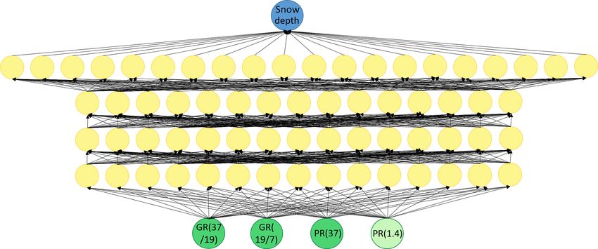
2424                  A. Braakmann-Folgmann and C. Donlon: Estimating snow depth on sea ice with a neural network

2.2    Snow depth from Rostosky et al. (2018)                     They use SIC charts from the European Centre for Medium-
                                                                  Range Weather Forecasts (ECMWF) Re-Analysis Interim
Rostosky et al. (2018) follow a similar approach as Markus        (ERA-Interim) data and discard areas outside 100 % SIC. To
and Cavalieri (1998) using a gradient ratio and two linear        be consistent with the other approaches we use the OSISAF
regression coefficients. However, instead of using the gradi-     SIC product (Lavergne et al., 2019) and discard areas with
ent ratio between 18.7 and 36.5 GHz, they apply the gradi-        SIC lower than 80 %.
ent ratio of 6.9 to 18.7 GHz. The lower frequencies enable a
determination of snow depths exceeding 50 cm (due to mi-          2.4   Snow depth from our neural network approach
crowave emissions emanating from deeper within the snow
at this frequency), where the 36.5 GHz channel becomes sat-       Artificial neural networks are a means of machine learning
urated. Furthermore a simulation by Markus et al. (2006) and      inspired by the human brain to learn higher-order representa-
a correlation analysis by Rostosky et al. (2018) suggest a        tions and perform diverse tasks. In contrast to other machine
stronger relation of snow depth to this gradient ratio. To use    learning techniques, they are designed to extract relevant fea-
this gradient ratio, they determined a new set of regression      tures and their weighting in the model themselves. Deep
coefficients by fitting AMSR-E and AMSR2 brightness tem-          neural networks allow us to learn higher-order representa-
peratures to OIB snow depth. They exclude single years for        tions, tackle more complex problems and outperform other
verification and validation work. Furthermore they extend the     means of machine learning in terms of accuracy (Schmid-
approach to be applicable over both FYI and MYI, while the        huber, 2015). Neural networks can be viewed as a universal
approach of Markus and Cavalieri (1998) was found to de-          system to represent any function. Instead of designing repre-
liver reasonable results only over FYI. The extension to MYI      sentative features or building a complex physical model, the
is achieved by fitting a second set of parameters to the MYI-     challenge with neural networks is to design an appropriate
covered part of the OIB data. We use the coefficients deter-      architecture.
mined with OIB data from 2009 to 2014 since our test data            We design our neural networks with the framework Keras
are from 2015. When applying this algorithm, the ice type         (Chollet et al., 2015), using TensorFlow (Abadi et al., 2015)
(FYI or MYI) must be known with confidence. They use the          back end. Three inputs from AMSR2 are used in our neu-
ice type product from OSISAF – derived by a combination of        ral networks: the gradient ratio between vertically polar-
microwave radiometry and scatterometer data (Aaboe et al.,        ized brightness temperatures at 18.7 and 36.5 GHz, as pro-
2016) – and discard areas where the ice type is not known         posed by Markus and Cavalieri (1998), the gradient ratio be-
with high confidence (confidence level < 4). On FYI snow          tween vertically polarized brightness temperatures at 6.9 and
depth is calculated from                                          18.7 GHz, as used by Rostosky et al. (2018), and the polariza-
                                                                  tion ratio (PR) between vertically and horizontally polarized
                             Tbice (19V ) − Tbice (7V )           brightness temperatures at 36.5 GHz:
hs [cm] = 19.74 − 556.69 ·                              ,   (3)
                             Tbice (19V ) + Tbice (7V )                      Tbice (37V ) − Tbice (37H )
                                                                  PR(37) =                               .                     (6)
and on MYI from                                                              Tbice (37V ) + Tbice (37H )

                             Tbice (19V ) − Tbice (7V )              This polarization ratio is also used to differentiate between
hs [cm] = 18.73 − 376.32 ·                              .   (4)   FYI and MYI by Comiso (2012), so it seems likely that this
                             Tbice (19V ) + Tbice (7V )
                                                                  information is not directly correlated with snow depth, but
   Again, SIC from the NASA Team algorithm is used to cor-        rather with the ice type and that the neural network uses this
rect for the open-water part within the footprint (Eq. 2).        input in a similar manner as the approach by Rostosky et al.
                                                                  (2018), which requires independent ice type information. We
2.3    Snow depth from Kilic et al. (2019)                        also experimented with other combinations and gradient and
                                                                  polarization ratios, as well as using the brightness temper-
Kilic et al. (2019) developed a simple multilinear regression     atures directly as input. This choice yields the best results.
approach using vertically polarized brightness temperatures       Just as Markus and Cavalieri (1998), we also apply a correc-
at 6.9, 18.7 and 36.5 GHz. These three channels were iden-        tion for the open-water part within the footprint, using Tbice
tified as the best predictor combination in a forward selec-      with SIC from the NASA Team algorithm in our gradient and
tion method with the OIB data of 2013. They then derived          polarization ratios (Eq. 2).
the multilinear regression coefficients from a fit of AMSR2          The first (AMSR2-only) neural network consists of five
brightness temperatures with the data from four IMB buoys         fully connected hidden layers with 15 neurons in each of the
(2012G, 2012H, 2012J and 2012L) to yield the following for-       first four hidden layers and 20 neurons in the last hidden layer
mula:                                                             (see Fig. 1 for an illustration). The number of layers and neu-
                                                                  rons was empirically found to work best for this specific set-
hs [cm] =177.01 + 1.75 · Tb (7V )                                 up. A few rules of thumb exist for the design of a good neural
           − 2.80 · Tb (19V ) + 0.41 · Tb (37V ).           (5)   network architecture, but to a large part it is subject to trying

The Cryosphere, 13, 2421–2438, 2019                                                   www.the-cryosphere.net/13/2421/2019/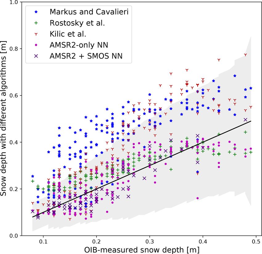
A. Braakmann-Folgmann and C. Donlon: Estimating snow depth on sea ice with a neural network                                             2425

Figure 1. Architecture of the AMSR2-only neural network: the 37/19 gradient ratio, the 19/7 gradient ratio and the polarization ratio at
37 GHz are used as input (green circles). They are transformed by five fully connected hidden layers with 15 or 20 neurons each (yellow
circles) to finally produce snow depth as output (blue circle). Each neuron (circle) has a bias and each connection (arrow) is associated with
a different weight.

different set-ups and observing the error on the validation                 Batch normalization (Ioeffe and Szegedy, 2015) makes a
dataset.                                                                 neural network less sensitive to the random initialization of
   In a fully connected neural network all neurons of the pre-           the weights and biases and improves its generalization ca-
vious layer are connected to each neuron of the next layer               pabilities. The use of batch normalization is recommended
and each connection is associated with a different weight.               for deep neural networks and with sigmoidal non-linearities.
Furthermore each neuron can have a different bias. The out-              Therefore we include batch normalization after the first hid-
put from each neuron in the first hidden layer is given by               den layer.
the sum of all three weights (the arrows connected to this                  Training a neural network means slightly changing its
neuron in Fig. 1) times the three inputs plus the bias of this           weights and biases step by step to minimize a loss function.
neuron. To introduce a non-linearity and enable the network              This technique is known as stochastic gradient descent. The
to learn non-linear relations, the output of each layer may              Adam optimizer (Kingma and Ba, 2015) is a more elabo-
be transformed by a so-called activation function φ. Taking              rate extension of stochastic gradient descent, which we use
into account all 15 outputs from the first hidden layer h we             to train our network in 250 epochs using a batch size of 30.
can write this as a matrix vector multiplication, where W is a           We choose the mean absolute percentage error between the
15 × 3 weight matrix, x the 3 × 1 input vector and b a 15 × 1            estimated snow depth and the OIB snow depth as our loss
bias vector:                                                             function.
                                                                            The design of the second neural network combining
h = φ(W · x + b).                                               (7)      AMSR2 and SMOS input is very similar to the first one. In
                                                                         addition to the three AMSR2 inputs, we add the polarization
   The hidden layers store the features or the information ex-           ratio between vertically and horizontally polarized brightness
tracted from the input. The different weights and biases al-             temperatures at 1.4 GHz from SMOS as a fourth input node.
low each neuron to focus on a different aspect. Usually the              This is calculated analogously to Eq. (6). At 1.4 GHz, SMOS
features get more abstract and complex the deeper the net-               provides a means to penetrate deeper into the snow layer. We
work becomes, since each subsequent layer is created from                also tested gradient ratios between the AMSR2 and SMOS
the already transformed features of the previous layer. The              channels and using brightness temperatures at 1.4 GHz di-
output layer consists of one neuron and represents the esti-             rectly. The polarization ratio gave the best results. This is
mated snow depth.                                                        the only time we do not account for open water within the
   To allow the network to learn non-linear relationships, as            footprint and we do not use open-water tie points to cor-
we expect them to occur in the emission and scattering of a              rect the SMOS brightness temperatures. We calculated some
microwave signal in a snow layer, we apply activation func-              open-water tie points at 1.4 GHz and applied Eq. (2), but this
tions φ. After the first hidden layer we apply a sigmoid func-           slightly degraded the network’s performance, so we choose
tion, after all subsequent hidden layers we apply the rectified          not use them. Because SMOS coverage has a large hole at the
linear unit (ReLU) activation function, and finally the output           pole, we have fewer data for training, validation and testing.
is transformed by a hyperbolic tangent activation function.              Therefore we also reduce the number of parameters of the

www.the-cryosphere.net/13/2421/2019/                                                             The Cryosphere, 13, 2421–2438, 2019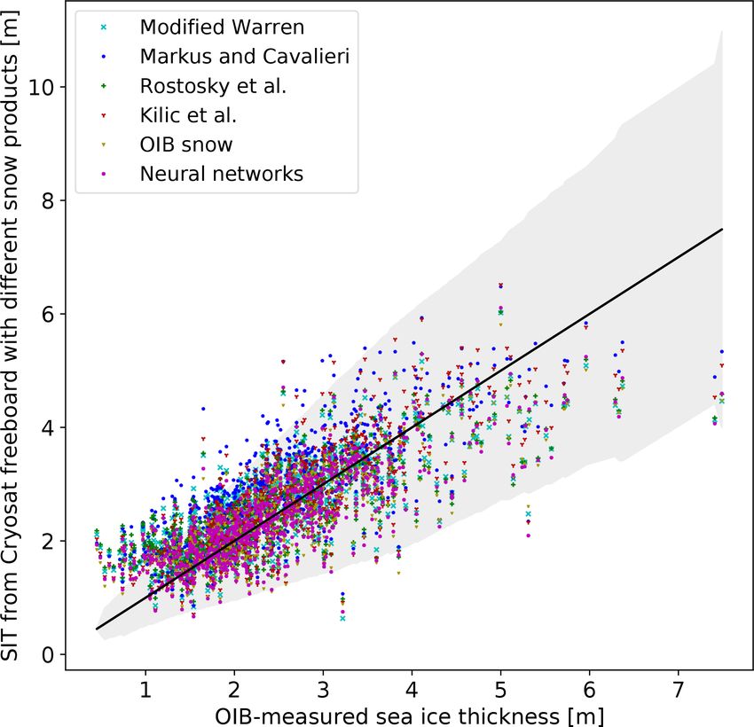
2426                    A. Braakmann-Folgmann and C. Donlon: Estimating snow depth on sea ice with a neural network

Figure 2. Architecture of the AMSR2 + SMOS neural network: the 37/19 gradient ratio, the 19/7 gradient ratio and the polarization ratio at
37 GHz are used as input from AMSR2 (green circles) and the polarization ratio at 1.4 GHz is used as input from SMOS (light green circle).
They are transformed by four fully connected hidden layers with 15 or 20 neurons each (yellow circles) to finally produce snow depth as
output (blue circle).

neural network and delete one hidden layer with 15 neurons.               For the calculation of sea ice freeboard hfb from radar
Otherwise the network is identical to the AMSR2-only net-              freeboard hrfb two corrections should be applied (Kwok,
work. Figure 2 illustrates the design of the combined AMSR2            2014). The first correction δhp accounts for penetration is-
+ SMOS network.                                                        sues caused by the scattering of the Ku-band radar signal at
                                                                       the air–snow interface and within the snow layer. This shifts
2.5    Sea ice thickness                                               the retracking point closer to the satellite. The second correc-
                                                                       tion δhd adjusts the radar freeboard for the slower propaga-
Sea ice thickness (SIT) can be calculated from the sea ice             tion speed of the radar signal within a snow layer:
freeboard hfb measured by CryoSat assuming hydrostatic
equilibrium:                                                           hfb = hrfb + δhp + δhd .                                       (9)
        ρw · hfb + ρs · hs
SIT =                      .                                   (8)        Both corrections have opposite signs and therefore more
             ρw − ρi                                                   or less cancel out depending on the snow depth, the retracker
ρw is the density of seawater, which we set to 1025 kg m−3             and the ratio between the snow–ice and snow–air interface
(Alexandrov et al., 2010), ρi is the ice density and ρs is             peaks (Kwok, 2014). It is especially hard to apply the first
the snow density. For the snow density we assume a bulk                correction since the ratio between the snow–ice and snow–
value of 320 kg m−3 , as suggested by the Warren climatol-             air interface peaks is not known. Kwok’s simulations suggest
ogy (Warren et al., 1999) of March and April (when the                 that for snow depths of 5–30 cm (which covers a major part
OIB data were collected). The ice density depends on the               of the OIB data) both corrections add up to 0.2 cm on average
age of the sea ice and Alexandrov et al. (2010) found a                and are almost independent of snow depth, when a leading
mean value of 882 kg m−3 for MYI and 917 kg m−3 for FYI.               edge retracker is used. Therefore we apply a joint correction
Both values can be weighted according to the MYI fraction              of 0.2 cm to all CryoSat radar freeboard data.
as suggested by Kwok and Cunningham (2015). However,
King et al. (2018) found that using only the MYI value of              3     Data
882 kg m−3 agrees better with helicopter-borne electromag-
netic SIT sounding measurements. We observe the same in                3.1    Operation Ice Bridge (OIB)
comparison to the OIB SIT measurements, and therefore ap-
ply 882 kg m−3 everywhere.                                             Operation Ice Bridge (OIB) was a flight campaign conducted
   The last – and a major – uncertainty in the calculation of          in March and April 2009–2015 by NASA (Kurtz et al.,
SIT is snow depth hs (Zygmuntowska et al., 2014; Giles et              2013). The onboard snow radar provides snow depth mea-
al., 2007). Here we use the original Warren climatology, its           surements by identifying both the air–snow and snow–ice in-
modified version where snow depth is halved over FYI, and              terface within the radar returns. This time difference can then
the algorithms from Markus and Cavalieri (1998), Rostosky              be converted to snow depth, if the snow density is known.
et al. (2018), and Kilic et al. (2019), our neural networks and        Furthermore, a combination of the onboard laser altimeter
also the snow depth measured directly by the OIB snow radar            (tracking the ice + snow freeboard) with snow depth al-
to see how different snow products influence SIT.                      lows the calculation of SIT (Farrell et al., 2012). We use

The Cryosphere, 13, 2421–2438, 2019                                                          www.the-cryosphere.net/13/2421/2019/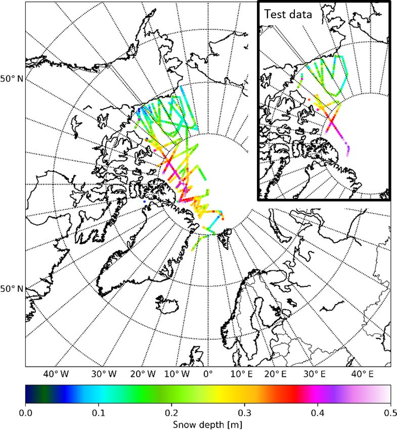
A. Braakmann-Folgmann and C. Donlon: Estimating snow depth on sea ice with a neural network                                 2427

                                                                      To train the networks we temporally divide the OIB data
                                                                   into a training (70 %), a validation (15 %) and a test (15 %)
                                                                   dataset. This is a common splitting in machine learning and
                                                                   ensures enough training data when the overall number of
                                                                   data is small. We also verified that each of the splits con-
                                                                   tains a similar range of snow depth values and that their his-
                                                                   tograms look alike. Figure 3 shows the flight tracks and the
                                                                   measured snow depths from the 2013–2015 campaigns (the
                                                                   overall dataset). The top right box illustrates which parts are
                                                                   used as test data and the snow depth values occurring in this
                                                                   split. We end up with 755 valid snow depth measurements in
                                                                   2013 and 2014 for training, 162 valid measurements in 2014
                                                                   and 2015 for validation – meaning the identification of the
                                                                   best network architecture – and 162 valid snow depth mea-
                                                                   surements in 2015 for testing. When we train the AMSR2 +
                                                                   SMOS neural network, we have to discard all areas (espe-
                                                                   cially the bigger hole at the pole) where no SMOS data are
                                                                   available. Again we split the remaining data into 70 % for
                                                                   training and 15 % for validation and test each and confirm
                                                                   similar histograms of all splits. This gives us only 299 valid
                                                                   data points for training, 64 for validation and 65 for testing.

                                                                   3.2   AMSR2
Figure 3. Flight tracks of the Operation Ice Bridge (OIB) cam-
paigns 2013, 2014 and 2015. The measured snow depth is colour-
coded. The box on the top right shows which part of the OIB data   To train the neural networks and for all comparisons with
are used as test data.                                             OIB data, we use the collocated AMSR2 brightness tem-
                                                                   peratures provided in the RRDP. For all other purposes
                                                                   (longer time series and maps of the whole Arctic), we
OIB data from the Round Robin Data Package (RRDP) ver-             use the AMSR2 L1R brightness temperature swath data
sion 2. This dataset was developed as part of ESA’s sea ice        from JAXA (available at ftp://ftp.gportal.jaxa.jp, last access:
climate change initiative (CCI) project and can be down-           15 August 2018). In the L1R product all frequencies are re-
loaded from http://www.seaice.dk/RRDB-v2/ (last access:            sampled to the 6.9 GHz resolution and centred at the centre of
2 November 2018). It contains the OIB snow depth and SIT           the 89 GHz (A) footprint (Maeda et al., 2016). Since CIMR
data together with collocated AMSR-E or AMSR2 data. In             would provide the same frequencies that we are using (6.9,
this study we only use data from the years 2013–2015, where        18.7 and 36.5 GHz) at the same incidence angle (55◦ ) and
AMSR2 data are available, to avoid the need for an AMSR-E          a similar L1R product, our neural network could directly be
versus AMSR2 inter-calibration. The OIB data in this RRDP          applied to CIMR data and would provide snow depth at a
stem from NSIDC, and OIB snow depth data are averaged              higher spatial resolution.
into 50 km sections for a better overlap and collocation with
AMSR (Pedersen et al., 2019).
                                                                   3.3   SMOS
    The OIB-measured snow depth and SIT were compared
to ground-based in situ measurements along a 2 km transect
from the Danish GreenArc sea ice camp across different ice         We use daily L3 SMOS data from the Centre Aval de Traite-
types. Both snow depth and SIT were found to agree very            ment des Données SMOS (CATDS), available at https://
well with in situ data (mean difference 0.01 and 0.05 m re-        www.catds.fr/sipad/ (last access: 7 January 2019). This prod-
spectively) (Farrell et al., 2012). Also a comparison to in        uct is derived from L1C by gridding it to the 25 km global
situ snow depth measurements from the Bromine, Ozone,              EASE-2 grid. RFI filtering is applied and certain SMOS
and Mercury Experiment (BROMEX; Webster et al., 2014)              L1C flags are taken into consideration. The brightness tem-
and to a reconstruction of snow depth from snowfall reanaly-       peratures are available at full linear vertical and horizontal
sis data and sea ice motion (Blanchard-Wrigglesworth et al.,       polarization and averaged into 5◦ incidence angle bins (Al
2018) shows good agreement. Therefore we regard the OIB            Bitar et al., 2017; Kerr et al., 2013). We average the ascend-
data as the best available validation dataset and use a part of    ing and descending tracks and two of those incidence angle
it to train our neural network and another part for evaluation.    bins to receive brightness temperatures around a 55◦ (50–
                                                                   60◦ ) incidence angle, as CIMR would measure them (Kilic
                                                                   et al., 2018). To collocate the SMOS data with the OIB and

www.the-cryosphere.net/13/2421/2019/                                                    The Cryosphere, 13, 2421–2438, 2019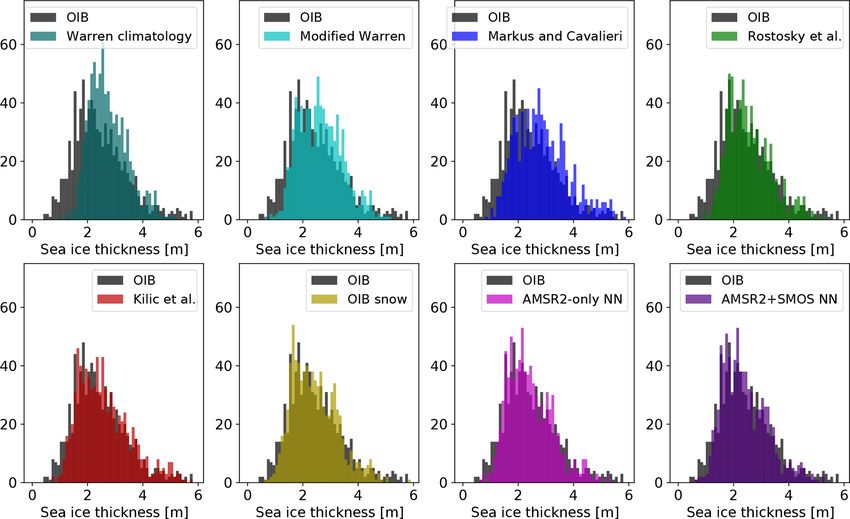
2428                     A. Braakmann-Folgmann and C. Donlon: Estimating snow depth on sea ice with a neural network

AMSR2 data from the RRDP, we average SMOS measure-               4     Results and discussion
ments within 25 km from the OIB position of the same date.
                                                                 4.1     Results on snow depth
3.4     CryoSat
                                                                 4.1.1    Comparison to OIB and other algorithms
For the calculation of SIT, we use the radar freeboard data
in the Geophysical Data Record (GDR) product from the            In this section we measure the performance of our neural net-
CryoSat-2 Science server: http://science-pds.CryoSat.esa.int     works and compare the results to the algorithms proposed
(last access: 4 February 2019). Flagged freeboard data are       by Markus and Cavalieri (1998), Rostosky et al. (2018), and
excluded. To compare the CryoSat-derived SIT with the OIB        Kilic et al. (2019). For this evaluation we employ the test data
SIT, we need to collocate the CryoSat freeboard with the OIB     part of the OIB snow depth measurements. The performance
measurements. For each OIB SIT measurement we average            is evaluated using the root-mean-squared error (RMSE), the
all CryoSat measurements within 25 km from the OIB posi-         correlation coefficient CC, the coefficient of determination
tion and within ±10 d of the OIB flight, assuming that SIT       (R 2 ) and the bias. These are defined as follows:
does not change so quickly. In areas of mixed ice types and                 s
fast sea ice drift this assumption might not hold, but we want                  PN
                                                                                             − yi )2
                                                                                   i=1 (fi
to avoid too many data gaps. Doing so, we take the mean          RMSE =                                ,                    (10)
                                                                                        N
of on average 296 CryoSat freeboard measurements (me-                           PN
dian: 167 CryoSat measurements) and thereby account for                            i=1 (fi  − f¯)(yi − ȳ)
                                                                 CC = qP                                           ,        (11)
the much smaller footprint of CryoSat compared to the snow               N                  ¯  2·
                                                                                                  PN             2
                                                                           i=1  (f  i −  f   )     i=1 (yi − ȳ)
depth products and the averaged OIB data in the RRDP, but
                                                                                              2
                                                                           P
also reduce the uncertainty of a single freeboard measure-                    (y i  −   f i )
                                                                 R 2 = 1 − Pi                   ,                           (12)
ment.                                                                        i (y i   − ȳ)  2
                                                                        PN
3.5     Ancillary data                                                       (fi − yi )
                                                                 bias = i=1                   ,                             (13)
                                                                              N
3.5.1    Ice concentration chart
                                                                 with fi being the estimated values from the algorithm, yi
All snow depth on sea ice algorithms that are investigated       values from OIB and ȳ or f¯ the mean of the OIB or estimated
here rely on a SIC chart to apply them only in areas of at       values respectively.
least 80 % SIC. For this we apply the SIC product from OS-          Table 1 shows the results for the different algorithms. Here
ISAF available at ftp://osisaf.met.no/reprocessed/ice/conc/      we use only those parts of the data where AMSR2, SMOS
v2p0 (last access: 5 December 2018) (Lavergne et al., 2019).     and OIB data are available. This gives us 65 valid data points
Apart from Kilic et al. (2019) all algorithms also require SIC   for testing. In terms of RMSE and the coefficient of deter-
to correct the brightness temperatures for a potential open-     mination, the two neural networks (AMSR2-only NN and
water part within the footprint. For this purpose we apply       AMSR2 + SMOS NN) yield the best results, followed by the
the NASA Team (Cavalieri et al., 1984) algorithm, as sug-        approach by Rostosky et al. (2018). For Markus and Cava-
gested by Markus and Cavalieri (1998). This is much faster       lieri (1998) one should keep in mind that we include snow
than to map a gridded SIC chart to all swath data, but it also   depth estimates over MYI, where the algorithm is known
misidentifies a few areas in the open ocean as sea ice. To re-   to have issues. Concerning the correlation the algorithms by
move these we use the more accurate OSISAF SIC chart at          Rostosky et al. (2018) and Kilic et al. (2019) perform best,
the end.                                                         giving correlation coefficients of 0.93. Last but not least, the
                                                                 neural networks have essentially no bias (0.00 and −0.01 m),
3.5.2    Ice type product                                        while Rostosky et al. (2018) show the second smallest bias
                                                                 with 0.06 m. So overall both neural networks show very
The algorithm from Rostosky et al. (2018) requires reliable      promising results and a higher agreement with OIB snow
information on the ice type to distinguish FYI from MYI.         depth than the other algorithms. Comparing both neural net-
As proposed in their paper, we also use the OSISAF ice type      works with each other, we can easily conclude that the ad-
product (Aaboe et al., 2016) from ftp://osisaf.met.no/archive/   dition of SMOS data further improves the neural network’s
ice/type (last access: 30 October 2018). The same product is     accuracy – only the bias slightly increases.
also used to modify the Warren climatology. In areas of FYI         To also exploit those parts of the OIB data where no SMOS
we halve the original snow depth values.                         data are available, we now show the results on the full OIB
                                                                 test dataset (162 valid data points for testing instead of 65).
                                                                 Figure 3 top right corner shows the whole test dataset from
                                                                 OIB. It covers a range of snow depths on both FYI and MYI.
                                                                 The AMSR2 + SMOS neural network results stem from the

The Cryosphere, 13, 2421–2438, 2019                                                     www.the-cryosphere.net/13/2421/2019/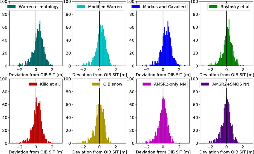
A. Braakmann-Folgmann and C. Donlon: Estimating snow depth on sea ice with a neural network                                      2429

Table 1. RMSE, correlation, coefficient of determination and bias
between the different snow depth retrieval algorithms and OIB-
measured snow depth for all the test data where SMOS data are
available. The best score of each category is highlighted in bold.

                               RMSE      CC        R2        Bias
 Markus and Cavalieri (1998)   0.20 m    0.75    −4.37     0.18 m
 Rostosky et al. (2018)        0.07 m    0.93     0.31     0.06 m
 Kilic et al. (2019)           0.13 m    0.93    −1.33     0.10 m
 AMSR2-only NN                 0.05 m    0.84     0.63     0.00 m
 AMSR2 + SMOS NN               0.04 m    0.91     0.79    −0.01 m

Table 2. RMSE, correlation, coefficient of determination, and bias
between the different snow depth retrieval algorithms and OIB-
measured snow depth for all the test data. When no SMOS data are
available, the neural network with SMOS is equal to the neural net-
work without SMOS. The best score of each category is highlighted
in bold.

                                RMSE       CC       R2       Bias
 Markus and Cavalieri (1998)    0.19 m    0.77    −2.67    0.17 m     Figure 4. OIB-measured snow depth (test data) versus estimated
 Rostosky et al. (2018)         0.07 m    0.90     0.58    0.04 m     snow depth using different algorithms. Note that Markus and Cav-
 Kilic et al. (2019)            0.16 m    0.89    −1.44    0.12 m     alieri (1998) should only be applied over FYI, but this plot also
 AMSR2-only NN                  0.06 m    0.82     0.61    0.00 m     includes MYI.
 AMSR2 + SMOS NN                0.06 m    0.85     0.66    0.00 m

                                                                      when only those parts of the data are used where SMOS data
                                                                      are available. With CIMR we expect to see the same signif-
AMSR2 + SMOS net, if SMOS data are available and from                 icant improvement as demonstrated in Table 1 without the
the AMSR2-only neural network otherwise. This ensures that            problem of losing data for training and testing.
we compare the same part of the data for all approaches and              For a visual impression we plot the estimated snow depth
have more test data available. Combining the two networks             versus the snow depth measured by OIB in Fig. 4. The
could also be useful in a practical application to fill the hole at   black line indicates a perfect match between the algorithm
the pole and to still benefit from higher accuracies in regions       and OIB, and the grey shaded region indicates the uncer-
where SMOS is available. CIMR, however, would cover the               tainty range of the OIB snow depth measurements. In general
whole pole at all frequencies and therefore the AMSR2 +               the neural networks (pink dots for AMSR2-only and purple
SMOS neural network would produce no gaps.                            crosses for AMSR2 + SMOS) and the approach by Rostosky
   Table 2 again shows the results for the different algo-            et al. (2018) (green plus) are closest to OIB. For Markus and
rithms over the whole test dataset. In terms of RMSE and              Cavalieri (1998) (blue stars) we observe that low snow depths
the coefficient of determination, the approach by Rostosky            fit quite well, but larger snow depths are largely overesti-
et al. (2018) and the neural networks again yield the best re-        mated. We acknowledge that these high snow depths prob-
sults (RMSE 0.07, 0.06 and 0.06 m; R 2 0.58, 0.61 and 0.66),          ably occur on MYI, where the algorithm is not well defined.
with the AMSR2-only neural network being slightly better                 Most algorithms start to flatten at around 35–40 cm snow
than Rostosky et al. (2018) and the combined neural network           depth. This behaviour can be explained by the saturation of
working best. Also concerning the correlation here, the al-           the 36.5 GHz signal around this depth. The algorithm by Ros-
gorithms by Rostosky et al. (2018) and Kilic et al. (2019)            tosky et al. (2018) is the only one, solely relying on lower-
outperform the others, giving correlation coefficients of 0.89        frequency channels, and should not yet saturate at this depth.
and 0.90. Last but not least, both neural networks have essen-        Indeed their estimation stays quite close to the OIB measure-
tially no bias (0.00 m), while Rostosky et al. (2018) show the        ments, but also shows a slight decrease in slope. Anyway
second smallest bias with 0.04 m. Overall we can conclude             this might not be significant considering the small number
that the exact excerpt of the data does not make a big differ-        of samples. For the AMSR2 + SMOS neural network, we
ence in terms of the conclusions and here the neural networks         do not observe a flattening, but we also only have very few
also perform best, with the combined neural network outper-           samples available for high snow depth.
forming the AMSR2-only one. The difference between the                   Figure 5 reveals the distribution of OIB snow depth in grey
two neural networks is obviously much larger and clearer,             and the distribution of estimated snow depth in colour. To get

www.the-cryosphere.net/13/2421/2019/                                                        The Cryosphere, 13, 2421–2438, 2019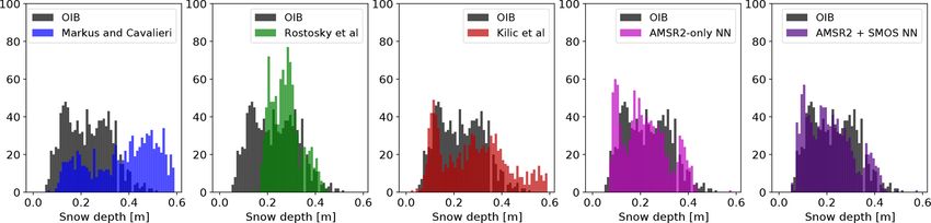
2430 A. Braakmann-Folgmann and C. Donlon: Estimating snow depth on sea ice with a neural network
Figure 5. Distribution of OIB-measured snow depth (all data) in grey versus estimated snow depth using different algorithms in colour.
Figure 6. Deviation from OIB (estimated snow depth using different algorithms minus OIB-measured snow depth) for all OIB data. The
vertical black line indicates a perfect match between OIB and the algorithm, the left half corresponds to an underestimation and the right half
to an overestimation of snow depth compared to the OIB measurements.
a better idea of the algorithms’ characteristics and to be sta- the combined neural network agrees a little bit better with
tistically more meaningful, we show the results for the whole OIB than the AMSR2-only neural network.
OIB dataset. For the test data the plots look similar, but less Finally we also plot the distribution of the deviation from
obvious. For Markus and Cavalieri (1998) (first plot in blue), OIB (estimated snow depth – OIB snow depth) in Fig. 6. The
we again observe that a lot of snow depths are highly overes- vertical black line indicates zero deviation or a perfect match
timated – most likely due to the application of this algorithm between the algorithm and OIB. For clarity, we choose to use
over MYI (where it is poorly constrained). The second plot all the OIB data since the results for the test data look similar.
in green for Rostosky et al. (2018) reveals that this algorithm The neural networks show the least bias and an almost Gaus-
only spans snow depths from around 18 to 45 cm. The over- sian distribution compared to OIB. Their modes are exactly
all agreement is quite good, but the lack of snow depth lower at zero, while all other algorithms tend to more or less over-
than 18 cm is quite striking. The third plot in red is associ- estimate snow depth compared with the OIB measurements.
ated with the snow depth estimates by Kilic et al. (2019).
It reveals the widest spread of estimated snow depth values 4.1.2 Applicability outside the training area and period
and shows a good overall agreement with the OIB distribu-
tion, but a tendency to overestimate snow depth. The plot in To get a better feeling for the algorithms’ performance out-
pink shows the snow depth distribution from our AMSR2- side the areas (west Arctic) and times (spring) of the OIB
only neural network and the purple plot shows the distribu- data, we apply them to the whole Arctic for a whole winter
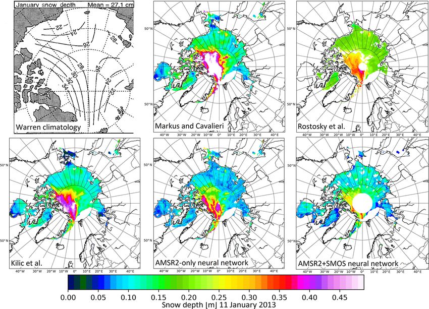
tion from a combination of the two neural networks. When season. Figure 7 shows the spatial distribution of snow depth
SMOS data are available, we use the AMSR2 + SMOS net- on 11 January 2013, gridded to the 25 km EASE2 grid. This
work, otherwise just the AMSR2 network. Both neural net- date was chosen arbitrarily in midwinter. For comparison we
works show the best agreement with OIB: they capture the also include the Warren climatology for January. While we
spread of OIB snow depths quite well just a few snow depths do not know which solution is closest to the truth, we can
deeper than 40 cm are missing and the modes are a little bit see how broad the Warren climatology is compared to the
shifted. A high mode at 10 cm snow depth sticks out in par- maps from satellite data. We also observe that the climatol-
ticular, slightly underestimating OIB snow depth and again ogy only covers the central Arctic. Outside the diagram (e.g.
80◦ N on the Atlantic side) snow depth can only be calcu-
The Cryosphere, 13, 2421–2438, 2019 www.the-cryosphere.net/13/2421/2019/A. Braakmann-Folgmann and C. Donlon: Estimating snow depth on sea ice with a neural network 2431 Figure 7. Map of Arctic snow depth on 11 January 2013 estimated with different algorithms. lated by extrapolation, but is no longer supported by mea- situ snow depth measurements. On FYI our neural networks surements. In the plot for Markus and Cavalieri (1998) we yield lower snow depths than recorded in the climatology, observe a large area of snow depths exceeding 50 cm (white) which can be explained by a strong retreat of MYI since the in the MYI area, where this algorithm overestimates snow period when the underlying in situ data for the climatology depth and should not be applied. We note that Rostosky et were collected (1954–1991). Overall we can conclude that al. (2018) lack thin snow depths of less than approximately the snow depth values and the spatial pattern generated by 15 cm, which seems unrealistic in areas of young ice. The our neural networks seem reasonable compared to both other small gaps in the central Arctic and the smaller extent of the algorithms and the Warren climatology, which is based on snow depth map are due to uncertainties in the ice type prod- actual in situ measurements. However, a full validation is not uct. These parts are excluded in the algorithm. Rostosky et possible due to a lack of ground truth data. al. (2018) fill them by averaging over a month. Gaps in the Figure 8 shows time series of snow depth over one win- AMSR2 + SMOS neural network map are due to missing ter season 2012/2013 at different locations in the Arctic. We SMOS data. They could be closed using the AMSR2-only calculate snow depth using the different algorithms on a daily neural network instead. In the case of CIMR, however, we basis from the AMSR2 L1R swath data. The resulting time expect the AMSR2 + SMOS neural network to produce a series have been smoothed by applying a 7 d running aver- continuous map with no hole at the pole, which is a feature of age to reduce noise. The first panel on the top left shows the CIMR coverage (i.e. there will be no hole at the pole for the evolution of snow depth at 65◦ N, 80◦ W at the entrance all CIMR measurements). The snow depth maps from Kilic to Hudson Bay. As the time series reveal, a closed sea ice et al. (2019) and the neural networks look reasonable, ex- area started forming here only at the end of November 2012. hibiting a higher snow cover on MYI in the central Arctic and The algorithm by Rostosky et al. (2018) gives no estimate lower snow depth on FYI and in areas of new ice, as is also at this position since the ice type information is not certain recorded in the Warren climatology. Both the spatial patterns enough. In general all four algorithms show an overall in- and the average snow depth of our neural networks on MYI crease in snow depth with time, which is in line with our agree well with the Warren climatology, which is based on in expectation on FYI. The exact progression and the absolute www.the-cryosphere.net/13/2421/2019/ The Cryosphere, 13, 2421–2438, 2019
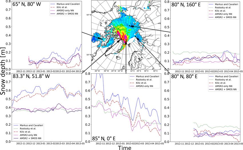
2432                  A. Braakmann-Folgmann and C. Donlon: Estimating snow depth on sea ice with a neural network

Figure 8. Time series of snow depth over one winter season 2012/2013 at different locations in the Arctic. The different algorithms are
represented by different colours and lines. Snow depth on FYI in lower latitudes is only recorded once SIC has reached 80 %.

depth vary depending on the algorithm. Most striking is, that         likely because of less snowfall, a densification of the snow in
in the middle of March the neural networks and the algorithm          winter and primarily ice drift from the (north) east replacing
of Markus and Cavalieri (1998) observe an increase in snow            older ice with younger ice and thinner snow. In general, all
depth, while the approach by Kilic et al. (2019) leads to a de-       algorithms more or less agree on the main trends on MYI,
crease. Unfortunately no in situ measurements are available           but snow depths by Markus and Cavalieri (1998) and Kilic
for comparison to verify the actual situation.                        et al. (2019) are higher than snow depths by Rostosky et al.
   The two plots on the right show snow depth evolution on            (2018) and our neural networks. Here again we recall that the
FYI at 80◦ N, 80◦ E in the Kara Sea (lower panel) and at              algorithm by Markus and Cavalieri (1998) is not reliable over
80◦ N, 160◦ E very close to the MYI or minimum ice extent             MYI and tends to largely overestimate snow depth larger than
edge of 2012 (upper panel). For all three FYI plots one might         50 cm.
expect that snow depth would start at zero, when the new ice             Even though no real validation is possible over the whole
has just formed. In reality most algorithms start at approxi-         Arctic or outside the OIB season, from the verification and
mately 0.10 m and snow depth estimation from Rostosky et              inter-comparison results we present, we can conclude that
al. (2018) starts at 0.20 m. This can be explained by the fact        our neural network results are similar in comparison to other
that we start calculating snow depth once SIC has reached             approaches. This indicates that, although only trained in a
80 % and SIC algorithms are known to underestimate SIC                limited area and with spring data, the neural networks may be
when thin sea ice is present: Ivanova et al. (2014) showed            applied for the whole Arctic and during a full winter season.
that in the case of 100 % SIC, the NASA Team algorithm
will only reach 80 % SIC at 0.20 m SIT, so snow depth is not          4.1.3   Uncertainty estimation
calculated before the ice has grown 20 cm thick.
   The plots on the bottom left at 83.3◦ N, 51.8◦ W just north        Finally we assess the uncertainty of our neural networks to
of Greenland and in the bottom centre at 85◦ N, 0◦ E show             enable usage of this snow product in models or for SIT calcu-
snow depth on MYI. The left one is an example for high                lation. The very complex and highly non-linear relationship
snow depth all year round, while the one at the centre ex-            between the input and snow depth output hinders a stringent
hibits a decrease in snow depth throughout winter. This is            variance propagation. Instead, to assess the uncertainty of

The Cryosphere, 13, 2421–2438, 2019                                                        www.the-cryosphere.net/13/2421/2019/
A. Braakmann-Folgmann and C. Donlon: Estimating snow depth on sea ice with a neural network                                   2433

our neural network approaches, we employ the Monte Carlo        Table 3. RMSE, correlation, coefficient of determination and bias
method and generate an ensemble of 50 samples for each in-      between CryoSat-derived SIT using different snow products and
put brightness temperature. We draw these samples from a        OIB-measured snow (italic) for all data. The best score of each cat-
normal distribution using the observed brightness tempera-      egory is highlighted in bold.
ture as mean and 0.5 K as standard deviation for AMSR2.
   For SMOS we take the standard deviation provided in the                                      RMSE       CC      R2        Bias
L3 files for each observation and propagate them through         Warren climatology (1999)      0.73 m    0.75   0.49      0.25 m
our averaging process to obtain a standard deviation for each    Modified Warren                0.67 m    0.77   0.57      0.16 m
SMOS measurement used as input to the polarization ratio.        Markus and Cavalieri (1998)    0.76 m    0.79   0.46      0.39 m
The mean of these standard deviations is 0.76 K for V po-        Rostosky et al. (2018)         0.65 m    0.79   0.62      0.08 m
                                                                 Kilic et al. (2019)            0.63 m    0.81   0.62      0.13 m
larization and 0.79 K for H polarization. Further uncertainty
                                                                 OIB snow                       0.62 m    0.80   0.63     –0.04 m
arises from the tie points used both in the NASA Team al-
gorithm for SIC and to correct the open-water part of the        AMSR2-only NN                  0.62 m    0.80   0.63    −0.05 m
footprint (Eq. 2). Therefore we also create an ensemble of 50    AMSR2 + SMOS NN                0.63 m    0.79   0.63    −0.06 m
samples for each tie point using the values from Ivanova et
al. (2014) as mean and 3 K as standard deviation. The result-
ing mean uncertainty in SIC from the NASA Team algorithm
is 4 %.
   We then estimate snow depth using each ensemble mem-
ber as input to our neural networks. This yields an ensem-
ble of snow depth estimates. The standard deviation of this
ensemble is used as an uncertainty measure for the esti-
mated snow depth value. Across all OIB data the resulting
final uncertainty (mean standard deviation) is 0.05 m for the
AMSR2-only NN and 0.02 m for the AMSR2 + SMOS NN,
indicating that the AMSR2 + SMOS NN is less sensitive
to noise in the input data. The error (repeatability) of the
Monte Carlo simulation is 0.0005 and 0.0001 m respectively.
This approach however only assesses how robust the neural
networks are to uncertainty in the input data and auxiliary
parameters such as the tie points. Further uncertainty arises
from training the neural networks with OIB data, which have
their own uncertainty and limitations unlike a real ground
truth dataset.

4.2   Results on sea ice thickness
                                                                Figure 9. OIB-measured SIT (all data) versus estimated SIT using
Having assessed the different snow depth algorithms, we now     CryoSat freeboard with different snow depth algorithms.
investigate how they influence SIT retrieval from CryoSat
freeboard data and compare the results to OIB-measured SIT.
In addition to the algorithms discussed above, we also in-      worse, which is not significant considering that the accuracy
clude the original (Warren et al., 1999) and modified (i.e.     of the OIB SIT is at best 5 cm. Therefore the last digit of
halved over FYI; Kurtz and Farrell, 2011) Warren climatol-      the bias and the RMSE should not be overrated. Concerning
ogy and the OIB-measured snow depth, which was used as          the correlation coefficient, using snow depth from Kilic et al.
validation snow depth data before. The results are presented    (2019) gives the best result, but the difference to other algo-
in Table 3 and visualized in Fig. 9.                            rithms is marginal. For the coefficient of determination, both
   Using the OIB-measured snow depth yields the lowest          our neural networks are as good as the OIB snow product
bias and RMSE, the highest coefficient of determination, and    closely followed by the algorithms by Rostosky et al. (2018)
the second highest correlation coefficient. Therefore using     and Kilic et al. (2019). Also in terms of bias, our neural net-
it as validation data for snow depth seems justified. How-      works show the second highest agreement with the OIB SIT,
ever, the difference in the snow depth algorithms is not that   just after the OIB-measured snow depth. For the Warren cli-
large, when they are used in SIT retrieval. In terms of RMSE    matology we observe that the modified version performs bet-
our AMSR2-only neural network performs as good as the           ter in all the categories, but still worse than most other algo-
OIB snow product and both the algorithm by Rostosky et al.      rithms. The approach of Markus and Cavalieri (1998) may
(2018) and the AMSR2+SMOS neural network are only 1 cm          perform equally well on FYI. Here we include the perfor-

www.the-cryosphere.net/13/2421/2019/                                                   The Cryosphere, 13, 2421–2438, 2019
You can also read