Marked decrease in the near-surface snow density retrieved by AMSR-E satellite at Dome C, Antarctica, between 2002 and 2011
←
→
Page content transcription
If your browser does not render page correctly, please read the page content below
The Cryosphere, 13, 1215–1232, 2019
https://doi.org/10.5194/tc-13-1215-2019
© Author(s) 2019. This work is distributed under
the Creative Commons Attribution 4.0 License.

Marked decrease in the near-surface snow density retrieved
by AMSR-E satellite at Dome C, Antarctica,
between 2002 and 2011
Nicolas Champollion1,a , Ghislain Picard1 , Laurent Arnaud1 , Éric Lefebvre1 , Giovanni Macelloni2 , Frédérique Rémy3 ,
and Michel Fily1
1 Institut des Géosciences de l’Environnement (UMR 5001), CNRS/UGA/Grenoble-INP/IRD,
CS 40700, 38058 Grenoble CEDEX 9, France
2 Institute of Applied Physics, IFAC/CNR, Via Madonna del Piano 10, 50019 Fiorentino, Italy
3 Laboratoire d’Étude en Géophysique et Océanographie Spatiales (UMR 5566), UPS/CNRS, 18 av. Edouard Belin,

31401 Toulouse CEDEX 9, France
a now at: The Climate Lab, University of Bremen, Celsiusstrasse 2 FVG–M2040, 28359 Bremen, Germany

Correspondence: Champollion Nicolas (nicolas.champollion@uni-bremen.de)

Received: 30 November 2018 – Discussion started: 7 December 2018
Revised: 11 March 2019 – Accepted: 17 March 2019 – Published: 12 April 2019

Abstract. Surface snow density is an important variable for      satellites, though the link to the density is more difficult to
the surface mass balance and energy budget. It evolves ac-       establish. However, no related pluri-annual change in mete-
cording to meteorological conditions, in particular, snowfall,   orological conditions has been found to explain such a trend
wind, and temperature, but the physical processes govern-        in snow density. Further work will concern the extension of
ing atmospheric influence on snow are not fully understood.      the method to the continental scale.
A reason is that no systematic observation is available on a
continental scale. Here, we use the passive microwave obser-
vations from AMSR-E satellite to retrieve the surface snow       1   Introduction
density at Dome C on the East Antarctic Plateau. The re-
trieval method is based on the difference of surface reflec-     Snow density is an important variable that relates snow thick-
tions between horizontally and vertically polarized bright-      ness and mass. Close to the surface, knowledge of its value
ness temperatures at 37 GHz, highlighted by the computa-         is necessary to establish the surface mass balance from in
tion of the polarization ratio, which is related to surface      situ measurements using stakes, ultrasonic sensors, ground-
snow density. The relationship has been obtained with a mi-      penetrating radar, snow pits or firn cores (Eisen et al., 2008),
crowave emission radiative transfer model (DMRT-ML). The         and satellite observations (microwave radiometer and lidar
retrieved density, approximately representative of the top-      or radar altimeters, Arthern et al., 2006; Flament and Rémy,
most 3 cm of the snowpack, compares well with in situ mea-       2012; McMillan et al., 2014; Palerme et al., 2014; Markus
surements. The difference between mean in situ measure-          et al., 2017). It is useful for the validation of regional cli-
ments and mean retrieved density is 26.2 kg m−3 , which is       mate modelling (Lenaerts and van den Broeke, 2012; Fet-
within typical in situ measurement uncertainties. We apply       tweis et al., 2013; Vernon et al., 2013). Surface snow density
the retrieval method to derive the time series over the pe-      is also important to the study of the surface energy budget
riod 2002–2011. The results show a marked and persistent         (Brun et al., 2011; Favier et al., 2011; Libois et al., 2013;
pluri-annual decrease of about 10 kg m−3 yr−1 , in addition to   Fréville et al., 2014), firn densification (Alley et al., 1982;
atmosphere-related seasonal, weekly, and daily density vari-     Fujita et al., 2011), and air–snow exchanges (Domine et al.,
ations. This trend is confirmed by independent active mi-        2008; France et al., 2011). Its evolution is related to the lo-
crowave observations from the ENVISAT and QuikSCAT               cal meteorological conditions, such as precipitation, wind

Published by Copernicus Publications on behalf of the European Geosciences Union.
1216                                        N. Champollion et al.: Decrease in the snow density near the surface at Dome C

speed, and air temperature (Brun et al., 2011; Champollion          ferent layers of the snowpack. The electromagnetic reflec-
et al., 2013; Libois et al., 2014; Fréville et al., 2014). How-     tions at each interface between layers with different densities
ever, their links are complex and not well known. For exam-         (air–snow or internal snow–snow interfaces) are calculated
ple, snowfall can lead to different surface density behaviours      with Fresnel equations that use the snow permittivity and de-
depending on initial snow conditions: over hard and dense           pend on the polarization (Born and Wolf, 1999). As a conse-
surface snow, snowfall results in a decrease in surface snow        quence, snow density greatly influences the polarization of
density; over surface hoar crystals, snowfall increases surface     microwave radiation, which was noted in previous studies
snow density. The interactions between the different meteo-         (Shuman et al., 1993; Shuman and Alley, 1993; Abdalati and
rological effects are more complex. Wind often increases sur-       Steffen, 1998; Liang et al., 2009; Champollion et al., 2013;
face snow density (Sommer et al., 2018), and water vapour           Brucker et al., 2014; Leduc-Leballeur et al., 2015, 2017).
fluxes into the snowpack are regularly oriented towards the         Using the Dense Media Radiative Transfer - Multi Layers
atmosphere, resulting in a decrease in the density near the         model (DMRT-ML, Tsang et al., 2000a; Roy et al., 2012; Pi-
surface. However, wind can also contribute to the sublima-          card et al., 2013; Dupont et al., 2013), we quantitatively de-
tion of snow and thus change snow metamorphism (Domine              termine the influence of surface snow density on microwave
et al., 2008).                                                      polarization ratio. This relationship is then used to retrieve
   Estimating the surface snow density in Antarctica remains        the density from satellite observations, which are measured
difficult (Eisen et al., 2008; Groot Zwaaftink et al., 2013). It    by the Advanced Microwave Scanning Radiometer – Earth
is presently not retrieved from satellite remote sensing (Groh      observing system (AMSR-E) instrument. In situ measure-
et al., 2014), and the snow density estimates from regional         ments of snow properties are used as input for the DMRT-
climate and snowpack modelling are highly uncertain close           ML model. Active microwave observations and in situ mea-
to the surface (Brun et al., 2011; Fettweis et al., 2013). Nev-     surements of surface snow density are used to validate the
ertheless, Schwank and Naderpour (2018) recently presented          method.
encouraging results about the retrieval of snow density from           Section 2 presents remote sensing and in situ data and
ground-based L-band radiometry. However, this method is             the microwave emission model. Section 3 presents some el-
valid only for a soil bottom layer. In addition, despite some       ements of the theoretical background of microwave radiative
recent progress towards automatically measuring the snow            transfer, and Sect. 4 presents the method of retrieving the sur-
density in the field (Mittal et al., 2009; Gergely et al., 2010),   face snow density. Section 5 presents the time series of the
manual measurements are more accurate, with a typical accu-         retrieved surface snow density and its validation and analy-
racy around 11 % (Conger and McClung, 2009). This results           sis.
in a low spatial and temporal coverage of Antarctica, espe-
cially on the East Antarctica Plateau where data are mainly
acquired during traverses or close to stations (Favier et al.,      2     Data and model
2013; Groot Zwaaftink et al., 2013). Close to the surface,
                                                                    Satellite remote sensing datasets, measurements of snow
the measurements are more difficult and uncertain due to
                                                                    properties, and the microwave radiative transfer model are
the surface irregularity, resulting in uncertainties higher than
                                                                    described in the three following sections.
11 % (Gallet et al., 2011, 2014; Champollion et al., 2013; Li-
bois et al., 2014). Finally, an intercomparison exercise has        2.1     Satellite observations
recently shown that snow densities measured by different
methods in the Swiss Alps agree within 9 % and that the ver-        2.1.1    Passive microwave data
tical density variations are not completely captured (Proksch
et al., 2016).                                                      Passive microwave satellite observations were acquired at
   The objective of this study is to develop and validate a         18.7 and 36.5 GHz by the AMSR-E instrument on-board the
new method of determining the snow density near the surface         Aqua satellite in dual-polarization mode with an observation
from passive microwave satellite observations. The study is         zenith angle of 54.8◦ over the entirety of the instrument’s
performed at Dome C (75◦ 060 S, 123◦ 210 E), on the East            lifetime, i.e. from 18 June 2002 to 4 October 2011. Daily av-
Antarctic Plateau, where the French–Italian base of Concor-         eraged brightness temperatures (TB ) at Dome C are extracted
dia is located, combining in situ data of snow properties and       from the “AMSR-E/Aqua Daily L3 25 km Brightness Tem-
electromagnetic modelling. Except for melting regions, the          perature & Sea Ice Concentration Polar Grids, Version 3”
method has the potential for a global spatial coverage of the       provided by the National Snow and Ice Data Center (NSIDC,
Antarctic Ice Sheet, which will be addressed in further work.       Cavalieri et al., 2014). The pixel size is 25 km × 25 km and
Following Brucker et al. (2011), we first simulate the snow         the total sensor error is around 0.6 K. The dataset contains,
microwave emission and thus quantify its sensitivity to snow        for every day, the mean of the daily averaged ascending or-
properties. Qualitatively, it is well known that the permittiv-     bits and daily averaged descending orbits. This typically rep-
ity of snow is highly dependent on density (Mätzler et al.,         resents seven overpasses per day at Dome C.
1984; Warren and Brandt, 2008) and thus changes in the dif-

The Cryosphere, 13, 1215–1232, 2019                                                      www.the-cryosphere.net/13/1215/2019/
N. Champollion et al.: Decrease in the snow density near the surface at Dome C                                               1217

   A detailed analysis of the spatial and temporal variabil-        2.2     In situ snow measurements
ity of passive microwave data close to Dome C is given by
Long and Drinkwater (2000), Macelloni et al. (2007), Picard         Snow observations include the snow density near the surface
et al. (2009), and Brucker et al. (2011). As in these previ-        and the vertical profiles of snow temperature, density, and
ous studies, we assume that (1) only one or a few in situ           specific surface area (SSA).
measurements are sufficient to model the brightness temper-
ature of an entire satellite pixel and (2) the pixel containing     2.2.1    Surface snow density
in situ measurements is representative of the satellite pixels
around Dome C. These assumptions have been validated us-            Three time series of snow density were measured at Dome C.
ing ground-based radiometers by Picard et al. (2014), who           The first set of measurements is from the CALVA programme
found that the Dome C area was sufficiently homogeneous.            (CALibration-VAlidation of climate models and satellite re-
                                                                    trieval, Antarctic coast to Dome C). Surface snow density
2.1.2   Active microwave data                                       was measured every 3 to 5 days from 3 February 2010 to
                                                                    4 October 2011 by using a cylinder cutter (10 cm length
Two complementary datasets of active microwave observa-             and diameter of 5 cm) inserted horizontally so that the cut-
tions are used for comparison with the retrieved snow den-          ter top grazes the surface. The value used here is the aver-
sity. The first dataset was acquired by the nadir-looking           age of three measurements. The two other sets of measure-
Radar Altimeter 2 (RA-2) instrument on-board the ENVI-              ments are from the project MAPME (Monitoring of Antarctic
ronment SATellite (ENVISAT) at 13.6 GHz (Ku band). The              Plateau by means of Multi-Frequency Microwave Emission)
dataset contains the total backscatter power from 12 March          funded by PNRA (Programma Nazionale di Ricerche in An-
2002 to 8 April 2012 based on along-track data and the Ice-         tartide). The second dataset contains the snow density mea-
2 retracking algorithm (Legrésy et al., 2005; Rémy et al.,          sured from 9 May 2008 to 4 October 2011 by using a cylin-
2014). Radar backscatter corresponds to the ratio between           der cutter of 25 cm height and a diameter of 4.5 cm. Measure-
the energy emitted by the satellite and the energy reflected        ments were performed at 0.1 m depth every 15 days in a snow
by the snow surface and is expressed in decibels. Due to the        stake network composed of eight poles placed 10 m apart .
35 days of ENVISAT revisit time and the selection of four           The value used here is the average of eight measurements.
orbit tracks that are less than 17 km away from Concordia           The last dataset contains the snow density measured in snow
station, temporal sampling of RA-2 observations is typically        pits, which were excavated every month from 18 Decem-
8–10 days. The along-track spatial sampling over the Antarc-        ber 2007 to 4 October 2011. Density values were collected
tic Ice Sheet is 330 m, and its typical footprint is of the order   every 10 cm in the 0–1 m depth range. A single measurement
of 5–10 km (Rémy and Parouty, 2009). The sensor precision           was collected at each depth of the snow pit.
for determining surface elevation is 47 cm.                            The mean density value is 329, 344, and 321 kg m−3 ,
   The second dataset of active microwave observations              respectively, for the CALVA dataset and the two PNRA
was acquired by the SeaWinds instrument on-board the                datasets. The standard deviation is, respectively, 43, 40, and
Quick SCATterometer (QuikSCAT) at 13.4 GHz in dual-                 54 kg m−3 . The density is representative of the topmost 5 cm
polarization mode. Zenith viewing angles are 46 and 54.1◦           of the snowpack for the CALVA dataset and of the top 10 cm
for horizontal and vertical polarizations, respectively. Nor-       for the two PNRA datasets. Uncertainties associated with the
malized radar cross sections σ 0 were extracted at Dome C           three datasets are equal to or higher (due to the low cohesion
from the “egg images of SeaWinds on QuikSCAT Enhanced               of surface snow) than the uncertainty estimated for classic
Spatial Resolution Image Sigma-0 Products – version 2” pro-         density measurements (11 %, Conger and McClung, 2009).
vided by the National Aeronautics and Space Administra-                For the first time, the spatial variability of surface snow
tion – Scatterometer Climate Record Pathfinder (http://www.         density measurements has been assessed with three series
scp.byu.edu/data/Quikscat/SIRv2/Quikscat_sirV2.html, last           of 40 measurements (measurements taken every 1, 10, and
access: 8 April 2019, Long and Daum, 1998; Early                    100 m). The averages and standard deviations are, respec-
and Long, 2001; Long et al., 2001). The pixel size                  tively, 298.7 ± 29.3, 317.6 ± 24.7, and 307.9 ± 59.8 kg m−3
is 2.225 km × 2.225 km and the relative error is 0.2 dB             for metre, decametre, and hectometre scales. Considering all
(Spencer et al., 2000; Early and Long, 2001). The dataset           measurements (n = 120), we found a mean density and stan-
contains the daily averaged backscatter coefficient by com-         dard deviation of 308.3 ± 41.6 kg m−3 . Under the assump-
bining multiple passes of QuikSCAT (near-polar orbit) from          tion of a normal distribution of snow density measurements,
19 July 1999 to 23 November 2009.                                   the value 83.2 kg m−3 covers 95 % of the distribution vari-
                                                                    ance. This value represents 26.9 % of the mean density and
                                                                    is assumed to represent the spatial variability of surface snow
                                                                    density measurements around Dome C. We also assume that
                                                                    there were no changes in the spatial variability during the
                                                                    study period (2002–2011).

www.the-cryosphere.net/13/1215/2019/                                                     The Cryosphere, 13, 1215–1232, 2019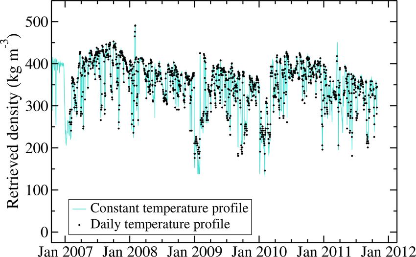
1218                                         N. Champollion et al.: Decrease in the snow density near the surface at Dome C

                                                                     2.2.3   Snow density profile

                                                                     The snow density profile (Fig. 1) is considered constant and
                                                                     is composed of two different datasets. The first dataset was
                                                                     measured in January 2010 by determining the mass and vol-
                                                                     ume of snow and firn core samples every 5 cm, collected
                                                                     up to 20 m depth. However, the cohesion of the first 0.3 m
                                                                     of the snow core was very low and impossible to sample
                                                                     correctly. Thus, a second dataset was measured in Decem-
                                                                     ber 2010 to complete the snow density profile from the sur-
                                                                     face down to 0.3 m depth. This second dataset is an average
                                                                     of 13 short density profiles (up to 0.5 m depth) measured in
                                                                     a snow pit with a dedicated cutter for Antarctic snow (Gallet
                                                                     et al., 2011).
                                                                        The snow core and snow pit density profiles below
Figure 1. The measured profiles of snow density, SSA, and DMRT-
                                                                     0.3 m depth are close together. Indeed, the mean and
ML radius at Dome C, Antarctica. DMRT-ML radius is derived
from SSA measurements and is the input of the model (Sect. 2.2.4
                                                                     standard deviation of both profiles (0–0.5 m deep) are
and Eqs. 1 and 2).                                                   about 340 ± 8 kg m−3 for the snow core dataset and about
                                                                     355 ± 21 kg m−3 for the snow pit dataset. In addition, the
                                                                     overlapping part (between 0.3 and 0.5 m depth) shows sim-
2.2.2   Snow temperature profile                                     ilar values. Uncertainties associated with both methods are
                                                                     similar: at least 10 % for measurements of snow and firn core
Snow temperature was recorded every hour from 1 Decem-               samples (Arthern et al., 2010) and at least 11 % for snow
ber 2006 to 4 October 2011 and from the surface to 21 m              cutter measurements in a snow pit (Conger and McClung,
depth, with 35 probes initially installed every 0.1 m down           2009).
to 0.6 m depth, every 0.2 m down to 2 m, every 0.5 m down
to 5 m, and every 1 m down to 21 m. The probes are lo-               2.2.4   Snow-specific surface area profile
cated around 1 km west of the Concordia station. All probes
(100  platinum resistance sensors with an accuracy better           The snow SSA (Fig. 1) is the surface area of ice crystals
than ±0.1 K at 223 K) were inter-calibrated with a precision         divided by the mass of snow (Domine et al., 2006; Arnaud
of ±0.02 K. The probes are continuously being buried over            et al., 2011). Its profile up to 20 m depth was measured in
time due to snow accumulation, which is estimated to be              January and December 2010 using the Profiler Of Snow-
around 0.1 m yr−1 (Frezzotti et al., 2005, 2013; Arthern et al.,     Specific Surface area Using short-wave infrared reflectance
2006; Eisen et al., 2008; Brucker et al., 2011; Verfaillie et al.,   Measurement instrument (POSSSUM, Arnaud et al., 2011)
2012). Initial probe depths are corrected as a function of the       and the Alpine Snow Specific Surface Area Profiler (ASS-
date measurements. In addition, the temperature measure-             SAP, Champollion, 2013; Libois et al., 2014), which is a
ments closest to the surface become deeper and deeper over           lightweight version of POSSSUM adapted for shallow snow-
time. This means that no measurements are taken in the upper         packs (maximum 2 m deep). These two instruments are based
snowpack. To correct for this issue, we extrapolate the pro-         on the relationship between snow reflectance in the near-
files using an exponential function between the uppermost            infrared domain and snow SSA (Domine et al., 2006; Matzl
probe in the snowpack and the temperature at the surface (Pi-        and Schneebeli, 2006). Using a laser at 1310 nm illuminat-
card et al., 2009; Brucker et al., 2011; Groot Zwaaftink et al.,     ing the face of a snow hole and a specific data processing
2013). The latter is approximated by the 2 m air temperature.        algorithm (Arnaud et al., 2011), POSSSUM and ASSSAP
Air temperature was extracted from the global ERA-Interim            instruments determine the snow SSA as a function of depth
reanalysis provided by the European Centre for Medium-               in the field. Uncertainty associated with SSA measurements
range Weather Forecasts (ECMWF, Dee et al., 2011), which             from POSSSUM is about 10 % (Arnaud et al., 2011). Both
is considered the superior reanalysis in the East Antarctica         instruments are very similar and have been compared multi-
region (Xiie et al., 2014). We use passive microwave obser-          ple times, thereby ASSSAP uncertainty is considered to be
vations that are daily, which is why we calculate daily av-          10 % as well.
eraged temperature by averaging two hourly profiles (14:00              Larger errors were found above 0.3 m depth using POSS-
and 00:00 LT).                                                       SUM than when using ASSSAP. Thus, we decided to use
                                                                     SSA measurements from ASSSAP for the first 0.3 m and
                                                                     POSSSUM observations below. SSA profiles from both in-
                                                                     struments overlap between 0.3 and 0.5 m depth and show
                                                                     very close values. Averaged SSA values from ASSSAP are

The Cryosphere, 13, 1215–1232, 2019                                                     www.the-cryosphere.net/13/1215/2019/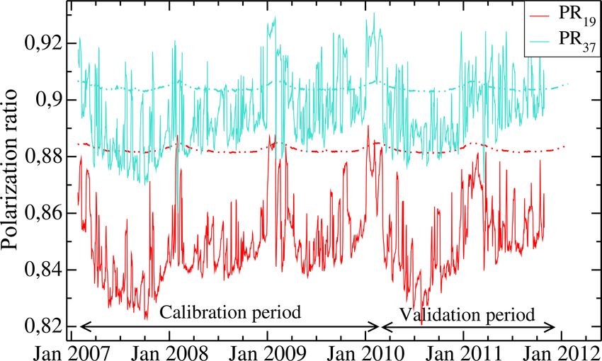
N. Champollion et al.: Decrease in the snow density near the surface at Dome C                                                   1219

13.2 and 13.9 m2 kg−1 for POSSSUM. Due to an artefact                 In addition, two criteria must be respected in the framework
that increases the measured SSA when the hole is drilled              of DMRT theory: snow density less than 300–350 kg m−3
for snow below 5 m (Picard et al., 2014), we removed the              (Liang et al., 2006; Tsang et al., 2008) and low optical ra-
measured values and replaced them with a constant value               dius with respect to the wavelength (Rayleigh scattering).
(SSA5 m ). This value is optimized following Brucker et al.           The latter is always respected in our study since rDMRT-ML
(2011) (Sect. 5.1).                                                   never exceeds 0.6 wavelengths and most of the time is lower
   The snow SSA is not directly used in DMRT-ML model.                than 0.1. Regarding when the density is sometimes higher
The snow parameter that characterizes the snow grain size             than 350 kg m−3 in our profile (Fig. 1), Picard et al. (2013)
in the electromagnetic model (rDMRT-ML , Fig. 1) is related           explained that the deviation in scattering and absorption co-
to the optical radius (ropt ). The relationships between snow         efficients remains moderate.
SSA, DMRT-ML radius, and optical radius are given by the
following equations:                                                  2.3.2    Atmospheric contribution

rDMRT-ML = φ · ropt ,                                          (1)    The atmosphere attenuates the microwave emissions emerg-
SSA = (3 · φ)/(ρice · ropt ),                                  (2)    ing from the surface and itself emits microwaves due to its
                                                                      own temperature (Rosenkranz, 1992). Although this effect
where φ is a snow microstructure parameter that depends on            is low over the Antarctica Plateau because of the low atmo-
the shape of snow crystals and the stickiness and size dis-           spheric humidity and the small size of scatterers in the atmo-
tribution of ice crystals (Brucker et al., 2011; Roy et al.,          sphere (Walden et al., 2003; Genthon et al., 2010), both ef-
2012; Dupont et al., 2013) and ρice is the density of ice, i.e.       fects are taken into account in our modelling on a daily basis
917 kg m−3 . The φ parameter is optimized as in Brucker et al.        with a simple non-scattering radiative transfer scheme. Top-
(2011) (Sect. 5.1).                                                   of-atmosphere (TOA) brightness temperatures are computed
                                                                      using the method and equations from Rosenkranz (1992)
2.3     Microwave emission model                                      and following Picard et al. (2009). Upward and downward
                                                                      atmospheric TB ’s are calculated using atmospheric temper-
2.3.1    Snow microwave emission
                                                                      ature and moisture profiles from ERA-Interim reanalysis.
The snow microwave emission model DMRT-ML (Picard                     The transmission coefficient is 0.960 at 37 GHz and 0.987
et al., 2013) has already been applied and validated in sev-          at 19 GHz, and the downward cosmic TOA TB is 2.75 K.
eral studies (Brucker et al., 2011; Roy et al., 2012; Dupont
et al., 2013; Picard et al., 2014) and is freely available (http://   3     Theoretical background in microwave remote
pp.ige-grenoble.fr/pageperso/picardgh/dmrtml/, last access:                 sensing
8 April 2019). It allows the computation of the top-of-
snowpack emerging brightness temperature for a given snow-            Some elements of the theoretical background of microwave
pack at different viewing angles, at different frequencies, and       satellite remote sensing are described in the next two sec-
at both vertical and horizontal polarizations. The model is           tions.
composed of two parts: (1) the DMRT theory to calculate the
absorption and scattering coefficients for all snow layers – in       3.1     Passive microwave remote sensing
the model, the snowpack is composed of horizontally semi-
infinite and vertically homogeneous snow layers of dense              We use the brightness temperature polarization ratio (PR)
ice spheres, completely defined by the layer thickness, tem-          at 19 and 37 GHz to increase the sensitivity of passive mi-
perature, density, and optical radius of snow – and (2) the           crowave observations to surface properties (Shuman et al.,
DIScrete Ordinate Radiative Transfer method (DISORT, Jin,             1993; Surdyk, 2002a; Champollion et al., 2013):
1994) to propagate the thermal emission of each snow layer                     TB (ν, h)
from the bottom of the snowpack to the atmosphere. DIS-               PRν =              ,                                         (3)
                                                                               TB (ν, v)
ORT accounts for multiple scattering between layers. Layers
are assumed to be planes, parallel, and much thicker than the         where TB (ν, α) is the brightness temperature, ν the fre-
wavelength.                                                           quency, and α the polarization.
   We use the model in a non-sticky grain configuration, i.e.            Champollion et al. (2013) showed that PR, at the AMSR-
grains which do not form aggregates, and with a unique opti-          E incidence angle, which is close to the Brewster angle for
cal radius of snow grains, i.e. no grain size distribution. Snow      the air–snow interface, mainly depends on the snow density
crystal aggregates are not considered in this study because           near the surface, the surface roughness, and the vertical snow
the φ parameter used to convert snow SSA into an optical              stratification, i.e. abrupt changes in the snow density pro-
radius partly integrates this snow property (Roy et al., 2012;        file. We consider flat interfaces that neglect the influence that
Löwe and Picard, 2015). We also use a semi-infinite bottom            roughness has on PR (the relevance of this assumption is ex-
snow layer to consider the firn of the Antarctic Ice Sheet.           plained in Sect. 5.5). Consequently, the polarization ratio is

www.the-cryosphere.net/13/1215/2019/                                                         The Cryosphere, 13, 1215–1232, 2019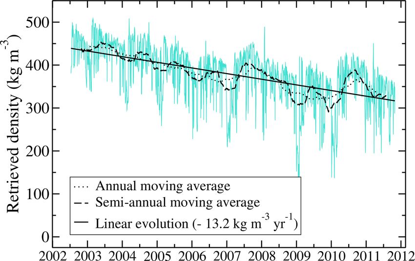
1220                                       N. Champollion et al.: Decrease in the snow density near the surface at Dome C

a non-linear combination of surface and internal reflections       4    Method
(Leduc-Leballeur et al., 2017).
   In order to understand the polarization ratio evolution, two    The different steps of the method of retrieving the surface
cases are explored: (1) snow properties that vary with depth       snow density are described in this section. Surface density
but are constant in time and (2) snow properties that also         variations are deduced from the PR evolution. However, to
vary over time. For case (1), the PR evolution is only due to      correctly simulate PR evolution, we first need to simulate the
changes in the snow density near the surface. For case (2), PR     mean state of the PRs.
evolution is also influenced by changes in the snow density
stratification. Snow evolution is mainly influenced by atmo-           1. In the first step, we follow the forward modelling ap-
spheric conditions. The surface is first affected and then at-            proach of Brucker et al. (2011) to simulate the time se-
mospheric influence diffuses deeper into the snowpack. This               ries of brightness temperatures, using the vertical pro-
process is slow on the Antarctica Plateau (Surdyk, 2002b;                 files of snow properties, which, except for the temper-
Brucker et al., 2011; Picard et al., 2014; Libois et al., 2014)           ature, are kept constant over time. From the simulated
and implies a slower evolution of snow deeper into the snow-              brightness temperatures, we calculate the time series of
pack than near the surface. As a result, the PR evolution is              polarization ratios and show the correct simulation of
primarily influenced by surface snow density variations (the              the mean polarization ratios and the poor modelling of
relevance of this assumption is explained in Sect. 5.5).                  their temporal variations.

3.2    Active microwave remote sensing
                                                                       2. In the second step, we simulate the polarization ratio
The signal returned by the snowpack is a complex combi-                   variations due to changes in the properties of a 0.03 m
nation of surface and volume scattering (Rémy and Parouty,                snow layer on top of the snowpack theoretically (as in
2009; Rémy et al., 2014; Tedesco, 2015; Adodo et al., 2018).              Leduc-Leballeur et al., 2015, 2017), and we also show
The surface-to-subsurface signal ratio is used to determine               the strong relationship between PR at 37 GHz and the
the main contributor to radar backscatter observations. On                density of this surface layer.
the East Antarctica Plateau this ratio is high (Lacroix et al.,
2008, 2009), and thus surface echo is the main contributor             3. The third step corresponds to the retrieval algorithm it-
to the radar backscatter at Dome C. Consequently, the long-               self. We estimate the time series of surface snow density
term evolution of ENVISAT observations mainly depends on                  by minimizing the deviations between the modelled and
surface snow density and roughness.                                       observed polarization ratio at 37 GHz.
   Because the incidence angles of the SeaWinds instrument
are close to the Brewster angle for the air–snow interface,           Some studies have reported high vertical snow stratifica-
the surface reflection at vertical polarization is weakly influ-   tion around Dome C (Gallet et al., 2014; Picard et al., 2014).
enced by the near-surface snow density. Consequently, the          They observed very dense and thick snow layers (about
evolution of the radar backscatter coefficient at vertical po-     500 kg m−3 for 0.3–0.5 m thick), and thin and low-density
larization is mostly dependent on surface roughness changes.       layers (less than 150 kg m−3 for a thickness of few cen-
Therefore, considering the independence of volume scatter-         timetres). The poor modelling of the horizontally polarized
ing from the polarization (Tsang et al., 2000b; Picard et al.,     brightness temperature could be due to an underestimation
2013), as well as the independence of surface roughness ef-        of the snow stratification (Macelloni et al., 2007; Brucker
fect from the polarization (Ulaby et al., 1982; Adodo et al.,      et al., 2011; Champollion et al., 2013; Picard et al., 2013;
2018), we defined the radar polarization ratio (RPR) to be         Leduc-Leballeur et al., 2015). In order to correctly simulate
primarily influenced by the snow density near the surface          the mean horizontally polarized brightness temperatures, and
(Liang et al., 2008):                                              thus the mean polarization ratios, we added, at 0.1 and 0.2 m
                                                                   depth in our snow density profile, two layers that were 0.1
                0
         σh0   rh, surface                                         and 0.2 m thick with a density equal, respectively, to 225 and
RPR =        '             ,                                (4)    500 kg m−3 .
         σv0    0
               rv, surface

where σ 0 is the radar backscatter coefficient, r 0 is the part
of backscatter coefficient considering only the surface reflec-    5    Results and discussion
tion, and h and v are the polarizations. For simplicity, the ν
index is not written.                                              The results of the different steps to retrieve the surface snow
                                                                   density are presented in the next three sections. The fourth
                                                                   section is dedicated to the comparison and validation of the
                                                                   retrieved density, and the last section examines the different
                                                                   sources of uncertainties.

The Cryosphere, 13, 1215–1232, 2019                                                      www.the-cryosphere.net/13/1215/2019/
N. Champollion et al.: Decrease in the snow density near the surface at Dome C 1221
Figure 3. Time series of modelled (lines) and observed (dots) po-
larization ratios at 19 and 37 GHz (PR19 and PR37 ) at Dome C,
Antarctica, during the calibration period (2007–2009) and the vali-
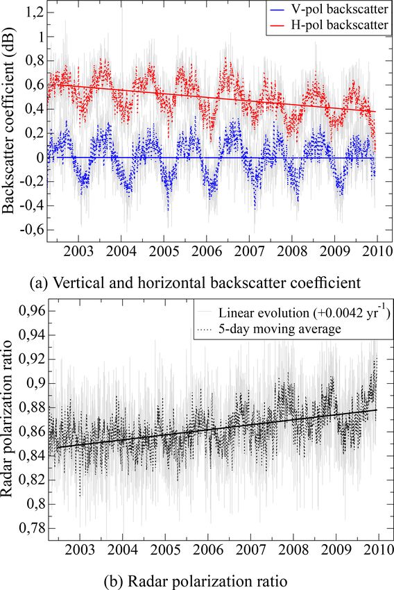
Figure 2. Time series of modelled (lines) and observed (dots) dation period (2010–2011).
brightness temperatures, at 19 and 37 GHz and at vertical and hori-
zontal polarizations – TB (19, V), TB (19, H), TB (37, V) TB (37, H) –
at Dome C, Antarctica, during the calibration period (2007–2009)
and the validation period (2010–2011). 2.5, which is in the range of those found by Brucker et al.
(2011) and Picard et al. (2014), respectively, 2.8 and 2.3, with
an RMSE of 1.6 K. Observed brightness temperatures are
5.1 Time series simulation well reproduced by the DMRT-ML model both in terms of
absolute value and evolution, except for 19 GHz at horizontal
TOA horizontally and vertically polarized brightness tem-
polarization. The RMSE calculated by excluding TB (19, H)
peratures at 19 and 37 GHz – written TB (19, V), TB (19, H),
is indeed 2.6 K, whereas RMSE 19, h is 7.4 K. Table 1 sum-
TB (37, V) and TB (37, H) – are simulated with the DMRT-ML
marizes all errors between observed and modelled TB ’s. The
model during the 3 years (from 1 December 2006 to 31 De-
RMSE during the calibration and validation periods are very
cember 2009) when the temperature profiles were recorded.
close, showing the high performance of the optimization. We
The two parameters SSA5 m and φ are optimized during this
also found a slight improvement in the modelled TB (19, H)
period of calibration by minimizing the root-mean-square er-
compared to Brucker et al. (2011) with an RMSE 19, h of
ror (RMSE) between the modelled and observed TB (19, V)
7.4 K instead of 8–10 K. These results confirm the represen-
and TB (37, V). As in Brucker et al. (2011), only the vertical
tativeness of the in situ measurements for the satellite pixel
polarization is used because of its high sensitivity to snow
encompassing Dome C (25 km × 25 km).
SSA and reduced sensitivity to density changes. TOA bright-
The polarization ratio evolution, calculated from the sim-
ness temperatures are then simulated over nearly 2 years of
ulated brightness temperatures, does not reproduce the ob-
validation (from 1 January 2010 to 4 October 2011) using the
served variations, and the 5-year average of modelled PR19
optimized SSA5 m and φ parameters. RMSEs are defined by
overestimates the observations by 0.033 (Fig. 3). This rep-
the following equations:
resents around 46 % of the maximum amplitude of observed
v
u n
PR19 variations. On the other hand, mean PR37 is well mod-
u1 X 2
RMSEν,α = t · obs
TB,i mod
(ν, α) − TB,i (ν, α) , (5) elled. The simulated mean PR37 is indeed 0.904, whereas the
n i=1 observed mean PR37 is 0.896. The difference represents only
q 11 % of the maximum amplitude of observed PR37 varia-
RMSEν = 0.5(RMSE2ν,v + RMSE2ν,h ), (6) tions. Table 2 summarizes all errors between observed and
s modelled PRs.
1 X
RMSE = · RMSE2ν,α , (7) The poor simulation of the mean PR19 comes from an in-
p ν,α correct simulation of TB (19, H) which, as explained in Arth-
ern et al. (2006), is mainly due to the stratification of the
where n is the number of observations, TB,i obs (ν, α) and
snowpack. Because PR37 is well reproduced, and considering
mod
TB,i (ν, α) the observed and modelled brightness tempera- that penetration depth is, respectively, around 5 and 1 m for
tures at ν frequency α polarization, and p = 4 the number of 19 and 37 GHz (Surdyk, 2002b), the stratification in the first
polarizations and frequencies used. metre of the snowpack is adequately represented. Hence, the
The time series of observed and modelled brightness tem- discrepancy between observed and modelled PR19 is prob-
peratures are shown in Fig. 2. The optimized SSA5 m and φ ably because of a stratification that is too weak below 1 m
parameters are, respectively, equal to 10.1 m2 kg−1 and to depth, and further works can address this issue by increasing
www.the-cryosphere.net/13/1215/2019/ The Cryosphere, 13, 1215–1232, 20191222 N. Champollion et al.: Decrease in the snow density near the surface at Dome C
Table 1. Errors between modelled and observed brightness temperatures (K) for the calibration and validation periods.
RMSE19, v RMSE19, h RMSE37, v RMSE37, h
Calibration period 0.63 7.6 2.1 3.7
Validation period 1.6 7.2 3.6 4.1
RMSEv RMSEh RMSE
Calibration period 1.6 6.0 4.4
Validation period 2.8 5.9 4.6
Table 2. Errors between modelled and observed polarization ratios 0.88 and 0.92. Moreover, this simulation shows the weak
for the calibration and validation periods. influence of the temperature profile on polarization ratio.
The larger variation due to the different temperature pro-
RMSEPR, 19 RMSEPR, 37 RMSE files is 0.0043, which represents only 7.25 % of the larger
Calibration period 0.039 0.017 0.030 PR variation caused by surface density changes (from 150
Validation period 0.031 0.011 0.023 to 450 kg m−3 ). This sensitivity analysis demonstrates the
strong relationship between the polarization ratio at 37 GHz
and surface snow density and thus shows the possibility of re-
trieving the density ρsat from the PR37 satellite observations.
the stratification deeper into the snowpack. The poor simula-
tion of the mean PR19 is not a major issue in this work since 5.3 Surface snow density evolution
we study the time variations in polarization ratios. However,
we decided to exclude 19 GHz data frequency in the follow- Surface snow density ρsat is estimated every day by mini-
ing in order to avoid introducing bias in the retrieved density. mizing the RMSE between the observed and modelled PR37
In contrast to the long-term average, the seasonal and and only changing the snow density of the top layer. The
faster variations in the polarization ratio at 37 GHz are not RMSE minimization is done though a Newton approach
reproduced. We explain this by the fact that the evolution (scipy.optimize.newton function of Python). This method en-
of polarization ratio is mainly governed by variations in the sures a quick convergence (typically after 3–5 iterations)
snow density close to the surface, whereas we have consid- with a residual RMSE less than 0.001. That translates into
ered the snow density profile constant over time in our simu- a precision of surface snow density equal to 3.5 kg m−3 . We
lation here. use a constant vertical profile of temperature equal to the 5-
year average of the vertical temperature profile measured in
5.2 Sensitivity analyses the field. This choice is motivated by the fact that no temper-
ature data are available before December 2006. However, the
In order to represent the snow evolution close to the surface results are weakly affected by this assumption (Sect. 5.5).
and thus to simulate PR37 variations, a thin layer (0.03 m Because of the 5-year average, the temperature profile is
thick) is added on the top of the previous snowpack. Then also nearly constant with depth around 218.5 K, which is
a sensitivity analysis of PR37 to the snow parameters of this the mean annual temperature at Dome C between 2006 and
top layer is performed using the DMRT-ML model. The PR37 2011 (periods where temperature measurements are avail-
variations that occur due to changes of a single snow param- able). The SSA and the thickness of the top snow layer are
eter of the upper layer (density, temperature, SSA or thick- 60.0 m2 kg−1 and 30 mm, respectively (Champollion, 2013;
ness), by keeping the other variables constant (equal to those Libois et al., 2015; Leduc-Leballeur et al., 2017). The re-
of the next layer), are shown in Fig. 4. The simulations are trieved density is approximately representative of the mass
performed for two temperature profiles corresponding to typ- of snow integrated over 3 times the wavelength, which corre-
ical summer and winter conditions (1 January and 1 August). sponds to around the top 3 cm of the snowpack (Ulaby et al.,
The results clearly show that only the density of the first 1981, 1982; Tsang et al., 2000b), the wavelengths of AMSR-
layer can significantly change the polarization ratio. For E being 8.2 mm at 37 GHz in the air. This representative-
comparison, large variations in SSA from 10 to 100 m2 kg−1 , ness can change slightly (between 2 and 5 cm) depending on
thickness from 0.01 to 0.1 m, and temperature from 190 to the type of crystals present on the surface (Leduc-Leballeur
270 K result in small changes of PR37 (respectively, around et al., 2017).
2 %, 5 %, and 1.5 % of the PR variations are caused by den- The time series of ρsat from 18 June 2002 to 4 Octo-
sity changes from 150 to 450 kg m−3 ). In addition, varia- ber 2011 shows fast and large variations, an annual cycle
tions in snow density between 150 to 450 kg m−3 simulate and a pluri-annual decrease trend (Fig. 5). The fast variations
all of the observed range of temporal PR variations between have a maximum amplitude of about 200 kg m−3 for a typ-
The Cryosphere, 13, 1215–1232, 2019 www.the-cryosphere.net/13/1215/2019/N. Champollion et al.: Decrease in the snow density near the surface at Dome C 1223
Figure 4. PR37 variations caused by changes in the snow properties of the top layer: (a) density, (b) temperature, (c) SSA, and (d) thickness.
The two different dates correspond to typical winter and summer temperature profiles.
two summers with low accumulated precipitation and a large
increase in the snow grain size in the first 5 cm of the snow-
pack (Picard et al., 2012). These conditions probably involve
intense metamorphism of the snow near the surface during
the summer and can potentially result in a longer presence of
hoar crystals on the surface or larger hoar crystals (Champol-
lion et al., 2013) that decrease surface snow density (Gallet
et al., 2014). The year 2008 is also peculiar, due to its lack of
an annual cycle.
A pluri-annual decrease trend of −13.2 kg m−3 yr−1 is ob-
served over the 10 years of AMSR-E observations. This evo-
lution represents a significant change and could result from
an increase in precipitation (recent snow being usually less
Figure 5. Time series of the snow density near the surface ρsat at dense than old snow), a decrease in wind speed (wind usu-
Dome C, Antarctica, retrieved from AMSR-E passive microwave ally compacts surface snow), or a longer and more frequent
observations and covering the period from 18 June 2002 to 4 Octo- presence of hoar and sublimation crystals on the snow sur-
ber 2011. face (hoar and sublimation crystals usually being less dense
than small rounded grains, Domine et al., 2006).
ical timescale of few days and are certainly linked to wind 5.4 Comparison and validation
and precipitation, which are frequent atmospheric processes
with a potentially large impact on snow density (Picard et al., 5.4.1 Comparison with in situ measurements
2012; Champollion et al., 2013; Libois et al., 2014; Brucker
et al., 2014; Leduc-Leballeur et al., 2017). Hoar formation on Figure 6 shows the time series of ρsat and the three time
the surface, for a typical duration of 1 week, can also greatly series of the in situ surface snow density. We obtain a re-
impact surface snow density (Champollion et al., 2013). markable agreement even if different daily and weekly vari-
The annual cycles have a mean amplitude of about ations are observed. The range of observed density is 150–
30 kg m−3 , using two extreme years (2007 and 2010, when 425 kg m−3 for in situ measurements and satellite estima-
the amplitude reached nearly 60 kg m−3 ) that correspond to tion during the overlap period. From February 2010 to Octo-
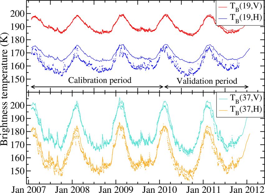
www.the-cryosphere.net/13/1215/2019/ The Cryosphere, 13, 1215–1232, 20191224 N. Champollion et al.: Decrease in the snow density near the surface at Dome C
ber 2011 (when all datasets are available), the mean surface sity of the first 3–5 m of snow at Dome C, which is about
snow density is 339.8 ± 58.8, 304.2 ± 48.7, 346.4 ± 43.9 and 350–360 kg m−3 with a range between 250–260 and 480–
303.4 ± 57.6 kg m−3 , respectively, for the satellite, CALVA 490 kg m−3 (Frezzotti et al., 2005; Brucker et al., 2011; Ver-
measurements, PNRA stake, and PNRA pit measurements. faillie et al., 2012; Groot Zwaaftink et al., 2013). The time
The datasets are consistent with one another and the mean series of ρsat shows a large range of density and all its values
values are within the uncertainty range. However, we observe have frequently been observed in previous field studies.
three notable differences: (1) measurements in snow pits are Champollion et al. (2013) linked the presence of hoar
regularly lower by 35–40 kg m−3 than satellite and stake es- crystals on the snow surface and passive microwave obser-
timates, (2) spatial variability of snow density (41.6 kg m−3 ) vations. We reassess this former study here by examining
is of the same order of magnitude as the differences between the variations in the retrieved density during hoar formation
the mean value of datasets (higher difference is 43 kg m−3 ), and disappearance events from 23 November 2009 to 4 Oc-
and (3) satellite density (standard deviation is 63.5 kg m−3 ) is tober 2011. Among the 14 hoar formation events observed
generally more variable than the in situ measurements (stan- with an automatic camera in the field, ρsat decreases in 10
dard deviations are 43, 40, and 54 kg m−3 ). The last obser- of them, with an average amplitude of −49.0 kg m−3 in a
vation (3) could be the result of the approximative thickness single day. For the four remaining events, ρsat slightly in-
of the retrieved satellite surface snow density (2–5 cm) com- creases by 15.0 kg m−3 ; for the 15 hoar disappearance events
pared with the in situ measurements (about 5 cm for CALVA observed from the ground, ρsat increases as expected for 14
measurements and 10 cm for PNRA measurements). of them, with an average amplitude of +47.0 kg m−3 ; for
The four time series of surface snow density show a pluri- the remaining event, ρsat decreases by −10.0 kg m−3 . The
annual decreasing trend. The linear trends during the com- good agreement between the quick ρsat variations and hoar
mon period (February 2010 to October 2011) for the four evolution confirms the precision of the detection of density
time series are of the same order of magnitude, between changes from AMSR-E. The influence of surface properties
−20 and −40 kg m−3 yr−1 . The trend over 10 years of the on passive microwave observations has also been confirmed
satellite-retrieved density is −13 kg m−3 yr−1 and the trend in Brucker et al. (2014) and Leduc-Leballeur et al. (2017).
over 4 years of the two PNRA in situ datasets are −6 and
−8 kg m−3 yr−1 . 5.4.3 Comparison with active microwave observations
5.4.2 Comparison with existing studies The QuikSCAT 7-year time series of the residual backscatter
at vertical and horizontal polarization and the radar polariza-
Gallet et al. (2014) measured the snow density very close to tion ratio are shown in Fig. 7. The time series are smoothed
the surface and found a range of density between 125 and with a 5-day moving window in order to reduce the influ-
165 kg m−3 for the first centimetre of snow and between 202 ence of the QuikSCAT viewing angle variations. The three
and 290 kg m−3 for the second centimetre. In Gallet et al. curves feature quick variations (daily to monthly), an an-
(2011), the authors sampled the density near the surface in nual cycle (clearly visible only after 2004 for RPR time se-
snow pits (at around 2 cm depth) and found a snow density ries), and a pluri-annual trend. The linear trend of vertical
range from 146 to 325 kg m−3 . Libois et al. (2014) mea- polarized backscatter is nearly constant, whereas the time
sured the snow density near the surface between 150 and series of horizontal polarization backscatter shows a linear
360 kg m−3 . In a study dedicated to spatial variability, Pi- decrease of −0.03 dB yr−1 . The RPR time series increases
card et al. (2014) found a range of snow density from 270 by 0.0042 yr−1 , which is comparable to the observed trends
to 520 kg m−3 in the first metre of the snowpack. During the of passive microwave observations: 0.0032 yr−1 for PR37 ,
2010–2011 summer campaign at Dome C, we measured sur- 0.0033 yr−1 for PR19 , and 0.0024 yr−1 for PR10 . We can con-
face snow densities between 270 and 380 kg m−3 . We also clude from the absence of a trend in the σv0 time series that
measured the density of hoar crystals present at the surface. surface roughness has not evolved much between 2002 and
The mean value was 178 kg m−3 , in agreement with the mea- 2009 at Dome C, Antarctica. Furthermore, the negative trend
surements of hoar crystal density performed in Greenland of of the horizontal backscatter and the positive trend of RPR
150 kg m−3 (Shuman et al., 1993). All surface snow density are certainly associated with a slow decrease in surface snow
measurements are coherent together, showing lower density density since 2002, and thus QuikSCAT observations con-
values when surface snow is covered by hoar crystals (about firm the density retrieved from AMSR-E satellite.
125–178 kg m−3 ). The surface snow densities retrieved from The ENVISAT–RA-2 time series of the residual backscat-
satellite are between 136 and 508 kg m−3 . The average den- ter at 13.6 GHz is presented in Fig. 8. The time series shows
sity over the 10 years is 377 kg m−3 and the standard de- a superimposition of a negative linear trend of −0.1 dB yr−1 ,
viation is 63.5 kg m−3 . The retrieved densities are slightly an annual cycle with large amplitude (between 0.4 and
higher than those found in existing studies or those mea- 1.2 dB yr−1 ), and weekly oscillations. These latter variations
sured during the 2010–2011 summer campaign (upper bound are residual biases between ascending and descending passes
is 380 kg m−3 ). The average of ρsat is close to the mean den- and are removed by smoothing the time series. The annual
The Cryosphere, 13, 1215–1232, 2019 www.the-cryosphere.net/13/1215/2019/N. Champollion et al.: Decrease in the snow density near the surface at Dome C 1225
Figure 6. Time series of the snow density near the surface at Dome C, Antarctica, retrieved from AMSR-E passive microwave observations
and measured in the field (three different datasets) from 18 June 2002 to 4 October 2011 (a). Panel (b) focuses on the last two years, and
panel (c) focuses on the trends during the last two years.
cycles are caused by changes in the volume echo of the EN- angle, and of considering the temporal evolution of the sur-
VISAT observations (Adodo et al., 2018). face roughness and the snow deeper into the snowpack.
The pluri-annual trend of ENVISAT–RA-2 observations
of −0.1 dB yr−1 comes mainly from a progressive evolu- 5.5.1 Uncertainty assessment
tion of surface snow density or surface roughness (Sect. 3.2).
Lacroix et al. (2008, 2009) quantified the influence of indi- We use here the signal-to-noise ratio (SNR) to characterize
vidual snow parameters on radar backscatter by modelling the significance of our results. SNR is the ratio between the
the waveform of the altimetric signal. We use the relationship mean of the observed data over the standard deviation of the
found by Lacroix et al. (2008, 2009) to convert backscat- background noise. In our time series of surface snow den-
ter coefficient changes to surface snow density variations: sity, we assume that the standard deviation of quick varia-
for a smooth surface, a surface snow density increase of tions to be noise even though part of it may be a natural
100 kg m−3 results in a backscatter coefficient increase of signal. That gives an upper limit of the noise. We found
0.3 dB at Ku band. It results in an estimation of the surface a SNR of 5.9. This value is high enough to conclude that
snow density decrease from ENVISAT–RA-2 observations of a real signal emerges from the noise, and thus the nega-
around −30 kg m−3 yr−1 , which is about 2.3 times larger in tive trend of surface snow density is significant at Dome C.
amplitude than the trend found from AMSR-E observations. Furthermore, the spatial variability of surface snow density
(41.6 kg m−3 ) was measured near Concordia Station, which
is smaller than the standard deviation of the retrieved density
5.5 Uncertainties and discussion (63.5 kg m−3 ). That indicates that variations in the retrieved
density are not only due to the spatial variability. However,
We first present an assessment of the uncertainties and then the spatial variability is not directly taken into account in
discuss the importance of several caveats that may affect the the retrieved density. This results in uncertainties in the re-
accuracy of ρsat : the effects of using a constant vertical pro- trieved density (Brucker et al., 2011; Picard et al., 2014). In
file of temperature, of variations of the azimuthal viewing the last study, the authors found an alternation every 15–25 m
www.the-cryosphere.net/13/1215/2019/ The Cryosphere, 13, 1215–1232, 20191226 N. Champollion et al.: Decrease in the snow density near the surface at Dome C
Figure 9. Time series of the snow density near the surface ρsat at
Dome C, Antarctica, retrieved from AMSR-E passive microwave
observations and covering the period from 1 December 2006 to
4 October 2011: (black dots) using the temperature profile of each
day and (solid grey line) using a temperature profile that is constant
over time.
of dense and hard snow and light and loose snow areas. They
found smaller density variations at larger scales which indi-
cate that the spatial variability of density exists at smaller
scales than the AMSR-E satellite pixel (625 km2 ). They con-
clude that changes in emissivity, as observed by Lacroix et al.
(2009), might be solely due to changes in the proportion of
dense and hard snow features without significant changes in
surface properties. In this study, we conclude that the de-
Figure 7. Time series of the residual vertical and horizontal crease in surface snow density can not be solely due to a
backscattering coefficients and the radar polarization ratio from decrease in the proportion of dense and hard snow features
QuikSCAT at Dome C, Antarctica, from 18 June 2002 to 23 Novem- because the trend is observed in other datasets which have
ber 2009. Grey lines are the original data and red, blue, and black
very different spatial scales, from a scale of a few metres for
dots are the 5-day moving averages. Note the different vertical axis
scales for horizontal polarization (H-pol) and vertical polarization
in situ measurements up to hectometre or kilometre scales
(V-pol) for active microwave observations.
5.5.2 Caveats affecting the accuracy of the retrieved
density
The vertical profile of temperature
Figure 9 shows the time series of ρsat using either the vertical
temperature profile of the day or a temperature profile that is
constant over time as used in Sect. 5.3 to retrieve the sur-
face snow density. Both curves overlap each other very well
which confirms the small influence of the temperature profile
on ρsat . This is not surprising, since we already showed the
limited influence of temperature changes of the upper layer
(Fig. 4). When considering a constant profile of temperature,
the standard deviation of the retrieved density is 59.5 kg m−3 ,
Figure 8. Time series of the backscattering coefficient from slightly higher than when the actual temperature profile of
ENVISAT–RA-2 at Dome C, Antarctica, from 12 March 2002 to each day is used (57.4 kg m−3 ). The overall trend of the re-
8 April 2012. trieved snow density is −11.2 and −10.2 kg m−3 yr−1 , re-
spectively, when using the vertical temperature profile of
each day or a constant profile of temperature.
The Cryosphere, 13, 1215–1232, 2019 www.the-cryosphere.net/13/1215/2019/N. Champollion et al.: Decrease in the snow density near the surface at Dome C 1227
The azimuthal viewing angle even though we can not conclude this definitively: (1) Long
and Drinkwater (2000) found a relatively low sensitivity of
If satellite observations were performed over an isotropic sur- the polarization ratio to surface roughness; (2) the surface
face, the azimuth angle would have no effect on the mea- roughness is mainly governed by wind and, during the last
surements. This is not the case over the Antarctic Plateau, decade, no clear wind evolution was found; and (3) most of
as many studies demonstrated the effect of azimuthal varia- the time, the lower the frequency, the higher the sensitivity
tion on satellite measurements (Fung and Chen, 1981; Tsang, of active microwave observations to surface roughness. This
1991; Shuman et al., 1993; Li et al., 2008; Narvekar et al., relationship is unclear for AMSR-E observations due to the
2010). However, this effect is weak in our study because difference of zenith viewing angle (Tsang, 1991; Liang et al.,
we use daily averaged observations and the first two compo- 2009). However, we should observe a frequency dependence
nents of the Stokes vector that minimize the effect of vari- of the polarization ratio evolution if the surface roughness
ations in the azimuthal viewing angle (Long et al., 2001; has evolved with time, at least for small-scale roughness. Yet,
Li et al., 2008; Narvekar et al., 2010). Furthermore, pas- the PR trends from AMSR-E are 0.00319 and 0.00326 at, re-
sive microwaves are less sensitive than active microwaves spectively, 37 and 19 GHz, which is thus compatible with a
to the azimuth viewing angle of the observations (Ulaby limited evolution of the small-scale roughness. Concerning
et al., 1981). Lastly, the surface is flat around Dome C, the large-scale topography around Dome C, the minor im-
lower than 1 m km−1 (Rémy et al., 1999), and thus the effect pact on satellite observations has been previously discussed.
of azimuthal variations in the surface roughness on bright-
ness temperature remains limited (Rémy and Parouty, 2009; The snow at depth
Narvekar et al., 2010).
The snow below the top layer up to few metres depth in-
The surface roughness fluences the polarization ratio through internal reflections.
Changes in volume scattering (due to snow grains), caused
The roughness of the snow surface has a direct influence on by the evolution of snow deeper into the snowpack, certainly
passive and active microwave observations (Rémy and Min- have a negligible direct effect on the retrieved density. How-
ster, 1991; Shuman et al., 1993; Flament and Rémy, 2012; ever, snow evolution can change the penetration depth of the
Rémy et al., 2014; Adodo et al., 2018). Surface roughness microwave emissions and consequently change the number
ranges from ice sheet topography (100 km wavelength) and of snow–snow interfaces caused by abrupt changes in the
large dune fields (1 to 10 km wavelength) to small features snow density profile. Interface reflections are nearly indepen-
on the surface, from millimetre to metre scales (hoar crys- dent of the wavelength according to Fresnel coefficients. The
tals and sastrugi, Shuman et al., 1993; Long and Drinkwater, influence on ρsat of snow changes deeper into the snowpack
2000; Libois et al., 2014). Our method requires the surface should thus be independent of the frequency. We consider
roughness to have a negligible effect, and thus we discuss an extreme case where the density stratification is always in-
this assumption first for active observations and then for pas- creasing with the decrease in surface snow density, keeping
sive observations. other snow parameters constant. The amount of internal re-
The radar backscatter is often reduced by an increase in flections influences the PR more than the amplitude of the
the surface roughness. The slopes of the large-scale topogra- density difference between two layers. In addition, surface
phy around Dome C are small enough, less than 1 m km −1 , reflection is at least 4–5 times higher than internal reflections
to only have a minor impact of the radar backscatter (Fla- (Fig. 10). The case considered here (increase in density strat-
ment and Rémy, 2012). The pluri-annual trend can, however, ification) leads to a decrease in the PR with time and thus
be reduced considering a rough surface (Lacroix et al., 2008; an increase in the retrieved surface snow density. As a result,
Adodo et al., 2018). Nevertheless, even with a lesser negative the trend of the retrieved density can be reduced by an in-
trend, ENVISAT and QuikSCAT observations confirm the crease in the snow density stratification. However, this effect
decrease in the surface snow density observed at Dome C by probably remains small because changing the density of the
AMSR-E with completely independent data. QuikSCAT ob- second layer from 200 to 400 kg m−3 involves changes in the
servations also suggest a slow evolution of the surface rough- relationship between ρsat and PR37 lower than 20 % (Fig. 10).
ness. Furthermore, changing the snow density of the third layer re-
Concerning passive microwave observations, as discussed sults in an influence on the PR slope of less than 10 %. As
in Champollion et al. (2013), the surface roughness influence a result, decreasing the snow density of the second layer by
is higher at vertical polarization than at horizontal polariza- 10 kg m−3 (which is the trend of the retrieved density) has a
tion. The surface roughness tends to increase the polarization weak influence on PR at 37 GHz. Finally, modelling the evo-
ratio and reduce the retrieved density. As a result, the trend of lution of the density profile is needed to definitively quantify
the retrieved surface snow density can be reduced by an in- its effect on the retrieved surface snow density. However, the
crease in the surface roughness with time. The following rea- sign of the trend will remain negative and the order of mag-
sons argue in favour of a small effect of the surface roughness nitude will probably remain the same.
www.the-cryosphere.net/13/1215/2019/ The Cryosphere, 13, 1215–1232, 2019You can also read