Slow feedbacks resulting from strongly enhanced atmospheric methane mixing ratios in a chemistry-climate model with mixed-layer ocean
←
→
Page content transcription
If your browser does not render page correctly, please read the page content below
Atmos. Chem. Phys., 21, 731–754, 2021
https://doi.org/10.5194/acp-21-731-2021
© Author(s) 2021. This work is distributed under
the Creative Commons Attribution 4.0 License.

Slow feedbacks resulting from strongly enhanced atmospheric
methane mixing ratios in a chemistry–climate model with
mixed-layer ocean
Laura Stecher1 , Franziska Winterstein1 , Martin Dameris1 , Patrick Jöckel1 , Michael Ponater1 , and Markus Kunze2
1 Deutsches   Zentrum für Luft- und Raumfahrt (DLR), Institut für Physik der Atmosphäre, Oberpfaffenhofen, Germany
2 Freie   Universität Berlin, Institut für Meteorologie, Berlin, Germany

Correspondence: Laura Stecher (laura.stecher@dlr.de)

Received: 28 May 2020 – Discussion started: 26 June 2020
Revised: 14 October 2020 – Accepted: 27 October 2020 – Published: 19 January 2021

Abstract. In a previous study the quasi-instantaneous             the in situ source of water vapour through CH4 oxidation.
chemical impacts (rapid adjustments) of strongly enhanced         However, in the lower stratosphere water vapour increases
methane (CH4 ) mixing ratios have been analysed. How-             more strongly when tropospheric warming is accounted for,
ever, to quantify the influence of the respective slow cli-       enlarging its overall radiative impact. The response of the
mate feedbacks on the chemical composition it is neces-           stratosphere adjusted temperatures driven by slow climate
sary to include the radiation-driven temperature feedback.        feedbacks is dominated by these increases in stratospheric
Therefore, we perform sensitivity simulations with doubled        water vapour as well as strongly decreased ozone mixing
and quintupled present-day (year 2010) CH4 mixing ratios          ratios above the tropical tropopause, which result from en-
with the chemistry–climate model EMAC (European Centre            hanced tropical upwelling.
for Medium-Range Weather Forecasts, Hamburg version –                While rapid radiative adjustments from ozone and strato-
Modular Earth Submodel System (ECHAM/MESSy) Atmo-                 spheric water vapour make an essential contribution to the
spheric Chemistry) and include in a novel set-up a mixed-         effective CH4 radiative forcing, the radiative impact of the re-
layer ocean model to account for tropospheric warming.            spective slow feedbacks is rather moderate. In line with this,
   Strong increases in CH4 lead to a reduction in the hy-         the climate sensitivity from CH4 changes in this chemistry–
droxyl radical in the troposphere, thereby extending the CH4      climate model set-up is not significantly different from
lifetime. Slow climate feedbacks counteract this reduction in     the climate sensitivity in carbon-dioxide-driven simulations,
the hydroxyl radical through increases in tropospheric wa-        provided that the CH4 effective radiative forcing includes the
ter vapour and ozone, thereby dampening the extension of          rapid adjustments from ozone and stratospheric water vapour
CH4 lifetime in comparison with the quasi-instantaneous re-       changes.
sponse.
   Changes in the stratospheric circulation evolve clearly
with the warming of the troposphere. The Brewer–Dobson
circulation strengthens, affecting the response of trace gases,   1   Introduction
such as ozone, water vapour and CH4 in the stratosphere, and
also causing stratospheric temperature changes. In the mid-       Methane (CH4 ) is the second-most important greenhouse gas
dle and upper stratosphere, the increase in stratospheric wa-     (GHG) directly emitted by human activity. Apart from its di-
ter vapour is reduced with respect to the quasi-instantaneous     rect radiative impact (RI), CH4 is chemically active and in-
response. We find that this difference cannot be explained        duces chemical feedbacks relevant for climate and air qual-
by the response of the cold point and the associated wa-          ity. Through its most important tropospheric sink, the oxida-
ter vapour entry values but by a weaker strengthening of          tion with the hydroxyl radical (OH), it affects the oxidation
                                                                  capacity of the atmosphere and thus its own lifetime (e.g.

Published by Copernicus Publications on behalf of the European Geosciences Union.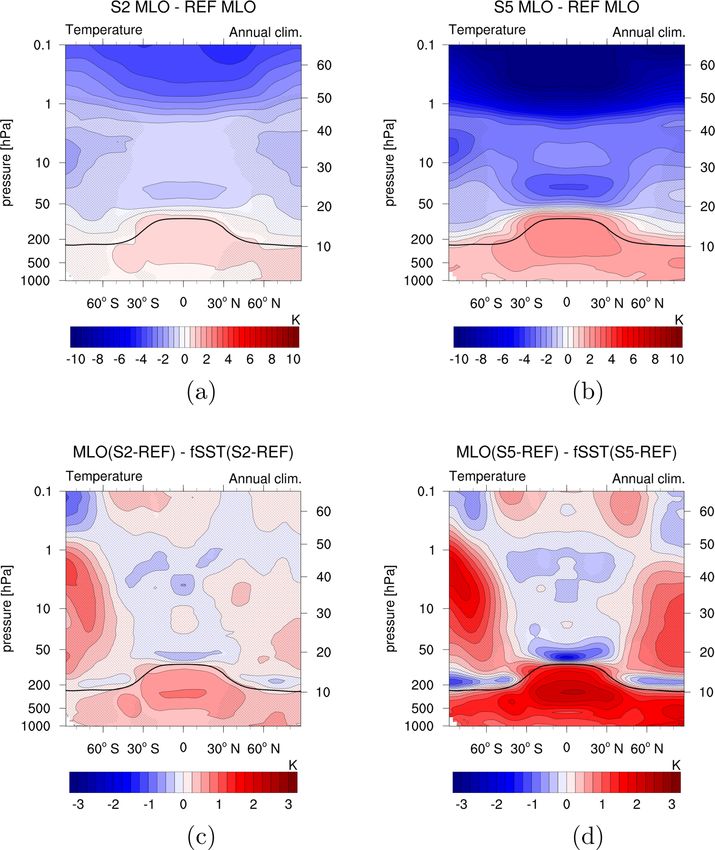
732                                                       L. Stecher et al.: Slow feedbacks from strongly enhanced methane

Saunois et al., 2016b; Voulgarakis et al., 2013; Winterstein      ice concentrations (SICs) and thus suppressed surface tem-
et al., 2019). CH4 oxidation is further an important source of    perature changes, the parameter changes in their simulations
stratospheric water vapour (SWV) (e.g. Frank et al., 2018)        match the rapid adjustment and ERF concept (e.g. Forster
and affects the ozone (O3 ) concentration in troposphere and      et al., 2016; Smith et al., 2018). Rapid radiative adjustments
stratosphere via secondary feedbacks. Chemical feedbacks          to stratospheric O3 and water vapour (H2 O) changes were
from O3 and SWV contribute significantly to the total RI in-      found to make a considerable contribution to the CH4 ERF,
duced by CH4 (e.g. Fig. 8.17 in IPCC, 2013, derived from          in line with previous respective findings (e.g. Shindell et al.,
Shindell et al., 2009 and Stevenson et al., 2013; Winterstein     2005, 2009; Stevenson et al., 2013). SWV mixing ratios were
et al., 2019). The abundance of CH4 in the atmosphere is          found to increase steadily with height under increased CH4 in
rising rapidly at present (e.g. Nisbet et al., 2019). Further-    the quasi-instantaneous response as analysed by Winterstein
more, emissions from natural CH4 sources can be prone to          et al. (2019). Rapid adjustments of the chemical composi-
climate change and have the potential to strongly enhance at-     tion of the stratosphere lead to increases in OH, favouring
mospheric CH4 concentrations (Dean et al., 2018). Together        the depletion of CH4 , which is an important in situ source
with its relevance as a GHG, the latter underlines the impor-     of SWV. The increased SWV mixing ratios cool the strato-
tance of examining implications of strongly increased CH4         sphere, thereby affecting O3 . In the troposphere, the en-
abundances in the atmosphere.                                     hanced CH4 burden leads to a strong reduction in its most
   Chemistry–climate models (CCMs) are useful tools for           important sink partner, OH, thereby affecting the CH4 life-
such studies. A CCM is a general circulation model that is        time. Winterstein et al. (2019) found a near-linear prolonga-
interactively coupled to a comprehensive chemistry module.        tion of the tropospheric CH4 lifetime with increasing scaling
This online two-way coupling is necessary to assess, on the       factor of CH4 for the two conducted experiments (2 × and
one hand, chemically induced changes in radiatively active        5 × CH4 ).
gases and their feedback on temperature and on the other             As a follow-up to Winterstein et al. (2019), we assess
hand feedbacks on chemical processes driven by changes in         the respective slow SST-driven response of the chemical
the climatic state (e.g. temperature, circulation, or precipi-    composition and resulting radiative feedbacks. Consistent
tation). A range of CCM studies analysed the sensitivity of       with Winterstein et al. (2019), we perform sensitivity sim-
other atmospheric constituents, such as O3 (Kirner et al.,        ulations with 2 × and 5 × present-day CH4 mixing ratios
2015; Morgenstern et al., 2018) and SWV (Revell et al.,           with the European Centre for Medium-Range Weather Fore-
2016) as well as OH and the CH4 lifetime (Voulgarakis et al.,     casts, Hamburg version – Modular Earth Submodel System
2013), to different projections of CH4 mixing ratios. How-        (ECHAM/MESSy) Atmospheric Chemistry model (EMAC;
ever, these studies did not focus on the climate impact of        Jöckel et al., 2016) but this time coupled to a mixed-layer
CH4 .                                                             ocean (MLO) model instead of prescribing SSTs and SICs.
   In climate feedback and sensitivity studies it has become      For RF strengths as discussed here, equilibrium climate sen-
standard to distinguish between rapid adjustments of the sys-     sitivity simulations using a thermodynamic MLO as a lower
tem (that develop in direct reaction to the forcing, inde-        boundary condition have been shown to represent the sur-
pendently from sea surface temperature (SST) changes) and         face temperature response yielded in (much more resource-
feedbacks driven by slowly evolving temperature changes at        demanding) model set-ups involving a dynamic deep ocean
the Earth’s surface (e.g. Colman and McAvaney, 2011; Ge-          sufficiently well (e.g. Danabasoglu and Gent, 2009; Dunne
offroy et al., 2014; Smith et al., 2020). Under this concept,     et al., 2020; Li et al., 2013). The slow feedbacks are assessed
the rapid radiative adjustments are counted as an integral part   as the difference between the full response (as simulated in
of the radiative forcing (RF), yielding the so-called effective   the MLO simulations) and the rapid adjustments (as simu-
radiative forcing (ERF) (Shine et al., 2003; Hansen et al.,       lated in the simulations with prescribed SSTs and SICs). To
2005). The concept has been found to be physically more           our knowledge, this is the first study assessing the response
meaningful than other RF frameworks because the climate           to strong increases in CH4 mixing ratios in a fully coupled
sensitivity parameter, i.e. the global mean surface tempera-      CCM, meaning that the interactive model system includes at-
ture change per unit RF, is becoming less dependent on the        mospheric dynamics, atmospheric chemistry, and ocean ther-
forcing agent (Hansen et al., 2005; Sherwood et al., 2015;        modynamics.
Richardson et al., 2019). However, recent studies of climate         Our simulation strategy is explained in Sect. 2. The dis-
feedbacks and sensitivity to a CH4 forcing adopting the ERF       cussion of results in Sect. 3 starts with a brief evaluation
concept did not account for the radiative contribution from       of the reference CH4 mixing ratio against observations and
chemical feedbacks in their analysis (Modak et al., 2018;         an assessment of the MLO model (Sect. 3.1), followed by
Smith et al., 2018; Richardson et al., 2019).                     the analyses of tropospheric warming and associated climate
   Winterstein et al. (2019) assessed chemical feedback pro-      feedbacks in the MLO simulations (Sect. 3.2). In Sect. 3.3
cesses and their RI in simulations forced by doubled (2×)         we assess implications of SST-driven climate feedbacks on
and quintupled (5×) present-day (year 2010) CH4 mixing ra-        the chemical composition of the atmosphere in comparison
tios. As their simulation set-up used prescribed SSTs and sea     to the quasi-instantaneous response and quantify the result-

Atmos. Chem. Phys., 21, 731–754, 2021                                                https://doi.org/10.5194/acp-21-731-2021
L. Stecher et al.: Slow feedbacks from strongly enhanced methane                                                            733

ing radiative feedbacks and the climate sensitivity. We fur-     are prescribed by Newtonian relaxation (i.e. nudging) with a
ther discuss contributions from feedbacks of radiatively ac-     nudging coefficient of 10 800 s. Thus, no CH4 emission flux
tive gases and from circulation changes to the stratosphere      boundary was used, but pseudo surface fluxes were calcu-
temperature response. In Sect. 4 we summarize our conclu-        lated by the MESSy submodel TNUDGE (Kerkweg et al.,
sions and give a brief outlook.                                  2006) to reach the prescribed CH4 lower-boundary mixing
                                                                 ratios. The lower-boundary CH4 mixing ratios of REF MLO
                                                                 are nudged to the same reference as REF fSST, namely
2   Description of the model and simulation strategy             an observation-based zonal mean estimate of the year 2010
                                                                 from marine boundary-layer sites. The observational data are
We use the CCM ECHAM/MESSy Atmospheric Chemistry                 provided by the Advanced Global Atmospheric Gases Ex-
(EMAC; Jöckel et al., 2016) for this study. Following on         periment (AGAGE; http://agage.mit.edu/, last access: 9 De-
from the sensitivity simulations with prescribed SSTs and        cember 2020) and the National Oceanic and Atmospheric
SICs that were analysed by Winterstein et al. (2019), we         Administration Earth System Research Laboratory (NOAA-
performed a second set of sensitivity simulations with the       ESRL; https://www.esrl.noaa.gov/, last access: 9 December
MESSy submodel MLOCEAN (Kunze et al., 2014; origi-               2020). The lower-boundary CH4 mixing ratios of S2 and S5
nal code by Roeckner et al., 1995) coupled to EMAC. The          are nudged towards the 2× and the 5× of this reference, re-
set-up of the MLO simulations is designed to follow the          spectively. The resulting global mean lower-boundary CH4
set-up of the simulations described by Winterstein et al.        mixing ratio is about 1.8 parts per million volume (ppm) for
(2019) closely. We conducted all simulations at a resolution     both reference simulations, 3.6 ppm for both doubling, and
of T42L90MA, corresponding to a quadratic Gaussian grid          9.0 ppm for both quintupling experiments. Apart from CH4 ,
of approximately 2.8◦ × 2.8◦ resolution in latitude and lon-     all other boundary conditions and emission fluxes used in the
gitude and 90 levels, with the uppermost level centred around    sensitivity simulations are identical to the reference simula-
0.01 hPa in the vertical.                                        tions and represent conditions of the year 2010 in general.
   According to the simulation concept of Winterstein et al.        In the MLO simulations, the SSTs, the ice thicknesses, and
(2019), we performed one reference simulation (REF MLO)          the ice temperatures at ocean grid points are calculated by the
and two sensitivity simulations (S2 MLO and S5 MLO) in-          MESSy submodel MLOCEAN. A MLO model accounts for
cluding the MLO model, all as equilibrium climate simula-        the ocean’s heat capacity without simulating the oceanic cir-
tions. The simulations with prescribed SSTs and SICs are de-     culation explicitly. To simulate realistic SSTs with the MLO,
noted REF fSST, S2 fSST, and S5 fSST here. All simulations       a heat flux correction term needs to be added to the surface
considered for the analysis are listed in Table 1. The MLO       energy balance. We derived a monthly climatology of this
simulations have been performed with a more recent ver-          heat flux correction from a control simulation with prescribed
sion of MESSy (2.54.0 instead of 2.52). The updates include      SSTs and SICs, named REF QFLX. REF QFLX uses the
changes in the chemistry module Module Efficiently Calcu-        same monthly climatology of SSTs and SICs that was used
lating the Chemistry of the Atmosphere (MECCA; Sander            for the fSST simulations, i.e. a monthly climatology repre-
et al., 2011) that are discussed in Appendix A. However, in-     senting the years 2000 to 2009 based on global analyses of
herent differences between the MLO and fSST simulations          the HadISST1 data set (Rayner et al., 2003).
do not directly distort the evaluation as the differences be-       In the following, the response to increased CH4 in the
tween response signals relative to the respective reference      MLO simulations is assessed as the difference between ei-
simulations and not the direct differences between the sen-      ther S2 MLO or S5 MLO and REF MLO. The effects of SST-
sitivity simulations are analysed.                               driven climate feedbacks are identified as the difference be-
   A spin-up phase of at least 10 years is excluded from         tween responses in the MLO and fSST simulations. The RIs
the analysis of each simulation to provide quasi-steady-state    induced by changes in individual radiatively active gases are
conditions. S2 MLO and S5 MLO were initialized from the          assessed using the EMAC option for multiple radiation calls
spun-up state of REF MLO and spun-up over a 10-year pe-          in the submodel RAD (Dietmüller et al., 2016), as explained
riod followed by a 20-year equilibrium used for the analysis.    in more detail by Winterstein et al. (2019). The first radia-
We chose to simulate a 30-year equilibrium for the analysis      tion call receives the reference mixing ratios of all chemical
of REF MLO after S2 MLO and S5 MLO branched off so               species, i.e. CH4 , O3 , and H2 O. In the following radiation
that the complete 20 years used for the analysis of S2 MLO       calls, each of the species individually and all combined are
and S5 MLO are covered by this simulation as well.               exchanged by climatological means derived from the sensi-
   The MLO simulations have been initialized with the equi-      tivity simulations (S2 and S5). From these perturbed radia-
librium CH4 fields of the respective fSST simulations. As        tion fluxes, the stratosphere adjusted RI is calculated (Stuber
the latter are already close to the respective equilibrium CH4   et al., 2001; Dietmüller et al., 2016).
fields of the MLO simulations, the initialization with these
fields shortens the spin-up. Like the fSST simulations, the
CH4 lower-boundary mixing ratios of the MLO simulations

https://doi.org/10.5194/acp-21-731-2021                                             Atmos. Chem. Phys., 21, 731–754, 2021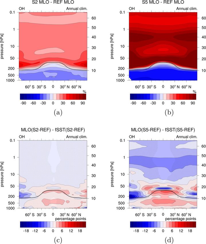
734                                                          L. Stecher et al.: Slow feedbacks from strongly enhanced methane

Table 1. Overview of the two sets of sensitivity simulations (fSST and MLO) with one reference simulation and two sensitivity simulations.
The simulations with prescribed SSTs and SICs have already been analysed by Winterstein et al. (2019). The simulation REF QFLX is used
to determine the heat flux correction for the simulations including the MLO model.

                        Simulation     CH4 lower boundary      SSTs, SICs                         MESSy version
                        REF fSST       1.8 ppmv
                        S2 fSST        2 × REF fSST            prescribed (Rayner et al., 2003)              2.52
                        S5 fSST        5 × REF fSST
                        REF MLO        1.8 ppmv                mixed-layer ocean (MLO)
                        S2 MLO         2 × REF MLO             MESSy submodel MLOCEAN                      2.54.0
                        S5 MLO         5 × REF MLO
                        REF QFLX       1.8 ppmv                prescribed (Rayner et al., 2003)       d2.53.0.26

3     Discussion of results                                            REF MLO represents CH4 conditions of the year 2010 that
                                                                       are sufficiently realistic.
                                                                          Since this study is one of the first to use the MLOCEAN
3.1    Assessment of reference simulations
                                                                       submodel in MESSy, we have carefully checked whether
                                                                       REF MLO reproduces SSTs and SICs of the climatology that
The simulation set-up of the reference simulation,                     was used to determine the heat flux correction with sufficient
REF MLO, aims to represent conditions typical for the                  accuracy. The spatial pattern of the SST climatology is real-
year 2010. For a detailed assessment and evaluation of                 istically reproduced in REF MLO (see Fig. S1). The largest
EMAC in general, we refer to Jöckel et al. (2016). We have             differences are found at higher latitudes, where a reduction
evaluated the REF MLO CH4 mixing ratios to ensure that                 in sea ice area leads to higher SSTs as exposed seawater is
the latter represent conditions of 2010 sufficiently realisti-         warmer than sea ice. REF MLO underestimates the monthly
cally. The REF MLO CH4 mixing ratios were compared to                  climatology of sea ice area in the Southern Hemisphere (SH)
three different observational data sets that are independent           in all seasons, except for austral summer (see Fig. S2). The
from the observational estimate that serves as input for the           reduction in SIC results in up to 1.5 K higher SSTs in the
lower boundary condition to ensure an objective evaluation.            Southern Ocean in REF MLO compared to the prescribed
These are balloon-borne measurements conducted in the                  climatology (see Fig. S1). In the Northern Hemisphere (NH),
period from 1992 to 2006 from Röckmann et al. (2011),                  the annual cycle of the sea ice area is generally well repro-
observations of a portable Fourier transform spectrometer              duced (see Fig. S2), except for a slight overestimation of the
on board the research vessel Polarstern during a cruise                sea ice area in REF MLO, resulting in about 0.5 K lower an-
from Cape Town to Bremerhaven on the Atlantic in 2014                  nual mean SSTs in the Greenland Sea and in the Barents Sea
(Klappenbach et al., 2015), and observations from the Total            (see Fig. S1). However, the sign of the global and annual
Carbon Column Observing Network (TCCON; Wunch                          mean surface temperature difference between REF MLO and
et al., 2011) from the period 2009 to 2014. The vertical               REF fSST is determined by the positive REF MLO bias re-
profile, the north–south gradient and the annual cycle of              lated to the Antarctic sea ice reduction. The global mean dif-
REF MLO CH4 generally agree well with the corresponding                ference is 0.28 K, much less than the regional maxima near
data (not shown). Consistent with REF fSST (see Win-                   the ice edges, and with a small contribution of about 0.10 K
terstein et al., 2019), there is a negative bias between the           from the tropical belt. It is unlikely that this will lead to
REF MLO and the observed total CH4 columns of less                     substantial biases in the estimation of global mean surface
than 4 % (not shown). Note that not all the observations               temperature response and climate sensitivity in the intended
originate precisely from the year 2010. The global annual              equilibrium climate change simulations.
mean CH4 surface mixing ratios have, for example, risen
by about 0.024 ppm from 2010 to 2014 (NOAA/ESRL;                       3.2   Tropospheric temperature response and associated
https://www.esrl.noaa.gov/gmd/ccgg/trends_ch4/,           last               climate feedbacks
access: 9 December 2020), the year of the study by Klap-
penbach et al. (2015). In addition, the CH4 lifetime could be          The tropospheric temperature response to enhanced CH4
slightly underestimated. The CH4 lifetime in EMAC lies in              mixing ratios can freely develop in the MLO sensitivity sim-
the middle to lower range in comparison with other CCMs                ulations (see Fig. 1a, b). The temperature change patterns of
(Jöckel et al., 2006; Voulgarakis et al., 2013). However,              S2 MLO and S5 MLO show the expected warming of the tro-
given that relative comparisons between sensitivity simula-            posphere and cooling of the stratosphere (e.g. IPCC, 2013).
tions and the reference are the main target of our analysis,           The stratospheric cooling is less pronounced than in carbon

Atmos. Chem. Phys., 21, 731–754, 2021                                                       https://doi.org/10.5194/acp-21-731-2021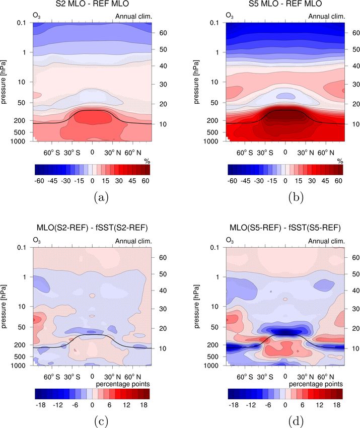
L. Stecher et al.: Slow feedbacks from strongly enhanced methane 735
dioxide (CO2 )-driven climate change simulations since the 3.3 Influence of interactive SSTs
CH4 cooling is mainly caused by associated O3 and H2 O
adjustments (Kirner et al., 2015; Winterstein et al., 2019). 3.3.1 Chemical composition
Maximum warming in polar regions and in the upper tropical
troposphere is also consistent with changes expected from in- Winterstein et al. (2019) analysed the quasi-instantaneous
creased levels of GHGs (e.g. Chap. 12 in IPCC, 2013). CH4 impact of doubled and quintupled CH4 mixing ratios on the
doubling (quintupling) leads to temperature increases of up chemical composition of the atmosphere. In this section we
to 1 K (3 K) in the Arctic on annual average. Antarctica also investigate the respective slow feedbacks that are assessed as
warms up particularly strongly in the S5 MLO scenario, with the difference between the full response (as simulated in the
a maximum warming of up to 3 K. As a result of the es- MLO simulations) and the rapid adjustments (as simulated
pecially strong warming in polar regions, the sea ice area is in the fSST simulations). The slow feedbacks are therefore
reduced in both sensitivity simulations with respect to the visualized as the differences between the response patterns
reference (compare Fig. S2). in the fSST simulations and in the MLO simulations.
The Brewer–Dobson circulation (BDC) is expected to ac-
Tropospheric CH4 lifetime and OH
celerate in a warming climate (Rind et al., 1990; Butchart
and Scaife, 2001; Garcia and Randel, 2008; Butchart, 2014; The oxidation with OH is the most important sink of CH4
Eichinger et al., 2019). Feedbacks on the chemical composi- in the troposphere (e.g. Saunois et al., 2016a). The amount
tion of the atmosphere, especially of the stratosphere, which of oxidized CH4 affects the OH mixing ratios as the reaction
result from changes in the BDC are of particular interest in consumes OH, which in turn feeds back on the atmospheric
this study as they will modify the mainly chemically induced CH4 lifetime. In this study, consistent with Winterstein et al.
changes discussed by Winterstein et al. (2019). The BDC in- (2019), the CH4 lifetime is calculated according to Jöckel
fluences the spatial distribution of trace gases, such as O3 , et al. (2016) as
H2 O, and CH4 , in the stratosphere and also their transport P
from the troposphere into the stratosphere (Butchart, 2014). mCH4
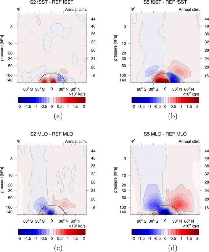
In Fig. 2 we examine the response of the residual mean b∈B
τCH4 = P , (1)
streamfunction to quantify changes in the BDC. There is in- kCH4 +OH (T ) · cair (T , p, q) · xOH · mCH4
b∈B
deed a strengthening of the residual mean circulation in both,
S2 MLO and S5 MLO, with respect to REF MLO and it is de- with mCH4 being the mass of CH4 [kg], kCH4 +OH (T ) the tem-
tected in both hemispheres. The change in the residual mean perature dependent reaction rate coefficient of the reaction
streamfunction is stronger and extends to higher altitudes for CH4 + OH → products [cm3 s−1 ], cair the concentration of
the simulation S5 MLO, but the annual mean patterns are air [cm−3 ], and xOH the mole fraction of OH [mol mol−1 ]
consistent in both MLO sensitivity simulations. The maxi- in all grid boxes b ∈ B. B is the region for which the life-
mum change of about 0.7×10⁹ kg s−1 for S5 MLO is located time should be calculated, e.g. all grid boxes below the
at about 100 hPa. Upward motion is increased in the tropics, tropopause for the mean tropospheric lifetime. For the CH4
which is balanced by an increase in downwelling between lifetime calculation a climatological tropopause, defined as
30–60◦ latitude in both hemispheres. The change in the resid- tpclim = 300–215 hPa · cos2 (φ), with φ being the latitude in
ual mean streamfunction is stronger and reaches higher alti- degrees north, is used as recommended by Lawrence et al.
tudes in the respective winter hemisphere in S5 MLO (see (2001).
Figs. S3 and S5). The BDC response in the MLO simula- Figure 3 shows the mean tropospheric CH4 lifetime of the
tions is considerably stronger than in the respective fSST sen- MLO experiments, together with the fSST experiments, de-
sitivity simulations. This is expected since the main driver pendent on the CH4 scaling factor, i.e. 1 for the reference
of changes in the BDC is tropospheric warming (Butchart, simulations, 2 for the experiments with 2 × CH4 , and 5 for
2014). We note that changes in the residual mean stream- those with 5 × CH4 . An almost linear relationship between
function below the tropical tropopause in response to CH4 the mean tropospheric CH4 lifetime and the CH4 scaling fac-
increase exhibit different patterns in the fSST and MLO sim- tor is present also in the MLO sensitivity simulations. The
ulations (see Fig. 2). Differences between the fast and the lifetime increase is, however, reduced by 0.30 a (increase
slow response of the tropospheric tropical circulation have by 2.03 a instead of 2.3 a) and 1.17 a (increase by 6.37 a in-
been noticed and discussed in CO2 increase simulations, too stead of 7.54 a) in the MLO set-up compared to fSST when
(e.g. Bony et al., 2013). However, trying to explain the origin doubling and quintupling CH4 , respectively. This weaker in-
of these tropospheric differences would be beyond the scope crease is in line with a weaker decrease in tropospheric OH
of the present paper, which focuses on stratospheric trace gas in the MLO sensitivity simulations compared to fSST as ob-
feedbacks to CH4 increase. The latter are influenced by the vious from Fig. 4c, d, which show the difference between the
more distinct strengthening of the BDC in the MLO experi- OH response in the MLO and in the fSST sensitivity simula-
ments, as we show in the next section. tions. In the troposphere this difference is hardly significant
anywhere for the 2 × CH4 experiments, whereas it is signifi-
https://doi.org/10.5194/acp-21-731-2021 Atmos. Chem. Phys., 21, 731–754, 2021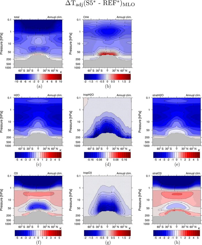
736                                                         L. Stecher et al.: Slow feedbacks from strongly enhanced methane

Figure 1. (a, b) Absolute annual zonal mean temperature differences between the sensitivity simulations (a) S2 MLO and (b) S5 MLO and
REF MLO in kelvin. (c, d) Differences between the temperature response to enhanced CH4 in the MLO and fSST set-ups in kelvin. To
calculate the latter, the absolute changes in (c) S2 fSST and (d) S5 fSST are subtracted from the absolute changes in S2 MLO and S5 MLO,
respectively. Non-stippled areas are significant on the 95 % confidence level according to a two-sided Welch’s test. The solid black line
indicates the climatological tropopause height of REF MLO.

cant in the tropics for 5 × CH4 . The weaker decrease in tro-             Voulgarakis et al. (2013) compared the CH4 lifetime
pospheric OH in both MLO simulations is related to more                increase simulated in two simulations: one with the full
strongly enhanced OH precursors (H2 O and O3 ) in the tro-             RCP8.5 climate change signal of the year 2100 with respect
posphere in the MLO compared to the fSST sensitivity simu-             to 2000 and one with CH4 concentrations corresponding to
lations, as is discussed below. Additionally, the tropospheric         2100 RCP8.5 levels but climate conditions of the year 2000.
warming in the MLO sensitivity simulations results in a                They identified a weaker increase in the CH4 lifetime with
faster CH4 oxidation as its reaction rate increases with tem-          tropospheric warming as well. Their difference is larger than
perature. The isolated effect of the temperature-dependent re-         the difference between the S2 fSST and S2 MLO lifetime
action rate is indicated by the blue squares in Fig. 3. They           responses even though the CH4 increase simulated by Voul-
show the CH4 lifetime corresponding to REF MLO condi-                  garakis et al. (2013) is of the same order of magnitude as in
tions, except for the reaction rate coefficient that was calcu-        S2 fSST and S2 MLO since the RCP8.5 scenario projects a
lated with temperatures corresponding to 2× and 5 × CH4 .              doubling of the 2010 CH4 mixing ratios at the end of the cen-
                                                                       tury. However, the tropospheric warming in the RCP8.5 sce-

Atmos. Chem. Phys., 21, 731–754, 2021                                                      https://doi.org/10.5194/acp-21-731-2021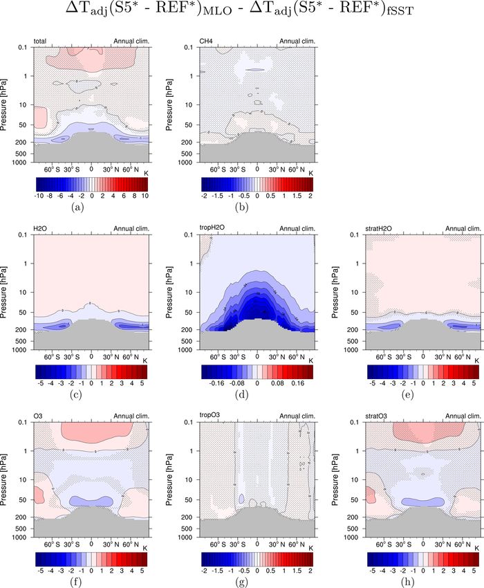
L. Stecher et al.: Slow feedbacks from strongly enhanced methane                                                                        737

Figure 2. Absolute differences in the annual zonal mean residual streamfunction between the sensitivity simulations (a) S2 fSST, (b) S5 fSST,
(c) S2 MLO, and (d) S5 MLO compared to their respective reference in 109 kg s−1 . Non-stippled areas are significant on the 95 % confidence
level according to a two-sided Welch’s test. The solid black line indicates the climatological tropopause height of REF MLO.

nario is stronger because it includes the effects of all GHGs            (2.91 ± 0.01) in the MLO simulations and by a factor of
as opposed to the isolated effect of CH4 in our experiments.             1.58 ± 0.00 (2.75 ± 0.01) in the fSST simulations (see Ta-
Additional warming induced by other GHGs, in particular                  ble 2). The larger increase factors in the MLO sensitivity sim-
CO2 , would drive H2 O and O3 increases as well. Therefore,              ulations are in line with the reduced prolongation of the tro-
the reduction in OH driven by CH4 increases in our experi-               pospheric CH4 lifetime compared to the fSST experiments.
ments is expected to be more strongly offset under a simul-              The fact that the increase in emission fluxes is less than a
taneously active CO2 forcing.                                            factor of 2 or 5 suggests that enhanced CH4 emissions would
   Please recall that we prescribe the CH4 mixing ratios at              likewise scale the mixing ratio by a larger factor than the cor-
the lower boundary using Newtonian relaxation. It is impor-              responding increase factor of the emissions. The CH4 surface
tant to note that the prolongation of the tropospheric CH4               fluxes that result from the nudging of the mixing ratio to-
lifetime causes the corresponding CH4 fluxes at the lower                wards zonally averaged CH4 fields are not realistic in terms
boundary to not scale equally with the mixing ratio increase             of spatial distribution, however.
but to increase by a smaller factor. Increasing the CH4 sur-
face mixing ratio by a factor of 2 (5) corresponds to an in-
crease in the CH4 surface fluxes by a factor of 1.61 ± 0.01

https://doi.org/10.5194/acp-21-731-2021                                                       Atmos. Chem. Phys., 21, 731–754, 2021
738 L. Stecher et al.: Slow feedbacks from strongly enhanced methane
is in line with the response of tropospheric CH4 in the fSST
simulations. Tropospheric CH4 is largely controlled by the
nudging at the lower boundary through mixing and is, there-
fore, prevented from adjusting to the lifetime increase as dis-
cussed above. The slightly positive values in Fig. 5 indicate
a small residual of this effect. As for the fSST simulations,
the CH4 increase between 50 and 1 hPa is smaller than the
factors of 2 or 5, respectively. This effect is less pronounced
in the two MLO sensitivity experiments compared to the re-
spective fSST experiments (compare with Fig. 3 in Winter-
stein et al., 2019), suggesting that the chemical depletion of
CH4 is enhanced in the MLO experiments as well, however,
less strongly than in the fSST experiments.
Another aspect to note in Fig. 5 is the more than 2× or
5×CH4 increase in the lowermost tropical stratosphere. This
feature indicates enhanced tropical upwelling, which leads to
larger CH4 mixing ratios in the tropical lower stratosphere. It
is more pronounced in the MLO than in the fSST experi-
ments, in line with the more pronounced changes in tropical
Figure 3. Mean tropospheric CH4 lifetime with respect to the ox-
upwelling in the MLO set-up as discussed in Sect. 3.2. The
idation with OH versus the scaling factor of the lower-boundary
CH4 , i.e. 1 for REF, 2 for S2, 5 for S5 for the MLO (red, dashed)
average deviation from 2× or 5 × CH4 for a region in the
and the fSST (black, solid) simulations. In addition, the isolated tropical lower stratosphere (30–30◦ N, 70–20 hPa) is 0.16 %
effect of the temperature-dependent reaction rate is shown for the for S2 fSST, 0.37 % for S2 MLO, 0.23 % for S5 fSST, and
MLO experiments (blue squares). The horizontal lines indicate the 1.31 % for S5 MLO. Furthermore, strengthening of the BDC
95 % confidence intervals based on annual mean values of the CH4 transports CH4 more efficiently to higher altitudes, leading to
tropospheric lifetime. higher CH4 mixing ratios there as well. This can be one ex-
planation for the weaker deviation from a linear CH4 increase
Table 2. Increase factors of the global mean CH4 surface fluxes, in the MLO compared to the fSST simulations. Another ex-
which correspond to increases in the CH4 mixing ratios by factors planation, as already stated, is that the chemical depletion of
of 2 or 5, respectively. The values after the ± sign are the 95 % con- CH4 is less strongly enhanced in the MLO sensitivity simula-
fidence intervals of the mean calculated using Taylor expansion (as- tions compared to fSST. We therefore discuss differences in
suming REFrfluxes to be uncorrelated with either S2 or S5 fluxes) as the response of OH, the most important sink partner of CH4 ,
sx2 sy2 in the next paragraph.
±t α ,df · xy · Nx ·x + Ny ·y , with the mean fluxes of either S2 or S5
2 Stratospheric OH mixing ratios increase in both simulation
and REF x and y, respectively; interannual standard deviations sx
set-ups (fSST and MLO) on the order of 30 % for 2 × CH4
and sy ; number of analysed years Nx and Ny ; α = 0.05; and the de-
2 2 −1 and 60 %–80 % for 5 × CH4 (see Fig. 4 in Winterstein et al.,
2
sx2 sy
2019, for fSST and Fig. 4a, b for MLO). The OH increase
2 s 2 Nx Ny
s
grees of freedom df = Nx + Ny ·
x y N −1 x
+ N −1 .
y
in the stratosphere is weaker in the MLO simulations com-
pared to the fSST simulations (see Fig. 4c, d). The differ-
ences are, however, small compared to the total increase in
OH and mainly not significant. The difference between the
fSST MLO
two 5 × CH4 experiments reaches up to 5 percentage points
S2 1.58 ± 0.00 1.61 ± 0.01 (p.p.) in the middle stratosphere. The weaker increases in
S5 2.75 ± 0.01 2.91 ± 0.01 OH are presumably connected to weaker increases in SWV
in the MLO simulations. The considerably weaker OH in-
crease above the tropical tropopause in S5 MLO with respect
Non-linearities of CH4 increase to S5 fSST is possibly associated with a stronger O3 decrease
in this area in S5 MLO. Changes in both SWV and O3 are
Figure 5 shows the relative differences between the annual discussed below. The weaker OH increases in the MLO sen-
zonal mean CH4 of S2 MLO (S5 MLO) and 2× (5×) the sitivity experiments with respect to fSST are in line with the
zonal mean CH4 of REF MLO. The doubling or quintupling smaller deviations from a linear doubling or quintupling of
of the reference CH4 serves to emphasize regions where the the CH4 mixing ratio in the stratosphere (see Fig. 5). We con-
increase factor of the CH4 mixing ratio deviates from 2 or 5, clude that the strengthening of the CH4 oxidation resulting
respectively. The response of tropospheric CH4 is marginally from increases in the OH mixing ratio is weaker in the MLO
larger than a linear increase in both MLO experiments. This experiments but still present.
Atmos. Chem. Phys., 21, 731–754, 2021 https://doi.org/10.5194/acp-21-731-2021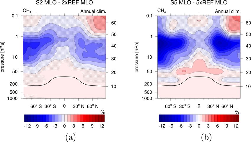
L. Stecher et al.: Slow feedbacks from strongly enhanced methane 739
Figure 4. (a, b) Relative differences between the annual zonal mean OH mixing ratios of the sensitivity simulations (a) S2 MLO and (b) S5
MLO and REF MLO (%). (c, d) Differences between the OH response to enhanced CH4 in the MLO and fSST set-ups (percentage points).
To calculate the latter, the relative changes in (c) S2 fSST and (d) S5 fSST are subtracted from the relative changes in S2 MLO and S5
MLO, respectively. Non-stippled areas are significant on the 95 % confidence level according to a two-sided Welch’s test. The solid black
line indicates the climatological tropopause height of REF MLO.
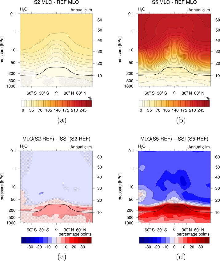
Water vapour In the middle and upper stratosphere, the H2 O increase
is about 5 p.p. (15 p.p.) weaker in the S2 MLO (S5 MLO)
sensitivity simulation compared to S2 fSST (S5 fSST). This
Winterstein et al. (2019) reported a steady increase in SWV reduction is significant but small compared to the relative in-
with height for the fSST experiments as an outcome of the crease in SWV of around 50 % for both 2 × CH4 and 250 %
enhanced CH4 depletion as discussed in the previous para- for both 5 × CH4 experiments. The amount of tropospheric
graph, whereas tropospheric H2 O remained largely unaf- H2 O transported into the stratosphere is largely determined
fected. The warming of the troposphere in the MLO simu- by the cold point temperature (CPT) (e.g. Randel and Park,
lations consistently leads to an increase in the H2 O mixing 2019). Furthermore, the oxidation of CH4 is an important in
ratios also in the troposphere as evident from Fig. 6. The situ source of SWV (Hein et al., 2001; Rohs et al., 2006;
maximum difference in tropospheric H2 O response between Frank et al., 2018). The SWV mixing ratio at a given loca-
MLO and fSST can be found in the upper tropical tropo- tion and time can be approximated as the sum of these two
sphere and extratropical lowermost stratosphere and reaches terms following Austin et al. (2007) and Revell et al. (2016)
11 p.p. (35 p.p.) for the 2× (5×) CH4 experiments.
https://doi.org/10.5194/acp-21-731-2021 Atmos. Chem. Phys., 21, 731–754, 2021740 L. Stecher et al.: Slow feedbacks from strongly enhanced methane
Figure 5. Relative differences between the annual zonal mean CH4 of the sensitivity simulations (a) S2 MLO and 2× REF MLO and
(b) S5 MLO and 5× REF MLO (%). Non-stippled areas are significant on the 95 % confidence level according to a two-sided Welch’s test.
The solid black line indicates the climatological tropopause height of REF MLO.
as ficiently and would be expected to lead to higher rates of
the CH4 oxidation (Austin et al., 2007). However, as the
H2 O = H2 Oentry + H2 OCH4 . (2) strengthening of the CH4 oxidation is weaker in the MLO
We calculate the amount of tropospheric H2 O entering the experiments, CH4 itself seems not to be the limiting factor
stratosphere as the tropical (10◦ S–10◦ N) mean H2 O mix- here. The abundance of SWV feeds back on OH and there-
ing ratio at 70 hPa following Revell et al. (2016). The fore also on the efficiency of the CH4 oxidation. However, the
H2 O entry mixing ratio increases by 9.08 % (0.14 ppm) in increase in SWV seems to be rather a result of the strength-
S2 fSST, 9.77 % (0.17 ppm) in S2 MLO, 38.53 % (0.57 ppm) ened CH4 oxidation here as the increase in H2 O entering the
in S5 fSST, and 38.86 % (0.68 ppm) in S5 MLO. Further- stratosphere is higher in the MLO experiments compared to
more, the zonal mean tropical CPT increases in all sensitivity fSST.
simulations (see Fig. S7). Though differences exist between
the reference CPT in MLO und fSST, the magnitude and lat- Ozone
itudinal structure of the CPT changes are very similar for
both doubling and both quintupling experiments. They are The other important precursor of OH is O3 , the abundance
also a bit larger for the MLO experiments (again consistent of which is also influenced by CH4 . The stratospheric O3
for the S2 and S5 case), in line with the response of the H2 O response pattern in the MLO experiments, namely O3 reduc-
entry mixing ratios. Changes in the amount of tropospheric tion in the lowermost tropical stratosphere, O3 increase up
H2 O entering the stratosphere can therefore not explain the to approximately 2 hPa, and O3 decrease above, is qualita-
weaker increase in SWV in the MLO experiments compared tively consistent with the fSST simulations (compare Fig. 7
to fSST in the middle and upper stratosphere. in Winterstein et al., 2019, and Fig. 7a, b). Winterstein et al.
To illustrate the effect of CH4 oxidation on the SWV re- (2019) gave a detailed explanation of the processes leading
sponse, Fig. S8 shows the response of H2 O from CH4 ox- to the resulting O3 pattern that is also valid for the MLO
idation estimated using Eq. (2). As discussed in the previ- simulations. As the O3 catalytic depletion cycles are less ef-
ous paragraph, the strengthening of the CH4 oxidation in the ficient at lower temperatures, radiative cooling in the strato-
stratosphere is weaker in the MLO experiments. This results sphere results in increased O3 mixing ratios in the middle
in a weaker increase in SWV produced by CH4 oxidation in stratosphere (between 50 and 5 hPa). Additionally, increased
the middle and upper stratosphere (see Fig. S8c, d) and can abundances of H2 O favour the depletion of excited oxygen
explain the difference in SWV response between MLO and (O(1 D)), likewise reducing the sink of O3 and favouring in-
fSST as shown in Fig. 6c, d. creases in the O3 abundance. Reduced O3 mixing ratios in
What remains to be explained is the reason for the weaker the lowermost tropical stratosphere indicate enhanced trop-
strengthening of the CH4 oxidation in the MLO set-up com- ical upwelling of O3 -poor air from the troposphere into the
pared to fSST. Strengthened tropical upwelling as shown stratosphere. Above 2 hPa, increases in OH lead to enhanced
in Sect. 3.2 transports CH4 into the stratosphere more ef- depletion of O3 , resulting in reduced O3 mixing ratios.
Atmos. Chem. Phys., 21, 731–754, 2021 https://doi.org/10.5194/acp-21-731-2021L. Stecher et al.: Slow feedbacks from strongly enhanced methane 741 Figure 6. (a, b) Relative differences between the annual zonal mean H2 O mixing ratios of the sensitivity simulations (a) S2 MLO and (b) S5 MLO and REF MLO (%). (c, d) Differences between the H2 O response to enhanced CH4 in the MLO and fSST set-ups (percentage points). To calculate the latter, the relative changes in (c) S2 fSST and (d) S5 fSST are subtracted from the relative changes in S2 MLO and S5 MLO, respectively. Non-stippled areas are significant on the 95 % confidence level according to a two-sided Welch’s test. The solid black line indicates the climatological tropopause height of REF MLO. When subtracting the fSST response from the MLO re- MLO simulations. The increases in O3 in the southern polar sponse, the extra effect of tropospheric warming becomes middle stratosphere in S2 MLO and in both polar regions apparent. The resulting patterns for S2 and S5 are shown in in S5 MLO are more pronounced with respect to the respec- Fig. 7c, d. A dominant feature is the stronger decrease in O3 tive fSST experiment. This indicates more strongly enhanced in the lowermost tropical stratosphere in S5 MLO compared meridional transport in the MLO experiments. Both patterns to S5 fSST of up to 18.39 p.p. The average difference be- are in line with the strengthening of the residual mean circu- tween S5 MLO and S5 fSST for a region in the tropical lower lation as discussed in Sect. 3.2. stratosphere (30◦ S–30◦ N, 100–20 hPa) is 6.33 p.p. This dif- In the tropospheric O3 response pattern (shown in ference also exists between the S2 simulations, albeit weaker Fig. 7a, b), any O3 feedback from tropospheric warming is (with a maximum difference of 4.68 p.p. and an average dif- superimposed by chemical influences of CH4 . Therefore, the ference of 1.67 p.p.). The more strongly decreasing O3 mix- pattern is fundamentally different from O3 changes in global ing ratios in MLO indicate that the transport of O3 -poor air warming simulations driven by CO2 increases (see Fig. 1a from the troposphere into the stratosphere is intensified in the in Dietmüller et al., 2014; Fig. 3a in Nowack et al., 2018; https://doi.org/10.5194/acp-21-731-2021 Atmos. Chem. Phys., 21, 731–754, 2021
742                                                       L. Stecher et al.: Slow feedbacks from strongly enhanced methane

and Fig. 1a–c in Chiodo and Polvani, 2019), where direct          EMAC with an RF of 1.06 W m−2 , which is comparable to
chemical impacts are weak. However, if the O3 response to         the RIs in the present experiments. The agreement of the cli-
slow climate feedbacks induced by enhanced CH4 is sepa-           mate sensitivity parameters for CH4 and CO2 forcing sug-
rated from rapid adjustments (Fig. 7c, d), a similar pattern      gests an efficacy of CH4 ERF close to 1. The estimate of
to the O3 response induced by enhanced CO2 arises. An ex-         λ for 2 × CH4 is smaller than the value from Rieger et al.
ception is the increase in O3 above 30 hPa that results from a    (2017), but the difference is insignificant as a consequence
slower chemical depletion of O3 caused by stratospheric ra-       of large statistical uncertainty.
diative cooling (Dietmüller et al., 2014), which develops on         In a recent multimodel comparison, the multimodel mean
the timescale of rapid radiative adjustments. A deceleration      efficacy of CH4 was found to be smaller than unity, however,
of the chemical O3 destruction in the middle stratosphere is      with a large inter-model spread ranging from 0.56 to 1.15
also present in the CH4 -driven experiments, resulting mainly     (Richardson et al., 2019). Modak et al. (2018) found a CH4
from radiative cooling induced by adjustments of SWV and          efficacy of 0.81 for a simulation with a CH4 increase compa-
O3 (see Fig. 8e and f in Winterstein et al., 2019), but cancels   rable to S5. They identified CH4 shortwave (SW) absorption
out in Fig. 7c, d.                                                and related warming of the lower stratosphere and upper tro-
                                                                  posphere as reasons for the CH4 efficacy value slightly below
3.3.2   Radiative impact, surface temperature response,           unity. Our simulation set-up does not account for SW absorp-
        and climate sensitivity                                   tion of CH4 . The climate sensitivity and efficacy estimates of
                                                                  Modak et al. (2018) and Richardson et al. (2019) do not in-
In Winterstein et al. (2019) the total RI has been separated      clude chemical feedbacks of O3 and SWV induced by CH4 .
into the individual contributions of the species CH4 , SWV,       They also do not provide a robust indication that the CH4
and O3 , an analysis we extend hereafter to the MLO simula-       efficacy is significantly larger or smaller than unity in their
tions. Note that we adopt the definition of Winterstein et al.    framework as the inter-model spread reported by Richardson
(2019) concerning the RI, which indicates the radiative flux      et al. (2019) is so large. Estimating a reasonable climate sen-
imbalance between the sensitivity and the reference simula-       sitivity value from our simulations in an interactive chem-
tion.                                                             istry framework requires that rapid adjustments from SWV
   In Table 3 we summarize the RI of the most important           and O3 are included in the effective CH4 forcing. If this is
species in both the fSST and the MLO simulations. The indi-       done, these simulations do not point at a significant climate
vidual contributions to the RI have been calculated with the      sensitivity deviation from the CO2 behaviour either.
submodel RAD (Dietmüller et al., 2016) in separate simula-
tions (S2 fSST∗ , S5 fSST∗ , S2 MLO∗ , and S5 MLO∗ ; see          3.3.3   Radiatively and dynamically driven atmospheric
Sect. 2). We further separate the H2 O and O3 contribution                temperature response
into tropospheric and stratospheric RI, respectively. The RIs
of CH4 and O3 show only small differences between fSST            The two lower panels in Fig. 1 show the differences in tem-
and MLO. This implies that SST-driven climate feedbacks           perature response between the MLO and the fSST simu-
on these constituents do not substantially alter their RI con-    lations. As expected, tropospheric warming is significantly
tribution in our simulation set-up. As expected, the RI of        stronger in the MLO experiments since the tropospheric tem-
tropospheric H2 O increases substantially. The RI of strato-      perature change is largely suppressed in the simulations with
spheric H2 O increases as well, which is mostly influenced        prescribed SSTs and SICs. In the stratosphere, radiatively
by the increase in SWV in the lowermost stratosphere due to       and dynamically driven effects contribute to differences in
transport of moist air from the tropical troposphere into the     the temperature change patterns between MLO and fSST, as
stratosphere (see Fig. 6).                                        is shown in the following. Note again that changes in the
   The global mean surface temperature responses in the           chemical composition resulting from a change in circulation
MLO experiments for 2× and 5 × CH4 are 0.42 ± 0.05 K and          (i.e. transport) are included in the radiatively driven effects
1.28 ± 0.04 K, respectively. The forcing strengths of 2× and      by our definition.
5 × CH4 turn out too small to robustly quantify the corre-           Following Winterstein et al. (2019) we calculate the strato-
sponding climate sensitivity parameters λ with a sensitiv-        sphere adjusted temperature response 1Tadj to changes in
ity analysis of the entire transient data following Gregory       CH4 , tropospheric and stratospheric H2 O, and tropospheric
et al. (2004). Therefore, we calculate λ, under the reason-       and stratospheric O3 as well as their individual contribu-
able assumption that the total RIs from the fSST experiments      tions for S2 MLO and S5 MLO (see Fig. S9 for simulation
represent the corresponding ERFs with chemical rapid ad-          S2 MLO and Fig. 8 for simulation S5 MLO). 1Tadj repre-
justments included (Winterstein et al., 2019), as 0.61 ± 0.17     sents the temperature response induced by changes in the
and 0.72 ± 0.07 K W−1 m2 , respectively. The estimate of λ        composition of radiatively active gases (Stuber et al., 2001).
corresponding to 5 × CH4 compares well with the climate           The difference in 1Tadj between S5 MLO and S5 fSST is
sensitivity parameter λadj of 0.73 K W−1 m2 from Rieger           shown in Fig. 9 (for S2 see Fig. S10). This difference is small
et al. (2017) corresponding to a 1.2 × CO2 experiment with        for CH4 and tropospheric O3 (see Fig. 9b, g). Figure 9d con-

Atmos. Chem. Phys., 21, 731–754, 2021                                                https://doi.org/10.5194/acp-21-731-2021
L. Stecher et al.: Slow feedbacks from strongly enhanced methane 743
Figure 7. (a, b) Relative differences between the annual zonal mean O3 mixing ratios of the sensitivity simulations (a) S2 MLO and
(b) S5 MLO and REF MLO (%). (c, d) Differences between the O3 response to enhanced CH4 in the MLO and fSST set-ups (percentage
points). To calculate the latter, the relative changes in (c) S2 fSST and (d) S5 fSST are subtracted from the relative changes in S2 MLO and
S5 MLO, respectively. Non-stippled areas are significant on the 95 % confidence level according to a two-sided Welch’s test. The solid black
line indicates the climatological tropopause height of REF MLO.
firms the stratospheric radiative cooling effect of increased and stratospheric O3 dominate the differences in 1Tadj be-
humidity in the troposphere in S5 MLO, although the effect tween S5 MLO and S5 fSST (compare Fig. 9a). In addi-
is quantitatively small. The stratosphere adjusted tempera- tion, the resulting more pronounced cooling in the lowermost
ture response pattern induced by SWV in S5 MLO is simi- stratosphere in the MLO simulations is apparent in the differ-
lar to S5 fSST. However, the stronger increases of SWV in ence between the overall temperature responses of MLO and
S5 MLO result in more pronounced cooling in the lower- fSST in Fig. 1c, d.
most stratosphere, whereas the reduced increases above con- By calculating the difference between the total temper-
sistently result in reduced cooling (see Fig. 9e). The stronger ature response in the regular simulations 1T and the sum
decrease in O3 in the tropical lower stratosphere in S5 MLO of the individual contributions of CH4 , H2 O, and O3 to the
(see Fig. 7) leads to stronger cooling in this region as shown total ; see Figs. 8a and
stratosphere adjusted temperatures (1Tadj
in Fig. 9h. These results also apply qualitatively to the com- S9a), we attempt to identify the dynamical effect (1T̃dyn. ) in
parison of S2 MLO and S2 fSST (see Fig. S10), but the mag- the stratosphere temperature response as
nitude of the differences is smaller. The effects from SWV total
1T̃dyn. = 1T (SX − REF) − 1Tadj (SX∗ − REF∗ ),
https://doi.org/10.5194/acp-21-731-2021 Atmos. Chem. Phys., 21, 731–754, 2021744 L. Stecher et al.: Slow feedbacks from strongly enhanced methane
Table 3. An estimation of individual RI contributions [W m−2 ] of the changes in the chemical species CH4 , H2 O, and O3 . Values are
calculated using the RAD submodel (Dietmüller et al., 2016) in separate simulations (S2 fSST∗ , S5 fSST∗ , S2 MLO∗ , and S5 MLO∗ ; see
Sect. 2) using 20-year climatologies of the individual species from the corresponding reference and sensitivity simulation experiments fSST
and MLO. The lower part shows the global mean 2 m air temperature changes of S2 MLO and S5 MLO with respect to REF MLO and
the total RIs of S2 fSST and S5 fSST. From these temperature changes and total RIs, the climate sensitivity parameter λ is calculated as
λ = 1TMLO / total RIfSST .
Simulation CH4 Trop. H2 O Strat. H2 O Total H2 O Trop. O3 Strat. O3 Total O3
S2 fSST∗ 0.23 ± 0.01 0.08 ± 0.05 0.15 ± 0.00 0.24 ± 0.05 0.22 ± 0.01 0.06 ± 0.01 0.27 ± 0.02
S5 fSST∗ 0.51 ± 0.02 0.30 ± 0.06 0.55 ± 0.01 0.85 ± 0.06 0.56 ± 0.02 0.20 ± 0.02 0.76 ± 0.02
S2 MLO∗ 0.23 ± 0.01 0.72 ± 0.04 0.19 ± 0.00 0.91 ± 0.04 0.22 ± 0.01 0.06 ± 0.00 0.28 ± 0.01
S5 MLO∗ 0.52 ± 0.02 2.23 ± 0.06 0.65 ± 0.01 2.87 ± 0.07 0.57 ± 0.02 0.19 ± 0.01 0.76 ± 0.02
1TMLO [K] total RIfSST [W m−2 ] λ [K W−1 m2 ]
S2 0.42 ± 0.05 0.69 ± 0.16 0.61 ± 0.17
S5 1.28 ± 0.04 1.79 ± 0.17 0.72 ± 0.07
The values after the ± sign are the 95 % confidence
s intervals of the mean. For λ the confidence intervals are calculated using Taylor expansion and assuming 1TMLO and
sx2 sy2
total RIfSST to be uncorrelated as ±t α ,df · xy ·
Nx ·x + Ny ·y , with the mean values of 1TMLO and total RIfSST x and y , respectively; interannual standard deviations
2
!2 −1
2 2 sy2
!
! sx
s2 Nx Ny
s2
sx and sy ; number of analysed years Nx and Ny ; α = 0.05; and the degrees of freedom df = Nx + Ny
Nx −1 + Ny −1 .
·
x y
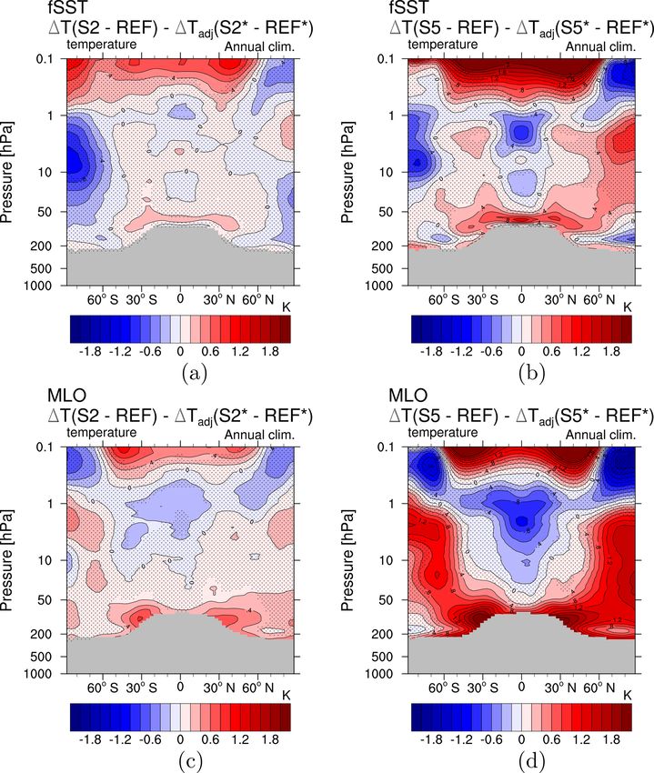
with X being either 2 or 5. A similar approach was used tropics above is shifted to the respective winter hemisphere
by, for example, Rosier and Shine (2000) and Schnadt et al. (compare Figs. S11 and S13). For S2 MLO, the warming
(2002) to distinguish between the radiative impact of trace patches in the lower stratosphere are also present in the pat-
gases and dynamical contributions to the total temperature tern of 1T̃dyn. . Apart from that, the annual mean 1T̃dyn. is
response. mostly not significant for S2 MLO. However, the pattern of
Figure 10 shows the annual mean of 1T̃dyn. for all cooling in the tropics and warming in the extratropics is indi-
four sensitivity simulations. It is mostly not significant for cated in boreal autumn (SON) and winter (DJF) for S2 MLO
S2 fSST and S5 fSST in the stratosphere, suggesting that as well.
dynamical effects play a minor role in the temperature re- We associate the main component of the 1T̃dyn. pattern of
sponse in these simulations as already indicated by Winter- the MLO experiments with the strengthening of the BDC as
stein et al. (2019). However, immediately above the tropical discussed in Sect. 3.2. Strengthened downwelling in the sub-
tropopause centred at the Equator 1T̃dyn. indicates warm- tropical and extratropical lower stratosphere results in adia-
ing for both, S2 fSST and S5 fSST. In austral winter (JJA), batic warming in this region in both hemispheres throughout
1T̃dyn. shows significant cooling in the southern polar strato- the year. These temperature changes can therefore be asso-
sphere for S2 fSST and S5 fSST. The cooling extends into ciated with the intensification of the shallow branch of the
austral spring (SON) but gradually weakens as time pro- BDC (Plumb, 2002; Birner and Bönisch, 2011). The patterns
ceeds (see Figs. S13 and S14). These temperature changes are present in S2 MLO and S5 MLO. Adiabatic cooling in the
can be associated with the strengthening of the SH strato- tropical middle and upper stratosphere as well as a respec-
spheric winter polar vortex (see Fig. S16), which leads to tive adiabatic warming in the extratropical and polar winter
enhanced isolation of air masses and stronger cooling. The stratosphere indicates the strengthening of the deep branch of
stratospheric polar vortex in boreal winter (DJF) accelerates the BDC, more pronounced in S5 MLO than in S2 MLO. The
in both fSST sensitivity simulations as well (see Fig. S15). strengthening of the BDC would be expected to result in adi-
The pattern of 1T̃dyn. for S5 MLO (Fig. 10d) displays abatic cooling directly above the tropopause from increased
a near-symmetrical behaviour around the Equator. It com- tropical upwelling. This effect seems to be masked by other
prises two warming patches in the lower stratosphere – un- processes in Fig. 10. These could be advection or mixing of
like S5 fSST not centred at the Equator but at around 30◦ S or warm air from the troposphere or increased longwave (LW)
30◦ N – as well as cooling in the tropics and warming in the radiation from the warmer troposphere and potentially more
extratropics in the middle stratosphere. The warming patches LW absorption in the lowest stratosphere. Lin et al. (2017)
in the lower stratosphere are present in all seasons, whereas found the latter effect to cause strong warming in the tropical
the pattern of cooling in the tropics and warming in the extra- tropopause layer. This radiative effect is not accounted for
Atmos. Chem. Phys., 21, 731–754, 2021 https://doi.org/10.5194/acp-21-731-2021You can also read