CisTEM, user-friendly software for single-particle image processing - Grigorieff lab
←
→
Page content transcription
If your browser does not render page correctly, please read the page content below
TOOLS AND RESOURCES

                                    cisTEM, user-friendly software for single-
                                    particle image processing
                                    Timothy Grant*, Alexis Rohou†*, Nikolaus Grigorieff*

                                    Janelia Research Campus, Howard Hughes Medical Institute, Ashburn, United
                                    States

                                    Abstract We have developed new open-source software called cisTEM (computational imaging
                                    system for transmission electron microscopy) for the processing of data for high-resolution electron
                                    cryo-microscopy and single-particle averaging. cisTEM features a graphical user interface that is
                                    used to submit jobs, monitor their progress, and display results. It implements a full processing
                                    pipeline including movie processing, image defocus determination, automatic particle picking, 2D
                                    classification, ab-initio 3D map generation from random parameters, 3D classification, and high-
                                    resolution refinement and reconstruction. Some of these steps implement newly-developed
                                    algorithms; others were adapted from previously published algorithms. The software is optimized
                                    to enable processing of typical datasets (2000 micrographs, 200 k – 300 k particles) on a high-end,
                                    CPU-based workstation in half a day or less, comparable to GPU-accelerated processing. Jobs can
                                    also be scheduled on large computer clusters using flexible run profiles that can be adapted for
                                    most computing environments. cisTEM is available for download from cistem.org.
                                    DOI: https://doi.org/10.7554/eLife.35383.001

*For correspondence:
tim@tgrant.co.uk (TG);
a.rohou@gmail.com (AR);
                                    Introduction
niko@grigorieff.org (NG)
                                    The three-dimensional (3D) visualization of biological macromolecules and their assemblies by sin-
                                    gle-particle electron cryo-microscopy (cryo-EM) has become a prominent approach in the study of
Present address: †Department        molecular mechanisms (Cheng et al., 2015; Subramaniam et al., 2016). Recent advances have been
of Structural Biology, Genentech,
                                    primarily due to the introduction of direct electron detectors (McMullan et al., 2016). With the
South San Francisco, United
                                    improved data quality, there is increasing demand for advanced computational algorithms to extract
States
                                    signal from the noisy image data and reconstruct 3D density maps from them at the highest possible
Competing interest: See             resolution. The promise of near-atomic resolution (3–4 Å), where densities can be interpreted reliably
page 22
                                    with atomic models, has been realized by many software tools and suites (Frank et al., 1996;
Funding: See page 21                Hohn et al., 2007; Lyumkis et al., 2013; Punjani et al., 2017; Scheres, 2012; Tang et al., 2007;
Received: 24 January 2018           van Heel et al., 1996). Many of these tools implement a standard set of image processing steps
Accepted: 02 March 2018             that are now routinely performed in a single particle project. These typically include movie frame
Published: 07 March 2018            alignment, contrast transfer function (CTF) determination, particle picking, two-dimensional (2D)
                                    classification, 3D reconstruction, refinement and classification, and sharpening of the final
Reviewing editor: Edward H
                                    reconstructions.
Egelman, University of Virginia,
United States
                                        We have written new software called cisTEM to implement a complete image processing pipeline
                                    for single-particle cryo-EM, including all these steps, accessible through an easy-to-use graphical
   Copyright Grant et al. This      user interface (GUI). Some of these steps implement newly-developed algorithms described below;
article is distributed under the
                                    others were adapted from previously published algorithms. cisTEM consists of a set of compiled pro-
terms of the Creative Commons
                                    grams and tools, as well as a wxWidgets-based GUI. The GUI launches programs and controls them
Attribution License, which
permits unrestricted use and        by sending specific commands and receiving results via TCP/IP sockets. Each program can also be
redistribution provided that the    run manually, in which case it solicits user input on the command line. The design of cisTEM, there-
original author and source are      fore, allows users who would like to have more control over the different processing steps to design
credited.                           their own procedures outside the GUI. To adopt this new architecture, a number of previously

Grant et al. eLife 2018;7:e35383. DOI: https://doi.org/10.7554/eLife.35383                                                          1 of 24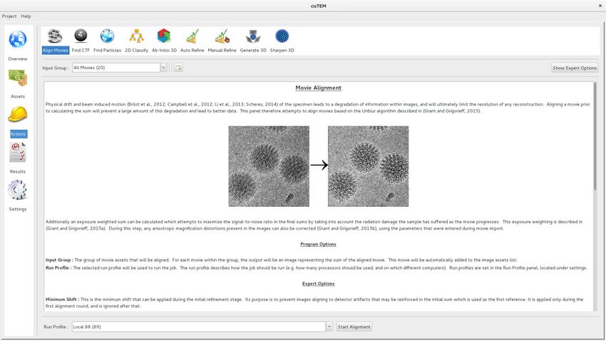
Tools and resources Structural Biology and Molecular Biophysics
existing Fortran-based programs were rewritten in C++, including Unblur and Summovie (Grant and
Grigorieff, 2015b), mag_distortion_correct (Grant and Grigorieff, 2015a), CTFFIND4 (Rohou and
Grigorieff, 2015), and Frealign (Lyumkis et al., 2013). Additionally, algorithms described previously
were added for particle picking (Sigworth, 2004), 2D classification (Scheres et al., 2005) and ab-ini-
tio 3D reconstruction (Grigorieff, 2016), sometimes with modifications to optimize their perfor-
mance. cisTEM is open-source and distributed under the Janelia Research Campus Software License
(http://license.janelia.org/license/janelia_license_1_2.html).
cisTEM currently does not support computation on graphical processing units (GPUs). Bench-
marking of a hotspot identified in the global orientational search to determine particle alignment
parameters showed that an NVIDIA K40 GPU performs approximately as well as 16 Xeon E5-2687W
CPU cores after the code was carefully optimized for the respective hardware in both cases. Since
CPU code is more easily maintained and more generally compatible with existing computer hard-
ware, the potential benefit of GPU-adapted code is primarily the lower cost of a high-end GPU com-
pared with a high-end CPU. We chose to focus on optimizing our code for CPUs.
Results
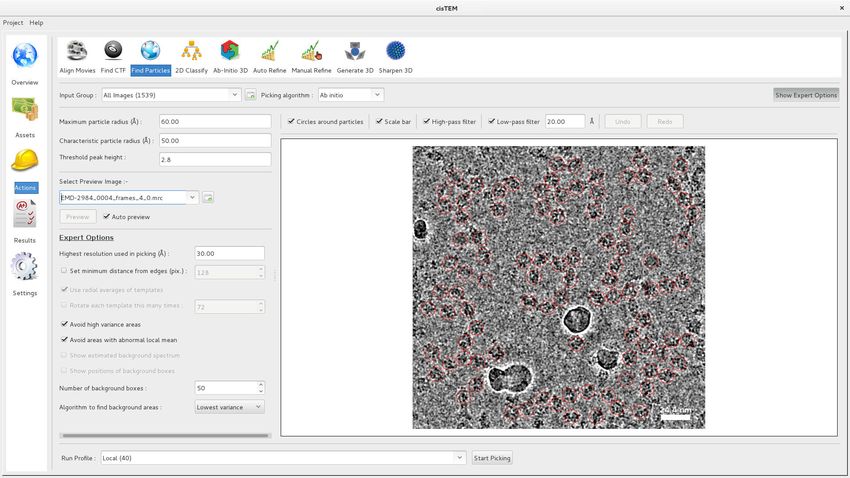
Movie alignment and CTF determination
Movie alignment and CTF determination are based on published algorithms previously implemented
in Unblur and Summovie (Grant and Grigorieff, 2015b), and CTFFIND4 (Rohou and Grigorieff,
2015), respectively, and these are therefore only briefly described here. Unblur determines the
translations of individual movie frames necessary to bring features (particles) visible in the frames
into register. Each frame is aligned against a sum of all other frames that is iteratively updated until
there is no further change in the translations. The trajectories along the x- and y-axes are smoothed
using a Savitzky–Golay filter to reduce the possibility of spurious translations. Summovie uses the
translations to calculate a final frame average with optional exposure filtering to take into account
radiation damage of protein and maximize its signal in the final average. cisTEM combines the func-
tionality of Unblur and Summovie into a single panel and exposes all relevant parameters to the user
(Figure 1). Both programs were originally written in Fortran and have been rewritten entirely in C++.
CTFFIND4 fits a calculated two-dimensional CTF to Thon rings (Thon, 1966) visible in the power
spectrum calculated from either images or movies. The fitted parameters include astigmatism and,
optionally, phase shifts generated by phase plates. When computed from movies, the Thon rings are
often more clearly visible compared to Thon rings calculated from images (Figure 2;
[Bartesaghi et al., 2014]). When selecting movies as inputs, the user can specify how many frames
should be summed to calculate power spectra. An optimal value to amplify Thon rings would be to
sum the number of frames that correspond to an exposure of about four electrons/Å2
(McMullan et al., 2015).
Since our original description of the CTFFFIND4 algorithm (Rohou and Grigorieff, 2015), several
significant changes were introduced. (1) The initial exhaustive search over defocus values can now
be performed using a one-dimensional version of the CTF (i.e. with only two parameters: defocus
and phase shift) against a radial average of the amplitude spectrum. This search is much faster than
the equivalent search over the 2D CTF parameters (i.e., four parameters: two for defocus, one for
astigmatism angle and one for phase shift) and can be expected to perform well except in cases of
very large astigmatism (Zhang, 2016). Once an initial estimate of the defocus parameter has been
obtained, it is refined by a conjugate gradient minimizer against the 2D amplitude spectrum, as
done previously. In cisTEM, the default behavior is to perform the initial search over the 1D ampli-
tude spectrum, but the user can revert to previous behavior by setting a flag in the ‘Expert Options’
of the ‘Find CTF’ Action panel. (2) If the input micrograph’s pixel size is smaller than 1.4 Å, the
resampling and clipping of its 2D amplitude spectrum will be adjusted so as to give a final spectrum
for fitting with an edge corresponding to 1/2.8 Å 1, to avoid all of the Thon rings being located
near the origin of the spectrum, where they can be very poorly sampled. (3) The computation of the
quality of fit (CCfit - 1 in [Rohou and Grigorieff, 2015]) is now computed over a moving window,
similar to (Sheth et al., 2015), rather than at intervals delimited by nodes in the CTF. (4) Following
background subtraction as described in Mindell and Grigorieff (2003), a radial, sine-edged mask is
applied to the spectrum, and this masked version is used during search and refinement of defocus,
Grant et al. eLife 2018;7:e35383. DOI: https://doi.org/10.7554/eLife.35383 2 of 24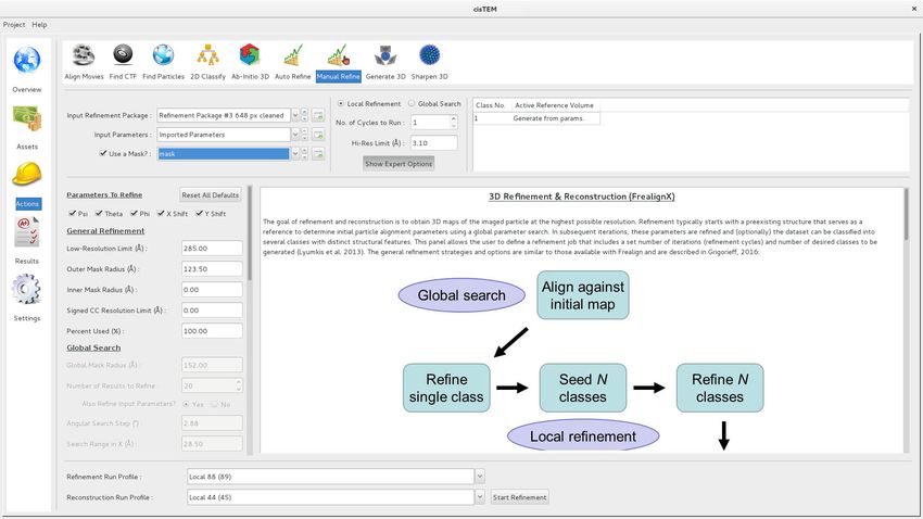
Tools and resources                                                                           Structural Biology and Molecular Biophysics

Figure 1. Movie alignment panel of the cisTEM GUI. All Action panels provide background information on the operation they control, as well as a
section with detailed explanations of all user-accessible parameters. All Action panels also have an Expert Options section that exposes additional
parameters.
DOI: https://doi.org/10.7554/eLife.35383.002

                                     astigmatism and phase shift parameters. The sine is 0.0 at the Fourier space origin, and 1.0 at a
                                     radius corresponding to 1/4 Å 1, and serves to emphasize high-resolution Thon rings, which are less
                                     susceptible to artefacts caused by imperfect background subtraction. For all outputs from the pro-
                                     gram (diagnostic image of the amplitude spectrum, 1D plots, etc.), the background-subtracted, but
                                     non-masked, version of the amplitude spectrum is used. (5) Users receive a warning if the box size of
                                     the amplitude spectrum and the estimated defocus parameters suggest that significant CTF aliasing
                                     occurred (Penczek et al., 2014).

                                     Particle picking
                                     Putative particles are found by matching to a soft-edged disk template, which is related to a convo-
                                     lution with Gaussians (Voss et al., 2009) but uses additional statistics based on an algorithm origi-
                                     nally described by Sigworth (2004). The use of a soft-edged disk template as opposed to
                                     structured templates has two main advantages. It greatly speeds up calculation, enabling picking in
                                     ‘real time’, and alleviates the problem of templates biasing the result of all subsequent processing
                                     towards those templates (Henderson, 2013; Subramaniam, 2013; van Heel, 2013). Any bias that is
                                     introduced will be towards a featureless ‘blob’ and will likely be obvious if present.
                                         Rather than fully describing the original algorithm by (Sigworth, 2004), we will emphasize here
                                     where we deviated from it. The user must specify three parameters: the radius of the template disk,
                                     the maximum radius of the particle, which sets the minimum distance between picks, and the detec-
                                     tion threshold value, given as a number of standard deviations of the (Gaussian) distribution of
                                     scores expected if no particles were present in the input micrograph. Values of 1.0 to 6.0 for this
                                     threshold generally give acceptable results. All other parameters mentioned below can usually
                                     remain set to their default values.

Grant et al. eLife 2018;7:e35383. DOI: https://doi.org/10.7554/eLife.35383                                                                       3 of 24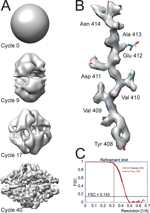
Tools and resources                                                                         Structural Biology and Molecular Biophysics

Figure 2. Thon ring pattern calculated for micrograph ‘0000’ of the high-resolution dataset of b-galactosidase (Bartesaghi et al., 2015) used to
benchmark cisTEM. The left pattern was calculated from the average of non-exposure filtered and aligned frames while the right pattern was calculated
using the original movie with 3-frame sub-averages. The pattern calculated using the movie shows significantly stronger rings compared to the other
pattern.
DOI: https://doi.org/10.7554/eLife.35383.003

                                        Prior to matched filtering, micrographs are resampled by Fourier cropping to a pixel size of 15 Å
                                    (the user can override this by changing the ‘Highest resolution used in picking’ value from its default
                                    30 Å), and then filtered with a high-pass cosine-edged aperture to remove very low-frequency den-
                                    sity ramps caused by variations in ice thickness or uneven illumination.
                                        The background noise spectrum of the micrograph is estimated by computing the average rota-
                                    tional power spectrum of 50 areas devoid of particles, and is then used to ‘whiten’ the background
                                    (shot +solvent) noise of the micrograph. Normalization, including CTF effects, and matched filtering
                                    are then performed as described (Sigworth, 2004), except using a single reference image and no
                                    principal components’ decomposition. When particles are very densely packed on micrographs, this
                                    approach can significantly over-estimate the background noise power so that users may find they
                                    have to use lower thresholds for picking. It might also be expected that under those circumstances,
                                    micrographs with much lower particle density will suffer from a higher rate of false-positive picks.
                                        One difficulty in estimating the background noise spectrum of the micrograph is to locate areas
                                    devoid of particles without a priori knowledge of their locations. Our algorithm first computes a map
                                    of the local variance and local mean in the micrograph (computed over the area defined by the maxi-
                                    mum radius given by the user [Roseman, 2004; Van Heel, 1982]) and the distribution of values of
                                    these mean and variance maps. The average radial power spectrum of the 50 areas of the micro-
                                    graph with the lowest local variance is then used as an estimate of the background noise spectrum.
                                    Optionally, the user can set a different number of areas to be used for this estimate (for example if
                                    the density of particles is very high or very low) or use areas with local variances closest to the mode
                                    of the distribution of variances, which may also be expected to be devoid of particles.
                                        Matched-filter methods are susceptible to picking high-contrast features such as contaminating
                                    ice crystals or carbon films. (Sigworth, 2004) suggests subtracting matched references from the
                                    extracted boxes and examining the remainder in order to discriminate between real particles and
                                    false positives. In the interest of performance, we decided instead to pick using a single artificial ref-
                                    erence (disk) and to forgo such subtraction approaches. To avoid picking these kinds of artifacts, the

Grant et al. eLife 2018;7:e35383. DOI: https://doi.org/10.7554/eLife.35383                                                                    4 of 24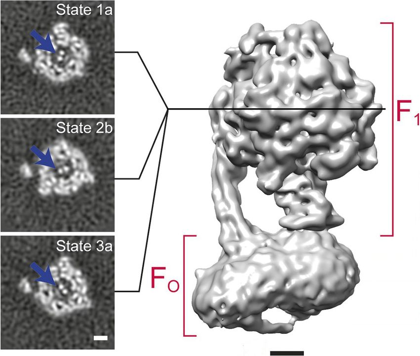
Tools and resources                                                                           Structural Biology and Molecular Biophysics

                                     user can choose to ignore areas with abnormal local variance or local mean. We find that ignoring
                                     high-variance areas often helps avoid edges of problematic objects, e.g. ice crystals or carbon foils,
                                     and that avoiding high- and low-mean areas helps avoid picking from areas within them, e.g. the car-
                                     bon foil itself or within an ice crystal (Figure 3). The thresholds used are set to Mo þ 2 FWHM for the
                                     variance and Mo  2 FWHM for the mean, where Mo is the mode (i.e. the most-commonly-occurring
                                     value) and FWHM the full width at half-maximum of the distribution of the relevant statistic. For
                                     micrographs with additional phase plate phase shifts between 0.1 and 0.9 p, where much higher con-
                                     trast is expected, the variance threshold is increased to Mo þ 8 FWHM. We have found that in favor-
                                     able cases many erroneous picks can be avoided. Remaining false-positive picks are removed later
                                     during 2D classification.
                                        Because of our emphasis on performance, our algorithm can be run nearly instantaneously on a
                                     typical ~4K image, using a single processor. In the Action panel, the user is presented with an ‘Auto
                                     preview’ mode to enable interactive adjustment of the picking parameters (Figure 3). In this mode,
                                     the micrograph is displayed with optional and adjustable low-pass and high-pass filters, and the
                                     results of picking using the currently selected parameters are overlaid on top. Changing one or
                                     more of the parameters leads to a fast re-picking of the displayed micrograph, so that the parame-
                                     ters can be optimized in real-time. Once the three main parameters have been adjusted appropri-
                                     ately, the full complement of input micrographs can be picked, usually in a few seconds or minutes.
                                        A possible disadvantage of using a single disk template exists when the particles to be picked are
                                     non-uniform in size or shape (e.g. in the case of an elongated particle). In this case, it may be
                                     expected that a single template would have difficulty in picking all the different types and views of
                                     particles present, and that in this case using a number of different templates would lead to a more

Figure 3. Particle picking panel of the cisTEM GUI. The panel shows the preview mode, which allows interactive tuning of the picking parameters for
optimal picking. The red circles overlaying the image of the sample indicate candidate particles. The picking algorithm avoids areas of high variance,
such as the ice contamination visible in the image.
DOI: https://doi.org/10.7554/eLife.35383.004

Grant et al. eLife 2018;7:e35383. DOI: https://doi.org/10.7554/eLife.35383                                                                       5 of 24
Tools and resources Structural Biology and Molecular Biophysics
accurate picking. In practice, we found that with careful optimization of the parameters, elongated
particles and particles with size variation (Figure 3) were picked adequately.
The underlying implementation of the algorithm supports multiple references as well as reference
rotation. These features may be exposed to the graphical user interface in future versions, for exam-
ple enabling the use of 2D class averages as picking templates (Scheres, 2015).
2D classification
2D classification is a relatively quick and robust way to assess the quality of a single-particle dataset.
cisTEM implements a maximum likelihood algorithm (Scheres et al., 2005) and generates fully CTF-
corrected class averages that typically display clear high-resolution detail, such as secondary struc-
ture. Integration of the likelihood function is done by evaluating the function at defined angular
steps da that are calculated according to
da ¼ R=D (1)
where R is the resolution limit of the data and D is the diameter of the particle (twice the mask radius
that is applied to the iteratively-refined class averages). cisTEM runs a user-defined number of itera-
tions n defaulting to 20. To speed up convergence, the resolution limit is adjusted as a function of
iteration cycle l (0 lTools and resources Structural Biology and Molecular Biophysics
ti ¼ 0:3maxAi;j (5)
j
where j runs over all pixels in average Ai .
3D refinement (FrealignX)
The refinement of 3D reconstructions in cisTEM uses a version of Frealign (Lyumkis et al., 2013)
that was specifically designed to work with cisTEM. Most of Frealign’s control parameters are
exposed to the user in the ‘Manual Refine’ Action panel (Figure 4). The ‘Auto Refine’ and ‘Ab-Initio’
panels also use Frealign but manage many of the parameters automatically (see below). Frealign’s
algorithm was described previously (Grigorieff, 2007; Lyumkis et al., 2013) and this section will
mostly cover important differences, including a new objective function used in the refinement, differ-
ent particle weighting used in reconstructions, optional likelihood-based blurring, as well as new
masking options.
Matched filter
To make Frealign compatible with cisTEM’s GUI, the code was completely rewritten in C++, and it
will be referred to here as Frealign v10, or FrealignX. The new version makes use of a matched filter
(McDonough and Whalen, 1995) to maximize the signal in cross correlation maps calculated
between particle images and reference projections. This requires whitening of the noise present in
the images and resolution-dependent scaling of the reference projections to match the signal in the
noise-whitened images. Both can be achieved if the spectral signal-to-noise ratio (SSNR) of the data
is known. As part of a 3D reconstruction, Frealign calculates the resolution-dependent PSSNR, the
radially averaged SSNR present in the particle images before they are affected by the CTF
Figure 4. Manual refinement panel with Expert Options exposed. Most of the parameters needed to run FrealignX can be accessed on this panel. The
panel also allows application of a 3D mask, which can be imported as a Volume Asset.
DOI: https://doi.org/10.7554/eLife.35383.005
Grant et al. eLife 2018;7:e35383. DOI: https://doi.org/10.7554/eLife.35383 7 of 24Tools and resources Structural Biology and Molecular Biophysics
(Sindelar and Grigorieff, 2012). Using PSSNR and the CTF determined for a particle, the SSNR in
the particle image can be calculated as
SNRðgÞ ¼ PSSNRðgÞ CTF 2 ðgÞ (6)
(as before, g is the 2D reciprocal space coordinate and g ¼ jgj). Here, SNR is defined as the ratio of
n~ o
the variance of the signal and the noise. The Fourier transform F Xi of the noise-whitened particle
~
image Xi can then be calculated as
n~ o F fXi gðgÞ pffiffiffiffiffiffiffiffiffiffiffiffiffiffiffiffiffiffiffiffiffiffiffi
F Xi ðgÞ ¼ qffiffiffiffiffiffiffiffiffiffiffiffiffiffiffiffiffiffiffiffiffiffiffiffiffi 1 þ SNRðgÞ (7)
jF fXi gj2r ðgÞ
where F fXi g is the Fourier transform of the original image Xi , j j is the absolute value, and jF fXi gj2r
is the radially averaged spectrum of the squared 2D Fourier transform amplitudes of image Xi . To
implement Equation (7), a particle image is first divided by its amplitude spectrum, which includes
power from both signal and noise, and then multiplied by a term that amplifies the image ampli-
tudes according to the signal strength in the image. The reference projection Ai can be matched by
calculating
n~ o F fAi gðgÞ pffiffiffiffiffiffiffiffiffiffiffiffiffiffiffi
F Ai ðgÞ ¼ qffiffiffiffiffiffiffiffiffiffiffiffiffiffiffiffiffiffiffiffiffiffiffiffiffi SNRðgÞ (8)
jF fAi gj2r ðgÞ
Equation (8) scales the variance of the signal in the reference to be proportional to the measured
signal-to-noise ratio in the noise-whitened images. The main term in the objective function OðfÞ
maximized in FrealignX is therefore given by the cross-correlation function
n~ o n ~ o
Re F R0;R3 Ai ðfÞ F R1;R3 Xi
CC ðfÞ ¼ n~ o n~ o (9a)
F R1;R3 Ai ðfÞ F R1;R3 Xi
where f is a set of parameters describing the particle view, x,y position, magnification and defocus,
Reð Þ is the real part of a complex number, k k is the Euclidean norm, i.e. the square root of the
sum of the squared pixel values, and F R1;R3 f g is the conjugate complex value of the Fourier trans-
form F R1;R3 f g. The subscripts R1 and R3 specify the low- and high-resolution limits of the Fourier
transforms included in the calculation of Equation (9a), as specified by the user. To reduce noise
overfitting, the user has the option to specify also a resolution range in which the absolute value of
the cross terms in the numerator of Equation (9a) are used (Grigorieff, 2000; Stewart and Grigor-
ieff, 2004), instead of the signed values (option ‘Signed CC Resolution Limit’ under ‘Expert Options’
in the ‘Manual Refine’ Action panel). In this case
n~ o n ~ o n~ o n ~ o
Re F R1;R2 Ai ðfÞ F R1;R2 Xi þ Re F R2;R3 Ai ðfÞ F R2;R3 Xi
CC ðfÞ ¼ n~ o n~ o (9b)
F R1;R3 Ai ðfÞ F R1;R3 Xi
where R2 is specified by the ‘Signed CC Resolution Limit.’ The objective function also includes a
term RðfjQÞ to restrain alignment parameters (Chen et al., 2009; Lyumkis et al., 2013; Sig-
worth, 2004), which currently only includes the x,y positions:
2 2 !
s2 x x y y
RðfjQÞ ¼ þ (10)
M 2s2x 2s2y
where s is the standard deviation of the noise in the particle image and Q represents a set of model
parameters including the average particle positions in a dataset, x and y , and the standard devia-
tions of the x,y positions from the average values, sx and sy , and M is the number of pixels in the
mask applied to the particle before alignment. The complete objective function is therefore
Grant et al. eLife 2018;7:e35383. DOI: https://doi.org/10.7554/eLife.35383 8 of 24Tools and resources Structural Biology and Molecular Biophysics
OðfÞ ¼ CC ðfÞ þ RðfjQÞ (11)
The maximized values determined in a refinement are converted to particle scores by multiplica-
tion with 100.
CTF refinement
FrealignX can refine the defocus assigned to each particle. Given typical imaging conditions with cur-
rent instrumentation (300 kV, direct electron detector), this may be useful when particles have a size
of about 400 kDa or larger. Depending on the quality of the sample and images, these particles may
generate sufficient signal to yield per-particle defocus values that are more accurate than the aver-
age defocus values determined for whole micrographs by CTFFIND4 (see above). Refinement is
achieved by a simple one-dimensional grid search of a defocus offset applied to both defocus values
determined in the 2D CTF fit obtained by CTFFIND4. FrealignX applies this offset to the starting val-
ues in a refinement, typically determined by CTFFIND4, and evaluates the objective function, Equa-
tion (11), for each offset. The offset yielding the maximum is then used to assign refined defocus
values. In a typical refinement, the defocus offset is searched in steps of 50 Å, in a range of ±500 Å.
In the case of b-galactosidase (see below), a single round of defocus refinement changed the defo-
cus on average by 60 Å; the RMS change was 80 Å. For this refinement, the resolution for the signed
cross terms equaled the overall refinement resolution limit (3.1 Å), i.e. no unsigned cross terms were
used. The refinement produced a marginal improvement of 0.05 Å in the Fourier Shell Correlation
(FSC) threshold of 0.143, suggesting that the defocus values determined by CTFFIND4 were already
close to optimal. In a different dataset of rotavirus double-layer particles, a single round of defocus
refinement changed the defocus on average by 160 Å; the RMS change was 220 Å. In this case, the
refinement increased the resolution from ~3.0 Å to ~2.8 Å.
Masking
FrealignX has a 3D masking function to help in the refinement of structures that contain significant
disordered regions, such as micelles in detergent-solubilized membrane proteins. To apply a 3D
mask, the user supplies a 3D volume that contains positive and negative values. cisTEM will binarize
this volume by zeroing all voxels with values less than or equal to zero, and setting all other voxels
to 1, indicating the region of the volume that is inside the mask. A soft cosine-shaped falloff of spec-
ified width (e.g. 10 Å) is then applied to soften the edge of the masked region and avoid sharp
edges when the mask is applied to a 3D reconstruction. The region of the reconstruction outside the
mask can be set to zero (simple multiplication of the mask volume), or to a low-pass filtered version
of the original density, optionally downweighted by multiplication by a scaling factor set by the user.
At the edge of the mask, the low-pass filtered density is blended with the unfiltered density inside
the mask to produce a smooth transition. Figure 5 shows the result of masking the reconstruction of
an ABC transporter associated with antigen processing (TAP, [Oldham et al., 2016]). The mask was
designed to contain only density corresponding to protein and the outside density was low-pass fil-
tered at 30 Å resolution and kept with a weight of 100% in the final masked reconstruction. The
combination of masking and low-pass filtering in this case keeps a low-pass filtered version of the
density outside the mask in the reconstruction, including the detergent micelle. Detergent micelles
can be a source of noise in the particle images because the density represents disordered material.
However, at low, 20 to 30 Å resolution, micelles generate features in the images that can help in the
alignment of the particles. In the case of TAP, this masking prevented noise overfitting in the deter-
gent micelle and helped obtain a reconstruction at 4 Å resolution (Oldham et al., 2016).
3D reconstruction
In Frealign, a 3D reconstruction Vk of class average k and containing N images is calculated as
(Lyumkis et al., 2013; Sindelar and Grigorieff, 2012)
8 P 9
N qik ^
i¼1 s2i R fi ; wik CTFi F Xi
< =
1
Vk ¼ F PN qik 2
(12)
: i¼1 2 Rðfi ; wik CTFi Þ þ 1=PSSNRk ;
si
where qik is the probability of particle i belonging to class k, si is the standard deviation of the noise
Grant et al. eLife 2018;7:e35383. DOI: https://doi.org/10.7554/eLife.35383 9 of 24Tools and resources Structural Biology and Molecular Biophysics Figure 5. 3D masking with low-pass filtering outside the mask. (A) Orthogonal sections through the 3D reconstruction of the transporter associated with antigen processing (TAP), an ABC transporter (Oldham et al., 2016). Density corresponding to the protein, as well as the detergent micelle (n- Dodecyl b-D-maltoside; highlighted with arrows), is visible. (B) Orthogonal sections through a 3D mask corresponding to the sections shown in A). The sharp edges of this mask are smoothed before the mask is applied to the map. (C) Orthogonal sections through the masked 3D reconstruction. The Figure 5 continued on next page Grant et al. eLife 2018;7:e35383. DOI: https://doi.org/10.7554/eLife.35383 10 of 24
Tools and resources                                                                                          Structural Biology and Molecular Biophysics

Figure 5 continued
regions outside the mask are low-pass filtered at 30 Å resolution to remove high-resolution noise from the disordered detergent micelle, but keeping
its low-resolution signal to help particle alignment.
DOI: https://doi.org/10.7554/eLife.35383.006

                                     in particle image i, fi are its alignment parameters, wik the score-based weights (Equation (14), see
                                     below), CTFi the CTF of the particle image, Rðfi ;  Þ the reconstruction operator merging data into a
                                     3D volume according to alignment parameters fi , PSSNR the radially averaged particle SSNR
                                     derived from the FSC between half-maps (Sindelar and Grigorieff, 2012), Xi the noise-whitened
                                     image i, and F 1 f  g the inverse Fourier transform. For the calculation of the 3D reconstructions, as
                                     well as 3D classification (see below) the particle images are not whitened according to Equation (7).
                                     Instead, they are whitened using the radially- and particle-averaged power spectrum of the back-
                                     ground around the particles:
                                                                                               F fXi gðgÞ
                                                                                  ^ i ðgÞ ¼ qffiffiffiffiffiffiffiffiffiffiffiffiffiffiffiffiffiffiffiffiffiffiffiffiffiffiffiffiffiffiffi
                                                                               F X                                                                                      (13)
                                                                                             jF fBðXi Þgj2r ðgÞ

                                     where BðXi Þ is a masked version of image Xi with the area inside a circular mask centered on the
                                     particle replaced with the average values at the edge of the mask, and scaled variance to produce
                                     an average pixel variance of 1 in the whitened image Xi . Using the procedure in Equation (13) has
                                     the advantage that whitening does not depend on the knowledge of the SSNR of the data, and
                                     reconstructions can therefore be calculated even when the SSNR is not known.

                                     Score-based weighting
                                     In previous versions of Frealign, resolution-dependent weighting was applied to the particle images
                                     during reconstruction (the Frealign parameter was called ‘PBC’, (Grigorieff, 2007)). The weighting
                                     function took the form of a B-factor dependent exponential that attenuates the image data at higher
                                     resolution. FrealignX still uses B-factor weighting but the weighting function is now derived from the
                                     particle scores (see above) as

                                                                               wðscore; gÞ ¼ e
                                                                                                       BSC
                                                                                                        4    ðscore   scoreÞg2
                                                                                                                                 :                                      (14)

                                        BSC2 converts the difference between a particle score and score2,
                                                                                                          the score average, into a B-fac-
                                     tor. Setting BSC2 to zero will turn off score-based particle weighting. Scores typically vary by about
                                     10, and values for BSC2 that produce reasonable discrimination between high-scoring and low-scor-
                                     ing particles are between 2 and 10 Å2, resulting in B-factor differences between particles of 20 to
                                     100 Å2.

                                     3D classification
                                     FrealignX uses a maximum-likelihood approach for 3D classification (Lyumkis et al., 2013). Assum-
                                     ing that all images were noise-whitened according to Equation (13), which scales the variance of
                                     each image such that the average standard deviation of the noise in a pixel is 1, the probability den-
                                     sity function (PDF) of observing image Xi , given alignment parameters fi and reconstruction Vk , is
                                     calculated as (Lyumkis et al., 2013)
                                                                                  M~         "
                                                                                                  ^i                                  2 #
                                                                                                  X          CTFi  }ðVk ; fik Þ

                                                                              1                                                       ~
                                                                                                                                      M
                                                          GðXi jfik ; Vk Þ ¼            exp                                                 gðfik jQk Þ:                (15)
                                                                             2p                                    2

                                        As before, fik are the alignment parameters (usually just Euler angles and x,y shifts) determined
                                     for image i with respect to class average k, } is the projection operator producing an aligned 2D
                                                                                                                                                           2
                                     projection of reconstruction Vk according to parameters fik , Xi                                CTFi  }ðVk ; fik Þ   ~   is the sum of
                                                                                                                                                           M
                                     the squared pixel value differences between whitened image Xi and the reference projection inside
                                                                                                                                                      ~
                                     a circular mask defining the area of the particle with user-defined diameter, M is the number of

Grant et al. eLife 2018;7:e35383. DOI: https://doi.org/10.7554/eLife.35383                                                                                          11 of 24
Tools and resources Structural Biology and Molecular Biophysics
Figure 6. 3D classification of a dataset of F1FO-ATPase, revealing different conformational states (reproduced from Figure 6A and B in Zhou et al.,
2015). Sections through the F1 domain showing the g subunit (arrows) in three different states related by 120˚ rotations are shown on the left. A surface
rendering of the map corresponding to State 1a is shown on the right. Scale bars, 25 Å.
DOI: https://doi.org/10.7554/eLife.35383.007
pixels inside this mask, and gðfik jQk Þ is a hierarchical prior describing the probability of observing
alignment parameters fik given model parameters Qk (see Equation 10). Equation (15) does not
include marginalization over alignment parameters. Marginalization could be added to improve clas-
sification when particle alignments suffer from significant errors. However, this is currently not imple-
mented in cisTEM. Given the joint probability, Equation (15), determined in a refinement, the
probability qik of particle i belonging to class k can be updated as (Lyumkis et al., 2013)
GðXi jQik ; Vk Þpk
qik ¼ PK (16)
k¼1 GðXi jQik ; Vk Þp k
where the summation in the denominator is taken over all classes and the average probabilities pk
Grant et al. eLife 2018;7:e35383. DOI: https://doi.org/10.7554/eLife.35383 12 of 24Tools and resources Structural Biology and Molecular Biophysics
for a particle to belong to class k are given by the average values of qik determined in a prior itera-
tion, calculated for the entire dataset of N particles:
N
1X
pk ¼ qik : (17)
N i¼1
An example of 3D classification is shown in Figure 6 for F1FO-ATPase, revealing different confor-
mational states of the g subunit (Zhou et al., 2015).
Focused classification
3D classification can be improved by focusing on conformationally- or compositionally-variable
regions of the map. To achieve this, a mask is applied to the particle images and reference projec-
tions, the area of which is defined as the projection of a sphere with user-specified center (within the
3D reconstruction) and radius. This 2D mask is therefore defined independently for each particle, as
~
a function of its orientation. When using focused classification, M in Equation (15) is adjusted to the
number of pixels inside the projected mask and the sum of the squared pixel value differences in
Equation (15) is limited to the area of the 2D mask. By applying the same mask to image and refer-
ence, only variability inside the masked region is used for 3D classification. Other regions of the map
are ignored, leading to a ‘focusing’ on the region of interest. The focused mask also excludes noise
contained in the particle images outside the mask and therefore improves classification results that
often depend on detecting small differences between particles and references. A typical application
of a focused mask is in the classification of ribosome complexes that may exhibit localized conforma-
tional and/or compositional variability, for example the variable conformations of an IRES
(Abeyrathne et al., 2016) or different states of tRNA accommodation (Loveland et al., 2017).
Likelihood-based blurring
In some cases, the convergence radius of refinement can be improved by blurring the reconstruction
according to a likelihood function. This procedure is similar to the maximization step in a maximum
likelihood approach (Scheres, 2012). The likelihood-blurred reconstruction is given by
PN 1 R
G Xi jfi ; Vnk 1 Rðfi ; wi CTFi Xi Þdfaxy
i¼1 s 2 f
Vnk ¼
axy
i
PN qik 2
(18)
i¼1 s2 Rðfi ; wi CTFi Þ þ 1=PSSNRk
i
where, in the case of FrealignX, faxy only includes the x,y particle positions and in-plane rotation
angle a, which are a subset of the alignment parameters fi , and Vkn 1 is the reconstruction from an
earlier refinement iteration. As before, G Xi jfi ; Vnk 1 is the probability of observing image i, given
alignment parameters fi and reconstruction Vkn 1 . Integration over these three parameters can be
efficiently implemented and, therefore, does not produce a significant additional computational
burden.
Resolution assessment
The resolution of reconstructions generated by FrealignX is assessed using the FSC criterion
(Harauz and van Heel, 1986) using the 0.143 threshold (Rosenthal and Henderson, 2003). FSC
curves in cisTEM are calculated using two reconstructions (‘half-maps’) calculated either from the
even-numbered and odd-numbered particles, or by dividing the dataset into 100 equal subsets and
using the even- and odd-numbered subsets to calculate the two reconstructions (in the cisTEM GUI,
the latter is always used). The latter method has the advantage that accidental duplication of par-
ticles in a stack is less likely to affect the FSC calculation. All particles are refined against a single ref-
erence and, therefore, the calculated FSC values may be biased towards higher values
(Grigorieff, 2000; Stewart and Grigorieff, 2004). This bias extends slightly beyond the resolution
limit imposed during refinement, by approximately 2=Dmask , where Dmask is the mask radius used to
mask the reconstructions (see above). During auto-refinement (see below), the resolution limit
imposed during refinement is carefully adjusted to stay well below the estimated resolution of the
reconstruction and the resolution estimate is therefore unbiased (Scheres and Chen, 2012). How-
ever, users have full control over all parameters during manual refinement and will have to make
Grant et al. eLife 2018;7:e35383. DOI: https://doi.org/10.7554/eLife.35383 13 of 24Tools and resources Structural Biology and Molecular Biophysics
sure that they do not bias the resolution estimate by choosing a resolution limit that is close to, or
higher than, the estimated resolution of the final reconstruction. Calculated FSC curves are
smoothed using a Savitzky–Golay cubic polynomial that reduces the noise often affecting FSC curves
at the high-resolution end.
The FSC calculated between two density maps is dependent on the amount of solvent included
inside the mask applied to the maps. A larger mask that includes more solvent background will yield
lower FSC values than a tighter mask. To obtain an accurate resolution estimate in the region of the
particle density, one possibility is to apply a tight mask that closely follows the boundary of the parti-
cle. This approach bears the risk of generating artifacts because the particle boundary is not always
well defined, especially when the particle includes disordered domains that generate weak density
in the reconstruction. The approach in Frealign avoids tight masking and instead calculates an FSC
curve using generously masked density maps, corrected for the solvent content inside the mask
(Sindelar and Grigorieff, 2012). The corrected FSC curve is referred to as Part FSC and is calculated
from the uncorrected FSCuncor as (Oldham et al., 2016)
fFSCuncor
Part FSChalf maps ¼ ; (19)
1 þ ð f 1ÞFSCuncor
where f is the ratio of mask volume to estimated particle volume. The particle volume can be esti-
3
mated from its molecular mass Mw as 0:81Da Mw (Matthews, 1968). FSC curves obtained with the gen-
erous masking and subsequent solvent correction yield resolution estimates that are very close to
those obtained with tight masking (Figure 7C). Equation (19) assumes that both maps have similar
SSNR values, as is normally the case for the two reconstructions calculated from two halves of the
dataset, indicated by the subscript half maps. If one of the maps does not contain noise from sol-
vent background, for example when calculating the FSC between a reconstruction and a map
derived from an atomic model, the solvent-corrected FSC is given as
sffiffiffiffiffiffiffiffiffiffiffiffiffiffiffiffiffiffiffiffiffiffiffiffiffiffiffiffiffiffiffiffiffiffiffiffiffiffiffi
fFSCuncor 2
Part FSCmodel map ¼ 2
: (20)
1 þ ð f 1ÞFSCuncor
Speed optimization
FrealignX has been optimized for execution on multiple CPU cores. Apart from using optimized
library functions for FFT calculation and vector multiplication (Intel Math Kernel Library), the process-
ing speed is also increased by on-the-fly cropping in real and reciprocal space of particle images and
3D reference maps. Real-space cropping reduces the interpolation accuracy in reciprocal space and
is therefore limited to global parameter searches that do not require the highest accuracy in the cal-
culation of search projections. Reciprocal-space cropping is used whenever a resolution limit is speci-
fied by the user or in an automated refinement (ab-initio 3D reconstruction and auto-refinement).
For the calculation of in-plane rotated references, reciprocal-space padding is used to increase the
image size four-fold, allowing fast nearest-neighbor resampling in real space with sufficient accuracy
to produce rotated images with high fidelity.
Ab-initio 3D reconstruction
Ab-initio reconstruction offers a convenient way to proceed from single particle images to a 3D
structure when a suitable reference is not available to initialize 3D reconstruction and refinement.
Different ab-initio methods have been described (Hohn et al., 2007; Punjani et al., 2017;
Reboul et al., 2018) and cisTEM’s implementation follows a strategy published originally by (Grigor-
ieff, 2016). It is based on the premise that iterative refinement of a reconstruction initialized with
random angular parameters is likely to converge on the correct structure if overfitting is avoided and
the refinement proceeds in small steps to reduce the chance of premature convergence onto an
incorrect structure. The procedure is implemented as part of cisTEM’s GUI and uses FrealignX to
perform the refinements and reconstructions.
After initialization with random angles, cisTEM performs a user-specified number of global align-
ment parameter searches, recalculating the reconstruction after each search and applying an auto-
matic masking procedure to it before the next global search. Similar to 2D classification (see above),
only a randomly selected subset of the data is used in each iteration and the resolution limit applied
Grant et al. eLife 2018;7:e35383. DOI: https://doi.org/10.7554/eLife.35383 14 of 24Tools and resources Structural Biology and Molecular Biophysics
during the search is increased with every iteration. The number of iterations n defaults to 40, the
starting and final resolution limits Rstart and Rfinish default to 20 Å and 8 Å, respectively, and the start-
ing and final percentage of included particles in the reconstruction, pstart and pfinish default to
2500K=N and 10; 000K=N, respectively (results larger than one are reset to 1), with K the number of
3D classes to be calculated as specified by the user, and N the number of particles in the dataset. If
symmetry is applied, N is replaced by NOsym where Osym is the number of asymmetric units present in
one particle. The resolution limit is then updated in each iteration l as in Equation (2), and the per-
centage is updated as
p ¼ pstart þ l pfinish pstart =ðn 1Þ (21)
again resetting results larger than 1 to 1. cisTEM actually performs a global search for a percentage
3p of the particle stack, that is, three times as many particles as are included in the reconstructions
for each iteration. The particles included in the reconstructions are then chosen to be those with the
highest scores as calculated by FrealignX.
The global alignment parameters are performed using the ‘general’ FrealignX procedure with the
following changes. Firstly, the PSSNR is not directly estimated from the FSC calculated at each
round. Instead, for the first three iterations, a default PSSNR is calculated based on the molecular
weight. From the fourth iteration onwards, the PSSNR is calculated from the FSC, however if the cal-
culated PSSNR is higher than the default PSSNR, the default PSSNR is taken instead. This is done in
order to avoid some of the overfitting that will occur during refinement. Secondly, during a normal
global search the top h (where h defaults to 20) results of the grid search are locally refined, and the
best locally refined result is taken. In the ab-initio procedure, however, the result of the global search
for a given particle image is taken randomly from all results that have a score which lies in the top
15% of the difference between the worst score and the best score.
During the reconstruction steps, the calculated s for each particle is reset to 1 prior to 3D recon-
struction and score weighting is disabled. This is done because the s and score values are not mean-
ingful until an approximately correct solution is obtained.
The reconstructions are automatically masked before each new refinement iteration to suppress
noise features that could otherwise be amplified in subsequent iterations. The same masking proce-
dure is also applied during auto-refinement (see below). It starts by calculating the density average
of the reconstruction and resetting all voxel values below to . This thresholded reconstruction is
then low-pass filtered at 50 Å resolution and turned into a binary mask by setting densities equal or
below a given threshold t to zero and all others to 1. The threshold is calculated as
t ¼ filtered þ 0:03 max 500 filtered (22)
where filtered is the density average of the low-pass filtered map and max 500 is the average of the
500 highest values in the filtered map. The largest contiguous volume in this binarized map is then
identified and used as a mask for the original thresholded reconstruction, such that all voxels outside
of this mask will be set to . Finally, a spherical mask, centered in the reconstruction box, is applied
by resetting all densities outside the mask to zero.
The user has the option to repeat the ab-initio procedure multiple times using the result from the
previous run as the starting map in each new run, to increase the convergence radius if necessary. In
the case of symmetric particles, the default behavior is to perform the first 2/3rds of the iterations
without applying symmetry. The non-symmetrized map is then aligned to the expected symmetry
axes and the final 1/3rd of the iterations are carried out with the symmetry applied. This default
behavior can be changed by the user such that symmetry is always applied, or is never applied.
Alignment of the model to the symmetry axes is achieved using the following process. A brute
force grid search over rotations around the x, y and z axes is set up. At each position on the grid the
3D map is rotated using the current x, y and z parameters, and then its projection along Euler angle
(0, 0, 0) is calculated. All of the symmetry-related projections are then also calculated, and for each
one a cross-correlation map is calculated using the original projection as a reference, and the peak
within this map is found. The sum of all peaks from all symmetry-related directions is taken and the
x,y,z rotation that most closely aligns the original 3D map along the symmetry axes should provide
the highest peak sum. To improve robustness, this process is repeated for two additional angles
Grant et al. eLife 2018;7:e35383. DOI: https://doi.org/10.7554/eLife.35383 15 of 24Tools and resources Structural Biology and Molecular Biophysics
( 45,–45, 45 and 15, 70,–15) that were chosen with the aim of including different-looking areas
when the map to be aligned is unusual in some way. The x,y,z rotation that results in the largest sum
of all peaks, over all three angles, is taken as the final rotation result. Shifts for this rotation are then
calculated based on the found 2D x,y shifts between the initial and symmetry-related projections,
with the z shift being set to 0 for C symmetries. The symmetry alignment is also included as a com-
mand-line program, which can be used to align a volume to the symmetry axis when the ab-initio is
carried out in C1 only, or when using a reference obtained by some other means.
Automatic refinement
Like ab-initio 3D reconstruction, auto-refinement makes use of randomly selected subsets of the
data and of an increasing resolution limit as refinement proceeds. However, unlike the ab-initio pro-
cedure, the percentage of particles pl and the resolution limit Rl used in iteration l depend on the
resolution of the reconstructions estimated in iteration l 1. When the estimated resolution
improved in the previous cycle,
pl ¼ max½pR ; pl 1 (23)
with
2
pR ¼ 8000Ke75=Rl 1 =N (24)
where K is the number of 3D classes to be calculated and N the number of particles in the dataset.
As before, if the particle has symmetry, N is replaced by NOsym where Osym is the number of asym-
metric units present in one particle. If the calculated pl exceeds 1, it is reset to 1. The resolution limit
is estimated as
R ¼ FSC0:5 2=Dmask (25)
where FSC0:5 is the point at which the FSC, unadjusted for the solvent within the mask (see above)
crosses the 0.5 threshold and Dmask is the user-specified diameter of the spherical mask applied to
the 3D reference at the beginning of each iteration, and to the half-maps used to calculate the FSC.
The term 2=Dmask accounts for correlations between the two half-maps due to the masking (see
above). When the resolution did not improve in the previous iteration,
pl ¼ 1:5pl 1 (26)
(reset to one if resulting in a value larger than 1). At least five refinement iterations are run and
refinement stops when pl reaches 1 (all particles are included) and there was no improvement in the
estimated resolution for the last three iterations.
If multiple classes are refined, the resolution limit in Equation (25) is set independently for each
class, however the highest resolution used for classification is fixed at 8 Å. At least nine iterations are
run and refinement stops when pl reaches 1, the average change in the particle occupancy in the last
cycle was 1% or less, and there was no improvement in the estimated resolution for the last three
iterations.
In a similar manner to the ab-initio procedure, s values for each particle are set to one and score
weighting is turned off. This is done until the refinement resolution is better than 7 Å, at which point
it is assumed the model is of a reasonable quality.
Map sharpening
Most single-particle reconstructions require some degree of sharpening that is usually achieved by
applying a negative B-factor to the map. cisTEM includes a map sharpening tool that allows the
application of an arbitrary B-factor. Additionally, maps can be sharpened by whitening the power
spectrum of the reconstruction beyond a user-specified resolution (the default is 8 Å). The whitening
amplifies terms at higher resolution similar to a negative B-factor but avoids the over-amplification
at the high-resolution end of the spectrum that sometimes occurs with the B-factor method due to
its exponential behavior. Whitening is applied after masking of the map, either with a hollow spheri-
cal mask of defined inner and outer radius, or with a user-defined mask supplied as a separate 3D
volume. The masking removes background noise and makes the whitening of the particle density
Grant et al. eLife 2018;7:e35383. DOI: https://doi.org/10.7554/eLife.35383 16 of 24Tools and resources Structural Biology and Molecular Biophysics
more accurate. Both methods can be combined in cisTEM, together with a resolution limit imposed
on the final reconstruction. The whitened and B-factor-sharpened map can optionally be filtered
with a figure-of-merit curve calculated using the FSC determined for the reconstruction
(Rosenthal and Henderson, 2003; Sindelar and Grigorieff, 2012).
GUI design and workflow
cisTEM’s GUI required extensive development because it is an integral part of the processing pipe-
line. GUIs have become more commonplace in cryo-EM software tools to make them more accessi-
ble to users (Conesa Mingo et al., 2018; Desfosses et al., 2014; Moriya et al., 2017;
Punjani et al., 2017; Scheres, 2012; Tang et al., 2007). Many of the interfaces are designed as so-
called wrappers of command-line driven tools, i.e. they take user input and translate it into a com-
mand line that launches the tool. Feedback to the user takes place by checking output files, which
are also the main repository of processing results, such as movie frame alignments, image defocus
measurements and particle alignment parameters. As processing strategies become more complex
and the number of users new to cryo-EM grows, the demands on the GUI increase in the quest for
obtaining the best possible results. Useful GUI functions include guided user input (so-called wiz-
ards) that adjust to specific situations, graphical presentation of relevant results, user interaction
with running processes to allow early intervention and make adjustments, tools to manipulate data
(e.g. masking), implementation of higher-level procedures that combine more primitive processing
steps to achieve specific goals, and a global searchable database that keeps track of all processing
steps and result. While some of these functions can be or have been implemented in wrapper GUIs,
the lack of control of these GUIs over the data and processes makes a reliable implementation more
difficult. For example, keeping track of results from multiple processing steps, some of them per-
haps repeated with different parameters or run many times during an iterative refinement, can
become challenging if each step produces a separate results file. Communicating with running pro-
cesses via files can be slow and is sometimes unreliable due to file system caching. Communication
via files may complicate the implementation of higher-level procedures, which rely on the parsing of
results from the more primitive processing steps.
The cisTEM GUI is more than a wrapper as it implements some of the new algorithms in the proc-
essing pipeline directly, adjusting the input of running jobs as the refinement proceeds. It enables
more complex data processing strategies by tracking all results in a single searchable database. All
processing steps are run and controlled by the GUI, which communicates with master and slave pro-
cesses through TCP/IP. cisTEM uses an SQL database, similar to Appion (Lander et al., 2009), to
store all results (except image files), offers input functions that guide the user or set appropriate
defaults, and implements more complex procedures to automate processing where possible. cis-
TEM’s design is flexible to allow execution in many different environments, including single worksta-
tions, multiple networked workstations and large computer clusters.
User input and the display of results is organized into different panels that make up cisTEM’s
GUI, each panel dedicated to specific processing steps (for examples, see Figures 1, 3 and 4). This
design guides users through a standard workflow that most single particle projects follow: movie
alignment, CTF determination, particle picking, 2D classification, 3D reconstruction, refinement and
classification, and sharpening of the final reconstructions. Three types of panels exist, dealing with
Assets, Actions and Results. Assets are mostly data that can be used in processing steps called
Actions. They include Movies, Images, Particle Positions and Volumes. One type of Asset, a Refine-
ment Package, defines the data and parameters necessary to carry out refinement of a 3D structure
(or a set of structures if 3D classification is done), it contains a particle stack, as well as information
about the sample (e.g. particle size and molecular weight) along with parameters for each particle
(e.g. orientations and defocus values). Actions comprise the above mentioned workflow steps, with
additional options for ab-initio 3D reconstruction, as well as automatic and manual 3D refinement to
enable users to obtain the best possible results from their data. The results of most of these Actions
are stored in the database and can be viewed in the related Results panels, which display relevant
data necessary to evaluate the success of each processing step. The option to sort and select results
by a number of different metrics is available in the movie alignment and CTF estimation Results pan-
els. For example images can be sorted/selected based on the CTF fit resolution (Rohou and Grigor-
ieff, 2015). Movie alignment, 3D refinement and reconstruction also produce new Image and
Volume Assets, respectively.
Grant et al. eLife 2018;7:e35383. DOI: https://doi.org/10.7554/eLife.35383 17 of 24You can also read