Measuring the state and temporal evolution of glaciers in Alaska and Yukon using synthetic-aperture-radar-derived (SAR-derived) 3D time series of ...
←
→
Page content transcription
If your browser does not render page correctly, please read the page content below
The Cryosphere, 15, 4221–4239, 2021
https://doi.org/10.5194/tc-15-4221-2021
© Author(s) 2021. This work is distributed under
the Creative Commons Attribution 4.0 License.

Measuring the state and temporal evolution of glaciers in Alaska
and Yukon using synthetic-aperture-radar-derived (SAR-derived)
3D time series of glacier surface flow
Sergey Samsonov1 , Kristy Tiampo2 , and Ryan Cassotto2
1 Canada  Centre for Mapping and Earth Observation, Natural Resources Canada, 560 Rochester Street,
Ottawa, ON K1S5K2 Canada
2 Earth Science and Observation Center, Cooperative Institute for Research in Environmental Sciences,

University of Colorado, Boulder, CO 80309 USA

Correspondence: Sergey Samsonov (sergey.samsonov@nrcan-rncan.gc.ca)

Received: 4 September 2020 – Discussion started: 27 October 2020
Revised: 27 July 2021 – Accepted: 29 July 2021 – Published: 6 September 2021

Abstract. Climate change has reduced global ice mass over         1   Introduction
the last 2 decades as enhanced warming has accelerated sur-
face melt and runoff rates. Glaciers have undergone dynamic       The magnitude and direction of glacier flow adjust in re-
processes in response to a warming climate that impacts the       sponse to the warming climate, leading to changes in sea-
surface geometry and mass distribution of glacial ice. Un-        sonal flooding and droughts, landscapes and habitats, and
til recently no single technique could consistently measure       ultimately sea level variations. Surface flow is a key vari-
the evolution of surface flow for an entire glaciated region in   able for determining glacier mass balance (Shepherd et al.,
three dimensions with high temporal and spatial resolution.       2020), ice thickness (Morlighem et al., 2011; Werder et al.,
We have improved upon earlier methods by developing a             2019), and surface mass balance (Bisset et al., 2020). Here
technique for mapping, in unprecedented detail, the temporal      we present a technique that can be used for measuring the
evolution of glaciers. Our software computes north, east, and     temporal evolution of surface flow for an entire glaciated re-
vertical flow velocity and/or displacement time series from       gion in three dimensions (3D) with high temporal and spatial
the synthetic aperture radar (SAR) ascending and descending       resolution.
range and azimuth speckle offsets. The software can handle           Modern techniques and platforms used for monitoring
large volumes of satellite data and is designed to work on        glacier flow include synthetic aperture radar (SAR) (Gold-
high-performance computers (HPCs) as well as workstations         stein et al., 1993; Mohr et al., 1998; Rignot, 2002; Joughin,
by utilizing multiple parallelization methods. We then com-       2002), the Global Navigation Satellite System (GNSS)
pute flow velocity–displacement time series for glaciers in       (van de Wal et al., 2008; Bartholomew et al., 2010), opti-
southeastern Alaska during 2016–2021 and observe seasonal         cal imagery (Berthier et al., 2005; Herman et al., 2011; De-
and interannual variations in flow velocities at Seward and       hecq et al., 2015; Fahnestock et al., 2016), and uncrewed
Malaspina glaciers as well as culminating phases of surging       aerial vehicles (Immerzeel et al., 2014). Among these, SAR
at Klutlan, Walsh, and Kluane glaciers. On a broader scale,       is the only active side-looking sensor with global coverage at
this technique can be used for reconstructing the response        high temporal and spatial resolution that can operate in any
of worldwide glaciers to the warming climate using archived       weather conditions, day or night. SAR techniques comprise
SAR data and for near-real-time monitoring of these glaciers      displacement measurements with sub-meter to meter-scale
using rapid revisit SAR data from satellites, such as Sentinel-   precision using speckle offset tracking (SPO) (Strozzi et al.,
1 (6 or 12 d revisit period) and the forthcoming NISAR mis-       2002), split-beam interferometry (or multi-aperture interfer-
sion (12 d revisit period).                                       ometry, MAI) (Bechor and Zebker, 2006; Gourmelen et al.,
                                                                  2011), and centimeter-scale differential interferometry (DIn-

Published by Copernicus Publications on behalf of the European Geosciences Union.
4222                     S. Samsonov et al.: Measuring the state and temporal evolution of glaciers in Alaska and Yukon

SAR) (Massonnet and Feigl, 1995; Rosen et al., 2000). SPO         sented in this paper), and 4D (Samsonov et al., 2021a) ve-
applies image correlation algorithms to radar data to measure     locity and/or displacement time series. Finally, the software
displacements in the satellite range and azimuth directions       is also parallelized (OpenMP, MPI), making it suitable for
using two SAR images. Since its early inception, SAR has          running on high-performance computers (HPCs) or personal
been used in glacier monitoring for estimating flow veloc-        workstations.
ities, surface flux, tidal variations, grounding line behavior,      In contrast to MSBAS-based techniques, Minchew et al.
and subglacial lake activity (Goldstein et al., 1993; Joughin     (2017) and Milillo et al. (2017) took a different approach
et al., 1995, 1998; Rignot, 1998; Shepherd et al., 2001; Gray     and inferred time-dependent 3D flow velocity by assuming a
et al., 2005; Palmer et al., 2010; Minchew et al., 2017). In      form for the temporal basis functions based on prior knowl-
this study, we use the SPO technique to produce deformation       edge of the study area. The need for prior knowledge means
maps in range and azimuth coordinates that do not require         that this method is not general, so its application is limited
phase unwrapping.                                                 to areas where the assumed basis functions should be valid.
   The SAR-derived displacements for a single epoch can           The advantage of the Minchew et al. (2017) approach is inter-
be transformed into 3D (north, east, vertical) displacements      pretability of the results, a straightforward connection of the
by either combining multiple datasets or assuming various         results to the physics of the systems being observed, and ro-
model constraints (Mohr et al., 1998; Wright et al., 2004;        bust quantification of uncertainties. A recent improvement to
Gourmelen et al., 2007; Kumar et al., 2011; Hu et al., 2014).     Minchew et al. (2017) is Riel et al. (2021), who adopted some
However, the 3D displacement time series cannot be easily         of the methods of Riel et al. (2014, 2018) and applied them to
computed due to limitations inherent in the data acquisition      remote sensing observations of glaciers. From a methodolog-
strategy. Specifically, SAR data on ascending and descending      ical perspective, this generalizes the approach of Minchew
orbits are usually acquired on different days, often with dif-    et al. (2017) and allows for a generic set of temporal ba-
ferent incidence angles and varying temporal and spatial res-     sis functions, from which a sparsity-inducing optimization
olutions and wavelengths. The multidimensional small base-        is used to identify the simplest set of basis functions that
line subset (MSBAS) methodology (Samsonov and d‘Oreye,            describe the data. The advantage there is also in the inter-
2012, 2017; Samsonov, 2019; Samsonov et al., 2020) has            pretability of the results and robust uncertainty quantifica-
been developed specifically for computing multidimensional        tion, which provides the ability to decompose the observed
displacement time series from SAR data acquired with dif-         signal into short- and long-term variations and features the
ferent acquisition parameters.                                    ability to constrain transients, secular, and periodic signals.
   Historically, three components of mean glacier velocity        However, this method still requires a priori knowledge to
were computed from DInSAR and/or range offsets by in-             provide confidence in the resulting basis functions. The tech-
troducing a surface-parallel flow (SPF) constraint. This ap-      nique we present here is complementary because it does not
proach was used for 3D mapping of Greenlandic (Joughin            rely on basis functions and provides flexibility at the expense
et al., 1998; Mohr et al., 1998) and Himalayan (Kumar et al.,     of interpretability of the results, whereas the Minchew et al.
2011) glaciers and validated by independent GNSS (Kumar           (2017) and Riel et al. (2021) techniques sacrifice flexibility
et al., 2011) measurements. In our previous work (Samsonov,       in the method for enhanced interpretability of the results.
2019), we adopted the SPF method for computing the 3D                Here we focus on dynamic changes along six land-
flow displacement time series of the Barnes Ice Cap using         terminating glaciers in southeastern Alaska during 20 Oc-
ascending and descending DInSAR data combined using the           tober 2016–21 January 2021: Agassiz, Seward, Malaspina,
MSBAS technique. However, the SPF constraint ignores sub-         Klutlan, Kluane, and Walsh glaciers. This technique can be
mergence and emergence velocities and other vertical mo-          used to analyze 3D flow velocities of glacier surfaces over
tion. In some studies, ascending and descending DInSAR            large regional scales using nearly 3 decades of archived SAR
(Gray, 2011) or range and azimuth offsets (Wang et al., 2019)     data and for near-real-time monitoring of these glaciers using
were used to compute 3D glacier velocities for a few isolated     rapid revisit SAR data.
epochs. Recently, Guo et al. (2020) developed a technique
based on MSBAS that computes 3D flow velocity time se-
ries from ascending and descending range and azimuth off-         2   Model
sets and used it to study Hispar Glacier in central Karako-
                                                                  The inversion technique described below utilizes ascending
ram. Here, we present our independently developed version
                                                                  and descending range and azimuth speckle offset products
of this algorithm, which offers several distinct advantages
                                                                  computed from SAR data using a speckle offset tracking al-
over Guo et al. (2020). First, our technique does not use
                                                                  gorithm implemented in GAMMA software (Wegmuller and
weights determined by the pixel spacing. Second, our open-
                                                                  Werner, 1997). We chose to use the speckle offsets because
source software provides additional functionalities, such as
                                                                  their computation does not require phase unwrapping, which
zeroth-, first- (implemented in Guo et al., 2020), and second-
                                                                  is not possible due to large flow velocities in our study area.
order Tikhonov regularizations. Third, the user can choose
to compute 1D, 2D, constrained 3D, unconstrained 3D (pre-

The Cryosphere, 15, 4221–4239, 2021                                                  https://doi.org/10.5194/tc-15-4221-2021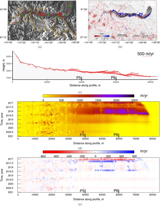
S. Samsonov et al.: Measuring the state and temporal evolution of glaciers in Alaska and Yukon 4223
greater than the number of unknowns. In the equal case, the
matrix is square and no regularization is required (but can
still be applied). In the greater case, the least square solu-
tion is found using singular value decomposition (SVD); this
scenario is common in 1D MSBAS, wherein usually there
are more interferograms than single-look complex (SLC) im-
ages. In the lesser case, as always in 2D and 3D MSBAS,
the solution is found using either the truncated SVD or the
Figure 1. Schematics of the simplified case described by Eq. (3).
Ascending and descending SAR acquisitions at time ti are marked zeroth-order Tikhonov regularization. The higher-order reg-
with black stars. Horizontal solid lines represent range and azimuth ularizations must be applied if the objective is to fill the tem-
offset maps. Vertical dashed lines divide temporal scale in time in- poral gaps due to missing data, which results in smoothing
tervals 1ti = ti+1 − ti between consecutive acquisitions. The times and the interpolation of missing values in the temporal do-
of first and last descending acquisitions (marked with blue stars) are main. We observe that the first- and second-order regular-
adjusted to match the first and last time of ascending acquisitions izations work equally well in this case, probably because of
(marked with gray stars). slowly changing velocities.
In the M × N transform matrix A with M rows and N
columns, N is equal to the number of available distinct SLC
The 3D displacement time series are computed by invert- images (with the boundary correction P – defined below) mi-
ing a set of linear equations, first solving for the north, east, nus 1 then multiplied by 3 (i.e., N = 3( K k
k=1 Nslc −1), where
and vertical flow velocities Vn,e,v for each acquisition epoch K is the total number of ascending and descending sets and
(Fialko et al., 2001; Bechor and Zebker, 2006) and then for Nslck is the number of SLC images in k set). M is equal to
cumulative 3D flow displacements Dn,e,v . the total number of range and azimuth P offset maps computed
from those SLC images (i.e., M = K k k
k=1 (Nα + Nρ ), where
ROasc
K is the total number of ascending and descending sets, Nαk
AOasc
Vn
is the number of computed azimuth offset maps, and Nρk is
A
ROdsc
Ve = (1a)
λL the number of computed range offset maps in k set).
Vv AOdsc
The regularization matrix L has the same number of
0
columns N as the transform matrix A, but its number of rows
i+1 i i
Dn,e,v = Dn,e,v + Vn,e,v 1ti (1b) depends on the regularization order. It is equal to N for the
zeroth order, N −3 for the first order, and N −6 for the second
Equation (1a) has a straightforward application: time inter- order.
val multiplied by velocity is equal to displacement. Here, in The structure of A can be deduced from a simplified ex-
matrix form, RO represents the range and AO represents the ample shown in Fig. 1 and described below. In this exam-
azimuth offsets computed from SAR data; L is the Tikhonov ple, it is assumed that the ascending set consists of three
regularization matrix multiplied by the scalar regularization SAR images acquired on t0 , t2 , and t4 , and the descend-
parameter, λ, and A is the transform matrix constructed from ing set consists of four SAR images acquired on t−1 , t1 ,
the time intervals between consecutive SAR acquisitions and t3 , and t5 . Two ascending range ROasc = {ρ0−2 asc , ρ asc } and
2−4
the range (sρ ) and azimuth (sα ) directional cosines with asc asc asc
azimuth AO = {α0−2 , α2−4 } offset products are computed
north, east, and vertical components: from three ascending SAR images, and three descending
range ROdsc = {ρ−1−1 dsc , ρ dsc , ρ dsc } and azimuth AOdsc =
1−3 3−5
sρ = {snρ , seρ , svρ } = {sin(φ) sin(θ ), − cos(φ) sin(θ ), cos(θ )} dsc dsc dsc
{α−1−1 , α1−3 , α3−5 } offset products are computed from four
sα = {snα , seα , svα } = {cos(φ), sin(φ), 0}, (2) descending SAR images (therefore, M = 2+2+3+3 = 10).
A boundary correction (shown as blue arrows in Fig. 1) is ap-
where φ is the azimuth and θ is the incidence angle. The plied to the first and last descending offset products ρ−1−1 dsc ,
azimuth is the satellite heading, measured from the north; dsc , ρ dsc , and α dsc by multiplying by (t − t )/(t − t )
α−1−1 3−5 3−5 1 0 1 −1
it discerns ascending vs. descending orbits. The incidence
and (t4 − t3 )/(t5 − t3 ) in order to adjust the temporal cover-
angle is the angle between the nadir and the look direction
age to match the ascending offset products. The boundary-
from the satellite; it is one of the acquisition parameters of dsc , α dsc ,
corrected descending offsets therefore become ρ0−1 0−1
the side-looking SAR sensor. dsc dsc
The need for regularization arises because SAR images ρ3−4 , and α3−4 . Note that the boundary correction reduces
from different tracks are acquired at different times, which the number of SLC images by two; after correction, t−1 ef-
results in more unknowns than equations, producing a rank- fectively becomes t0 , and t5 effectively becomes t4 (i.e., re-
deficient, underdetermined problem. When solving a set of ducing the total number of SLC images to five and thus
linear equations in general there can be three possible sce- N = 3(5 − 1) = 12). The first-order regularization matrix L
narios: the number of equations can be less than, equal to, or in this case has 12 columns and 9 rows.
https://doi.org/10.5194/tc-15-4221-2021 The Cryosphere, 15, 4221–4239, 2021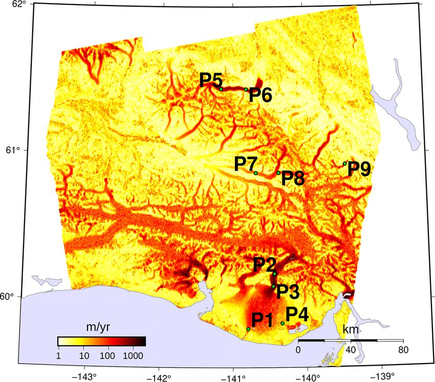
4224 S. Samsonov et al.: Measuring the state and temporal evolution of glaciers in Alaska and Yukon
Figure 2. Results of numerical simulations demonstrating the ability of this technique to reconstruct input signal in one of components.
Equations of input signals are shown in corresponding subfigure legends; t is time. Harmonic input signals are assumed. Gaussian noise with
a mean value of zero and standard deviations of 0.15 m (which is approximately 10 % of the signal) is added to subfigures in the second row.
Assuming that 1ti = ti+1 − ti in this simplified example,
Eq. (1a) becomes
asc 1t asc 1t asc 1t asc 1t asc 1t asc 1t
asc
ρ0−2
snρ seρ svρ snρ seρ svρ 0 0 0 0 0 0
0 0 0 1 1 1 asc
0 0 0 0 0 0 asc 1t
snρ 2
asc 1t
seρ 2
asc 1t
svρ 2
asc 1t
snρ 3
asc 1t
seρ 3
asc 1t
svρ 3 ρ2−4
s asc 1t asc asc asc
α asc
seα 1t0 0 snα 1t1 seα 1t1 0 0 0 0 0 0 0
nα 0 α0−2
0 asc 1t asc 1t asc 1t asc 1t
V0 asc
0 0 0 0 0 snα seα 0 snα seα 0
2 2 3 3 n 2−4
dsc dsc 1t dsc
dsc
snρ 1t0 seρ svρ 1t0 0 0 0 0 0 0 0 0 0 V 0 ρ0−1
0 e
dsc 1t dsc 1t dsc 1t dsc 1t dsc 1t dsc 1t V 0 dsc
0 0 0 snρ seρ svρ snρ seρ svρ 0 0 0 ρ1−3
1 1 1 2 2 2 v
dsc 1t dsc 1t dsc 1t V 1 dsc
0
0 0 0 0 0 0 0 0 snρ 3 seρ 3 svρ 3 n ρ3−4
s dsc 1t dsc 1t
seα 0 0 0 0 0 0 0 0 0 0 V 1 dsc
α0−1
nα 0 0 e
0 0 0 dsc 1t
snα dsc 1t
seα 0 dsc 1t
snα dsc 1t
seα 0 0 0 0 V 1 dsc
α
1 1 2 2 v = 1−3 .
(3)
0 0 0 0 0 0 0 0 0 dsc 1t
snα dsc 1t
seα 0 V 2 α dsc
3 3 n2 3−4
λ 0 0 −λ 0 0 0 0 0 0 0 0 V
e2 0
0 λ 0 0 −λ 0 0 0 0 0 0 0 V 0
0 0 λ 0 0 −λ 0 0 0 0 0 0 v3 0
Vn
0 0 0 λ 0 0 −λ 0 0 0 0 0 3
0
Ve
0 0 0 0 λ 0 0 −λ 0 0 0 0 0
Vv3
0 0 0 0 0 λ 0 0 −λ 0 0 0 0
0 0 0 0 0 0 λ 0 0 −λ 0 0
0
0 0 0 0 0 0 0 λ 0 0 −λ 0
0
0 0 0 0 0 0 0 0 λ 0 0 −λ 0
The Cryosphere, 15, 4221–4239, 2021 https://doi.org/10.5194/tc-15-4221-2021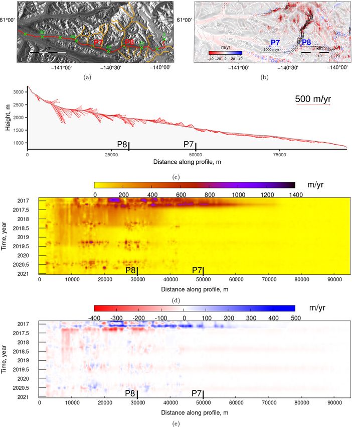
S. Samsonov et al.: Measuring the state and temporal evolution of glaciers in Alaska and Yukon                                   4225

   The 3D flow displacement time series are then computed              ity, matrix L is assumed to be a part of matrix A) in our
                     i+1 = D i
as in Eq. (1b) as Dn,e,v                i
                             n,e,v +Vn,e,v 1ti for i = {0, 1, 2, 3},   case. Thus, the total number of azimuth and range offset
assuming that the initial displacements Dn,e,v  0    are equal to      maps M equals 446, and the number of unknowns N equals
                                      0
zero. Note that in this notation Dn,e,v represents the 3D dis-         666, which corresponds to 223 SLC images after applying
placements at time t0 , while Vn,e,v0     and 1t0 are the 3D ve-       the boundary correction. The additional N − 3 = 663 rows
locities and the time interval at the time epoch t0 − t1 , thus        represent the first-order Tikhonov regularization terms. The
effectively available at time t1 . For simplicity of presenta-         singular value decomposition (SVD) algorithm from the Lin-
tion, a linear trend is computed by applying linear regres-            ear Algebra PACKage (LAPACK) library is used for invert-
sion to the derived values, calculated over the entire record,         ing this matrix for each pixel. Processing is parallelized using
to illustrate the 3D displacement time series and three linear         Open Multi-Processing (OpenMP) implementation of multi-
rate maps used for visualizing the results. Note that in the           threading. Depending on the number of cores in the process-
case of non-steady-state flow, the linear rates, which are ef-         ing unit and the number of pixels, this process can take from
fectively mean linear rates, can significantly differ from the         several hours to several days. Processing time in our case,
instantaneous flow velocities. Linear rates can potentially be         on a 44-core workstation is approximately 24 h. The Mes-
computed over a time interval of any duration (for example,            sage Passing Interface (MPI) version of the software has also
1 month or 1 year).                                                    been developed. The processing time in an MPI version is
   Tikhonov regularizations of various orders can be applied           reduced proportionally to the number of nodes.
during the inversion, resulting in temporal smoothing. The
zeroth-order regularization is effectively the constant dis-           2.1   Synthetic tests
placement constraint. The first-order regularization is effec-
tively the constant velocity constraint, and the second-order          We used synthetic tests with the actual transform matrix A,
regularization is effectively the constant acceleration con-           which is described in detail in the next section, to demon-
straint. The first- and second-order regularizations both pro-         strate the effectiveness of the proposed technique. First, we
duce good, virtually indistinguishable results. The example            reconstructed deformation components using the harmonic
above in Eq. (3) uses first-order regularization. Zeroth- and          input signal in only one of the components, which is de-
second-order regularizations are explicitly shown in Sam-              scribed in the respective legends in Fig. 2a–c. Then we added
sonov and d‘Oreye (2017) for the 2D case. The magnitude                Gaussian noise and repeated the computations (Fig. 2d–f).
of smoothing is controlled by the regularization parameter λ           The magnitude of the noise was computed as 10 % of the av-
that can be selected, for example, using the L-curve method            erage displacement between consecutive epochs. Second, we
(Hansen and O’Leary, 1993; Samsonov and d‘Oreye, 2017).                reconstructed deformation components using the complex
We used a value of 0.1 for λ selected using the L-curve                partially uncorrelated input signal: harmonic (with a differ-
method.                                                                ent period in all components) and linear input signals in the
   MSBAS methodology has been developed for computing                  horizontal components and the harmonic signals in the verti-
multidimensional time series by combining multiple DIn-                cal component. Three runs were performed with 0 %, 10 %,
SAR data acquired at different times and in various obser-             and 30 % Gaussian noise added (Fig. 3a–c). Third, we re-
vational geometries. The 2D (east and vertical) method was             constructed deformation components using the complex cor-
described in Samsonov and d‘Oreye (2012, 2017) and the                 related input signal: harmonic (with the same period in all
surface-parallel flow-constrained 3D (north, east, vertical)           components) and linear input signals in all three components.
method in Samsonov (2019) and Samsonov et al. (2020). The              Three runs were performed, again with 0 %, 10 %, and 30 %
unconstrained 3D method (i.e., without the surface-parallel            Gaussian noise added (Fig. 3d–f).
flow constraint) presented here uses both range and azimuth               Without added noise the reconstructed output signal is
measurements for computing 3D displacements. This work                 practically identical to the input signal; with added noise,
is now possible due to improved availability over large areas          the reconstructed signal still resembles the input signal very
of high-quality, high-resolution, temporally dense ascend-             well. For a quantitative assessment, we computed correlation
ing and descending SAR data and the increase in computa-               and covariance matrices between three vectors comprising
tional power that allows computing a large number of range             east, north, and vertical components of velocity at each ob-
and azimuth offset maps and inverting large matrices. Since            servation epoch. Six correlation and covariance matrices are
this method does not make any assumptions about the di-                presented in Table 2 for each of six tests shown in Fig. 3.
rection of motion, it provides the optimal solution applica-           Both matrices provide valuable information about the qual-
ble to any surface motion (e.g., glacier flow, tectonic and an-        ity of reconstruction.
thropogenic deformation). The typical size of the transform               In the covariance matrices, diagonal elements are vari-
matrix exceeds hundreds and often thousands of columns                 ances of north, east, and vertical components of the velocity.
and rows for each pixel. It is 446 × 666 (or 1109 × 666 in-            They reflect variability due to a true signal and noise. Poten-
cluding regularization terms; in the following, for simplic-           tially, an input model can be subtracted to compute variances
                                                                       due to noise; however, it is not a goal of this test. Instead,

https://doi.org/10.5194/tc-15-4221-2021                                                     The Cryosphere, 15, 4221–4239, 2021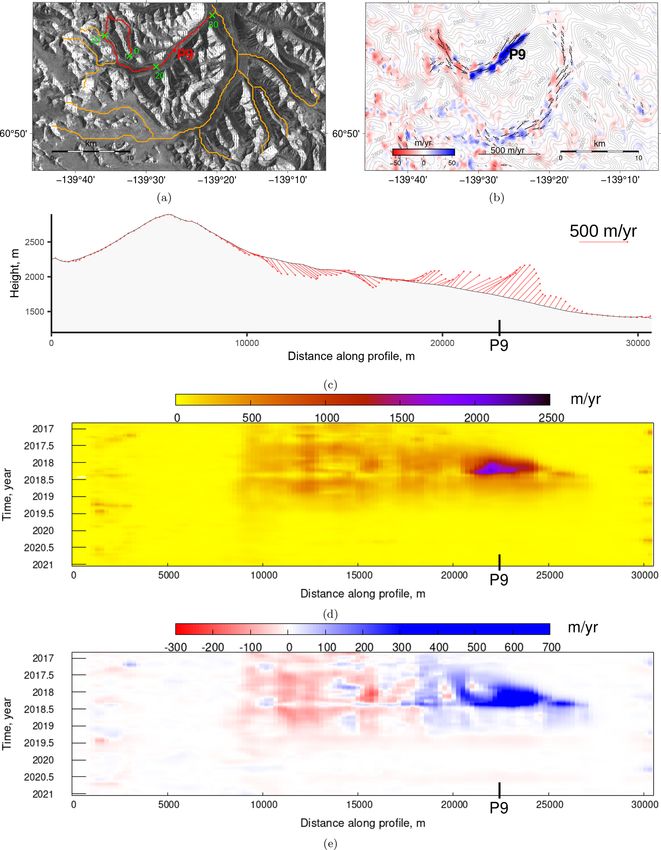
4226 S. Samsonov et al.: Measuring the state and temporal evolution of glaciers in Alaska and Yukon
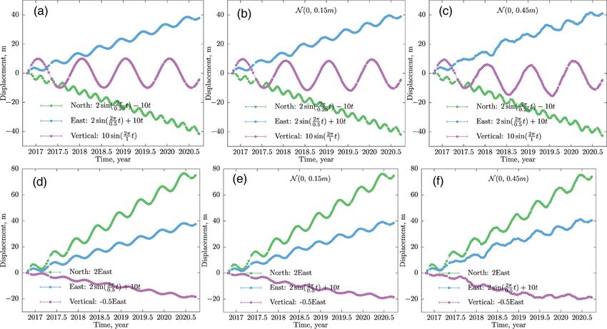
Figure 3. Results of numerical simulations demonstrating the ability of this technique to reconstruct complex uncorrelated and correlated
input signals in all three components. Equations of input signals are shown in corresponding subfigure legends; t is time. Harmonic and
linear input signals are assumed. Gaussian noise with a mean value of zero and standard deviations in the range 0.15–0.45 m (which is
approximately 10 %–30 % of the signal) is added to subfigures in the second and third columns.
Table 1. Sentinel-1 SAR data used in this study; θ is incidence and φ is azimuth angle.
Span θ◦ φ◦ Number of SLC swaths
Sentinel-1 track 123 (asc) 16 August 2016–28 January 2021 39 342 109
Sentinel-1 track 116 (dsc) 20 October 2016–21 January 2021 39 198 116
Total (after boundary correction) 20 October 2016–20 January 2021 223
we are interested in covariance (i.e., non-diagonal) terms of 3 Study area and data
the covariance matrix. They are expected to be small (com-
parable) in comparison to diagonal terms in the case of the Southeastern Alaska has experienced significant ice mass
uncorrelated (correlated) signal. In the correlation matrices, loss and retreat over the last 50 years (Arendt et al., 2009;
it is expected that non-diagonal terms should be small (close Arendt, 2011). Of the 27 000 glaciers that occupy the region,
to one) in the case of the uncorrelated (correlated) signal. the majority (99.8 %) are land-terminating (RGI Consortium,
Indeed, this pattern is clearly observed in both cases of un- 2017). Consequently, monitoring the mass balance and ice
correlated (Table 2a–c) and correlated (Table 2d–f) signals. dynamic variations of Alaska’s land-terminating glaciers is
Overall these tests indicate that the ascending–descending paramount for the future of its landscape and resultant con-
geometry is sufficient for a full reconstruction of 3D motion. tributions to sea level rise (Larsen et al., 2015). Unlike the
This can also be inferred theoretically by computing a rank plethora of ice velocity data products available for Green-
of the transform matrix in the case of one ascending and one land and Antarctica, regional studies of Alaskan glacier sur-
descending pair acquired at the same time, which would be face velocities are less abundant. The first regional map of
equal to 3. Alaskan glacier flow velocities was released in 2013 using
ALOS PALSAR data (Burgess et al., 2013). Soon after, fea-
ture tracking of Landsat optical data began to regularly map
regional surface velocities (Fahnestock et al., 2015; Gard-
ner et al., 2018, 2019). Recent studies demonstrate the im-
The Cryosphere, 15, 4221–4239, 2021 https://doi.org/10.5194/tc-15-4221-2021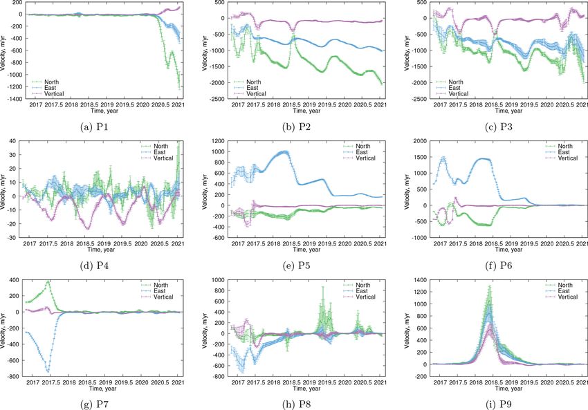
S. Samsonov et al.: Measuring the state and temporal evolution of glaciers in Alaska and Yukon 4227
Table 2. Correlation (first matrix in cell) and covariance (second matrix in cell) matrices of north, east, and vertical components of velocity
for six synthetic tests shown in Fig. 3. Labels (a)–(f) correspond to subfigures in Fig. 3. Columns are in order – north, east, vertical. Units of
covariance matrix terms are (m yr−1 )2 .
(a) (b) (c)
1.000 −0.087 −0.083 0.470 −0.023 −0.052 1.000 −0.084 −0.081 0.465 −0.022 −0.051 1.000 −0.069 −0.073 0.486 −0.021 −0.047
−0.087 1.000 −0.040 −0.023 0.143 −0.014 −0.084 1.000 −0.080 −0.022 0.151 −0.029 −0.069 1.000 −0.140 −0.021 0.201 −0.059
−0.083 −0.040 1.000 −0.052 −0.014 0.846 −0.081 −0.080 1.000 −0.051 −0.029 0.847 −0.073 −0.140 1.000 −0.047 −0.059 0.877
(d) (e) (f)
1.000 0.999 −0.997 0.581 0.287 −0.145 1.000 0.975 −0.937 0.594 0.290 −0.151 1.000 0.824 −0.681 0.653 0.297 −0.162
0.999 1.000 −0.995 0.287 0.142 −0.072 0.975 1.000 −0.923 0.290 0.149 −0.075 0.824 1.000 −0.618 0.297 0.199 −0.081
−0.997 −0.995 1.000 −0.145 −0.072 0.036 −0.937 −0.923 1.000 −0.151 −0.075 0.044 −0.681 −0.618 1.000 −0.162 −0.081 0.087
Figure 5. Spatial and temporal baselines of Sentinel-1 pairs used
in this study. Mean temporal resolution, i.e., mean temporal spac-
ing between consecutive SAR acquisitions regardless of orbit direc-
tion, computed as duration divided by the number of SAR images
(4.25 years×365/223) is about 7 d. Note that the offset between as-
cending and descending sets depends on the selection of reference
images, which is arbitrary.
portance of characterizing the temporal evolution of glacier
surface flow for understanding changes in ice dynamics in
Alaska (Waechter et al., 2015; Altena et al., 2019). However,
all regional studies of Alaskan glacier flow have so far been
limited to two dimensions, thus ignoring an important verti-
cal component of flow, which links glacier surface elevation
change and its mass balance. Here, we introduce a technique
to generate a dense record of regional Alaskan glacier surface
Figure 4. Outlines of four areas of interest (AOIs) in southeastern flow in three dimensions.
Alaska are shown in red. AOI1 covers Agassiz (AG), Malaspina We focus on studying the dynamic changes along six land-
(MG), and Seward (SG) glaciers. AOI2 covers Klutlan Glacier terminating glaciers in southeastern Alaska during 20 Oc-
(KG). AOI3 covers Walsh Glacier (WG). AOI4 covers Kluane tober 2016–21 January 2021: Agassiz, Seward, Malaspina,
Glacier. Flow lines in black and red were computed using Open Klutlan, Kluane, and Walsh glaciers (Fig. 4). The Malaspina
Global Glacier Model (OGGM) software (Maussion et al., 2019). Glacier is the world’s largest piedmont glacier covering ap-
Outlines of ascending (track 123) and descending (track 116) proximately 2200 km2 on the flat coastal foreland (Sharp,
Sentinel-1 swaths are shown in black. The background is the 30 m 1958; Muskett et al., 2003; Sauber et al., 2005) and is par-
Advanced Spaceborne Thermal Emission and Reflection Radiome- tially fed by Seward Glacier, a surge-type glacier that origi-
ter (ASTER) digital elevation model (Abrams et al., 2020). The
nates in the upper reaches of Mt. Logan (Sharp, 1951; Ford
Canada–US border is shown as a dashed black line.
et al., 2003). A mass budget deficit in the Malaspina–Seward
complex has long been recognized (Sharp, 1951). Agassiz
Glacier is another surge-type glacier that flows in an adja-
https://doi.org/10.5194/tc-15-4221-2021 The Cryosphere, 15, 4221–4239, 2021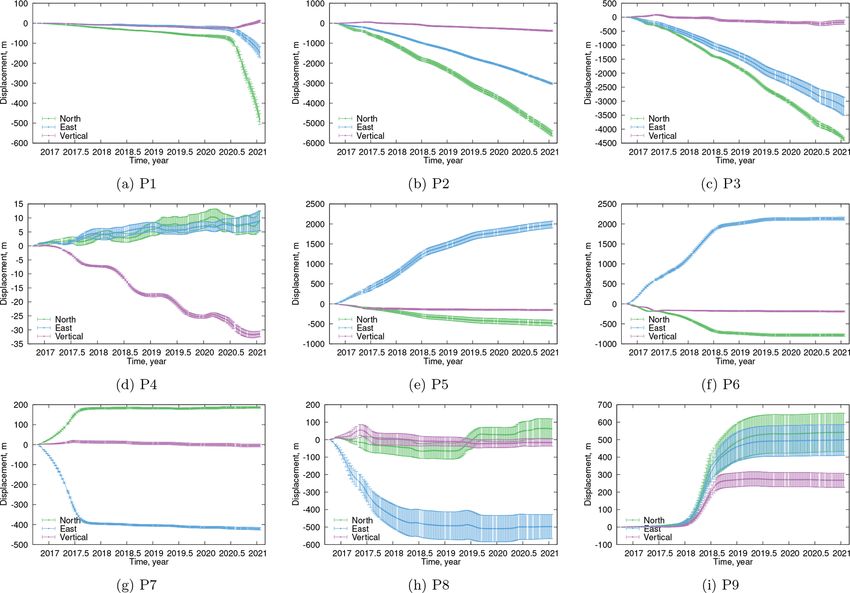
4228                      S. Samsonov et al.: Measuring the state and temporal evolution of glaciers in Alaska and Yukon

                                                                     ordinates and azimuth precision 4 times coarser than range
                                                                     precision in geocoded products. Note that the correlation
                                                                     window is not uniform, with larger weights given to the pixel
                                                                     in the center of the window. While the estimation of spatial
                                                                     resolution resulting from a nonuniform weighting of the pixel
                                                                     is beyond the scope of this study, the initial tests suggest that
                                                                     the spatial resolution is significantly better than the window
                                                                     size, which is also confirmed by the developers of GAMMA
                                                                     software (GAMMA Remote Sensing, personal communica-
                                                                     tion, 20 January 2021). Offsets were spatially filtered using a
                                                                     Gaussian filter with a 1.3 km (6-sigma) filter width, geocoded
                                                                     using the TerraSAR-X 90 m digital elevation model (DEM)
                                                                     and resampled to a common grid with a ground spacing of
                                                                     200 m. Using Gaussian weights for filtering proved to be par-
                                                                     ticularly beneficial as the filter produced satisfactory results
                                                                     for small and large glaciers. Filter width was chosen exper-
                                                                     imentally for our study but may be suboptimal in other re-
                                                                     gions.

Figure 6. Magnitude of mean 3D flow velocities plotted using loga-
rithmic scale. For regions P1–P4 at Malaspina and Seward glaciers,   4   Results
P5–P6 at Klutlan Glacier, P7–P8 at Walsh Glacier, and P9 at Kluane
Glacier time series are provided in Figs. 11 and 12.                 The magnitude of the mean 3D linear flow velocities plot-
                                                                     ted for the entire region using a logarithmic scale is shown
                                                                     in Fig. 6. An in-depth analysis was further performed for
                                                                     four small areas of interest (AOI1, AOI2, AOI3, and AOI4
cent sinuous valley northwest of the Malaspina–Seward com-
                                                                     in Fig. 4) shown in detail in Figs. 7–10. The flow lines in
plex (Muskett et al., 2003; Sauber et al., 2005). The Klutlan
                                                                     Fig. 4 were computed using the Open Global Glacier Model
Glacier is an 82 km long surge-type valley glacier located at
                                                                     (OGGM) software (Maussion et al., 2019), and the central
elevations between 1300 and 2100 m; it has surged repeat-
                                                                     flow lines were chosen for in-depth analysis. Note that these
edly over the last few hundred years (Wright, 1980; Driscoll,
                                                                     flow lines are approximated to the actual glacier flow pattern.
1980). A surge at Kluane Glacier in the eastern St. Elias
                                                                     They are, however, computed in a consistent and repeatable
Mountains during 2017/18 was previously reported in Main
                                                                     way. In addition, time series sampled from 5×5 pixel regions
et al. (2019). Walsh Glacier is a 90 km long surge-type valley
                                                                     along Malaspina and Seward glaciers (P1–P4), the Klutlan
glacier located at a higher elevation of about 1500–3000. It is
                                                                     Glacier (P5–P6), Walsh Glacier (P7–P8), and Kluane Glacier
fed by two major branches, one from the north and one from
                                                                     (P9) are provided in Figs. 11 and 12.
the east, and it converges with the Logan Glacier downstream
                                                                        For each AOI, the SAR backscatter intensity images show
(Fu and Zhou, 2020).
                                                                     the six glaciers in detail: Agassiz, Malaspina, and Seward
   In this study, we used 218 ascending (track 123) and
                                                                     (AG, MG, and SG; Fig. 7a), Klutlan (KtG; Fig. 8a), Walsh
232 descending (track 116) Sentinel-1 interferometric wide
                                                                     (WG; Fig. 9a), and Kluane (KnG; Fig. 10a) glaciers. For
(IW) single-look complex (SLC) images with 2.3 m (range)
                                                                     five of these glaciers (excluding the Agassiz Glacier) veloci-
×14.9 m (azimuth) spatial resolution from the NASA Dis-
                                                                     ties are sampled along flow lines with 20 km markers shown.
tributed Active Archive Center (DAAC) operated by the
                                                                     Mean flow velocities are shown in Figs. 7b, 8b, 9b, and 10b;
Alaska Satellite Facility (ASF) (Table 1). Two ascend-
                                                                     horizontal flow velocities are shown as vectors and vertical
ing and two descending frames along the azimuth direc-
                                                                     flow velocities are color-coded, with red representing down-
tions were concatenated for each, resulting in 109 and 116
                                                                     ward motion. For aesthetic purposes, horizontal flow vectors
swaths, respectively. Ascending and descending sets were
                                                                     are resampled to a coarser resolution. The fastest horizontal
processed individually using GAMMA software (Wegmuller
                                                                     flow velocity exceeds 1000 m yr−1 , and the fastest vertical
and Werner, 1997) that produced range and azimuth off-
                                                                     flow velocity exceeds 200 m yr−1 . Overall, Seward Glacier
sets for consecutive pairs (Fig. 5). To compute offsets, we
                                                                     experiences the fastest motion and Malaspina Glacier expe-
used a 64 × 16 pixel sampling interval (or approximately
                                                                     riences the slowest motion (Fig. 7b); vertical flow is predom-
200×200 m) and a square 128×128 pixel (or approximately
                                                                     inately downward along both glaciers. In contrast, vertical
400×1600 m) correlation window. Such a large window was
                                                                     flow along the Klutlan (Fig. 8b), Walsh (Fig. 9b), and Klu-
required to obtain a distinct, statistically significant peak of
                                                                     ane (Fig. 10b) glaciers changes direction a number of times.
the 2D cross-correlation function; its square shape produced
similar precision in range and azimuth directions in radar co-

The Cryosphere, 15, 4221–4239, 2021                                                      https://doi.org/10.5194/tc-15-4221-2021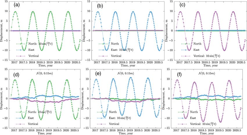
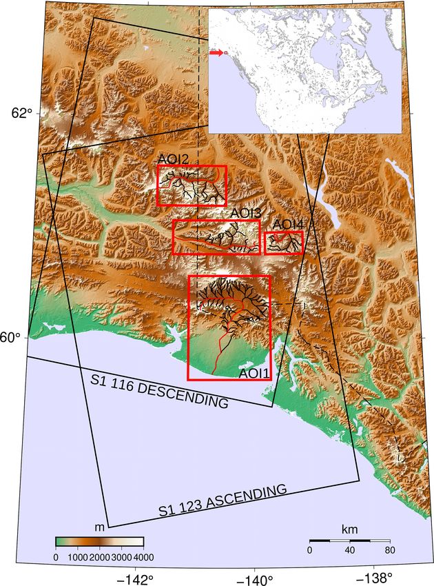
S. Samsonov et al.: Measuring the state and temporal evolution of glaciers in Alaska and Yukon                                            4229

Figure 7. (a) Sentinel-1 SAR intensity image acquired on 22 December 2019 (in YYYYMMDD format) over AOI1 that covers Agassiz
(AG), Malaspina (MG), and Seward (SG) glaciers. Flow lines are in orange and red. Markers in green show the distance in kilometers along
the selected red flow line. (b) Time-averaged 3D flow velocities: horizontal velocity is shown as a (coarse-resolution) vector map, and vertical
velocity is color-coded. Surface topographic contour lines derived from the TerraSAR-x 90 m DEM with intervals of 100 m are shown in
gray. Flow displacement time series for regions P1–P4 are plotted in Fig. 11. (c) Time-averaged 3D flow velocities and glacier height along
the red flow line. (d) Temporal evolution of horizontal flow velocity magnitude along the red flow line. (e) Temporal evolution of vertical
flow velocity along the red flow line.

https://doi.org/10.5194/tc-15-4221-2021                                                           The Cryosphere, 15, 4221–4239, 2021
4230                       S. Samsonov et al.: Measuring the state and temporal evolution of glaciers in Alaska and Yukon

Figure 8. (a) Sentinel-1 SAR intensity image acquired on 22 December 2019 over AOI2 that covers Klutlan Glacier (KtG). Flow lines are
in orange and red. Markers in green show the distance in kilometers along the selected red flow line. (b) Time-averaged 3D flow velocities:
horizontal velocity is shown as a (coarse-resolution) vector map, and vertical velocity is color-coded. Surface topographic contour lines
derived from the TerraSAR-x 90 m DEM with intervals of 100 m are shown in gray. Flow displacement time series for regions P5–P6 are
plotted in Fig. 11. (c) Time-averaged 3D flow velocities and glacier height along the red flow line. (d) Temporal evolution of horizontal flow
velocity magnitude along the red flow line. (e) Temporal evolution of vertical flow velocity along the red flow line.

The Cryosphere, 15, 4221–4239, 2021                                                            https://doi.org/10.5194/tc-15-4221-2021
S. Samsonov et al.: Measuring the state and temporal evolution of glaciers in Alaska and Yukon                                          4231

Figure 9. (a) Sentinel-1 SAR intensity image acquired on 22 December 2019 over AOI3 that covers Walsh Glacier (WG). Flow lines are
in orange and red. Markers in green show the distance in kilometers along the selected red flow line. (b) Time-averaged 3D flow velocities:
horizontal velocity is shown as a (coarse-resolution) vector map, and vertical velocity is color-coded. Surface topographic contour lines
derived from the TerraSAR-x 90 m DEM with intervals of 100 m are shown in gray. Flow displacement time series for regions P7–P8 are
plotted in Fig. 11. (c) Time-averaged 3D flow velocities and glacier height along the red flow line. (d) Temporal evolution of horizontal flow
velocity magnitude along the red flow line. (e) Temporal evolution of vertical flow velocity along the red flow line.

   The direction and magnitude of the mean linear flow ve-               in the Supplement. Note that the vertical axis (surface eleva-
locities sampled along central flow lines from Malaspina and             tion) and horizontal axis (distance along profile) are scaled
Seward, Klutlan, Walsh, and Kluane glaciers are shown in                 differently, producing significant but equal angular distortion
Figs. 7c, 8c, 9c, and 10c as vectors with tails that start at the        in the flow velocities and topographic slopes. The mean lin-
surface elevation of each glacier. Animations of these flow              ear flow velocities provide insight into the direction and mag-
velocities as time series along these profiles are also provided         nitude of mean velocities calculated over a specific interval

https://doi.org/10.5194/tc-15-4221-2021                                                          The Cryosphere, 15, 4221–4239, 2021
4232                       S. Samsonov et al.: Measuring the state and temporal evolution of glaciers in Alaska and Yukon

Figure 10. (a) Sentinel-1 SAR intensity image acquired on 22 December 2019 over AOI4 that covers Kluane Glacier (KnG). Flow lines are
in orange and red. Markers in green show the distance in kilometers along the selected red flow line. (b) Time-averaged 3D flow velocities:
horizontal velocity is shown as a (coarse-resolution) vector map, and vertical velocity is color-coded. Surface topographic contour lines
derived from the TerraSAR-x 90 m DEM with intervals of 100 m are shown in gray. Flow displacement time series for region P9 are plotted
in Fig. 11. (c) Time-averaged 3D flow velocities and glacier height along the red flow line. (d) Temporal evolution of horizontal flow velocity
magnitude along the red flow line. (e) Temporal evolution of vertical flow velocity along the red flow line.

The Cryosphere, 15, 4221–4239, 2021                                                            https://doi.org/10.5194/tc-15-4221-2021
S. Samsonov et al.: Measuring the state and temporal evolution of glaciers in Alaska and Yukon                                4233

Figure 11. 3D flow displacement time series for regions P1–P9, the locations of which are shown in Figs. 6–10.

(e.g., the Sentinel-1 record); however, these values can vary          P4. An abrupt change in a flow regime occurred at P1 at the
over time. This is evident in the temporal evolution of the            end of June 2020. Since then, the flow velocity at P1 has
horizontal velocity magnitude and vertical velocity sampled            remained elevated in comparison to the values observed in
along these profiles for the Seward and Malaspina glaciers             prior years. This many-fold velocity increase can also be ob-
(Fig. 7d and e), the Klutlan Glacier (Fig. 8d and e), the Walsh        served in Fig. 7d and e along the latter part of the profile.
Glacier (Fig. 9d and e), and the Kluane Glacier (Fig. 10d and          Horizontal and vertical flow velocities in these regions are
e). Flow along the lower reaches of the Malaspina Glacier              only a few meters per year, with a seasonal signal evident at
varies seasonally, although the seasonal acceleration was de-          P4 in the vertical component. Such seasonal signals are ob-
layed in 2020 and was higher in magnitude. Seasonal flow               served at most low-elevation glaciers. Regions P2 and P3 are
along the Klutlan, Walsh, and Kluane glaciers is far less pro-         located at elevations of about 1000 and 700 m. At these lo-
nounced; however, each shows an episodic shift in a flow that          cations, horizontal flow dominates flow displacement, while
occurred around mid-2018, mid-2017, and mid-2018, respec-              vertical flow displacement is minimal. The southwest direc-
tively.                                                                tion of flow is persistent at both locations. Flow velocities
   Examples of 3D flow displacement and velocity time se-              along the main branch of the Agassiz Glacier (not shown) are
ries for the 5 × 5 pixel regions P1–P9 are shown in Figs. 11           very similar to the flow velocities along the Seward Glacier
and 12. Similar time series can be easily produced for any             but of a lesser magnitude.
colored pixel in Fig. 6; the locations selected were chosen to            Regions P5 and P6 are located on Klutlan Glacier at ele-
demonstrate diverse ice dynamic observations possible with             vations of about 1900 and 1500 m, respectively. The overall
the MSBAS-3D method. Regions P1 and P4 are located on                  vertical flow is slightly downward in these regions, but hor-
the lower lobes of the Malaspina Glacier at an elevation of            izontal and vertical components both show significant vari-
about 200 m a.s.l. The displacement time series show that              ability over time. Regions P7 and P8 are located on Walsh
flow is predominately west-southwest at P1 and northeast at            Glacier at an elevation of about 1700 and 2000 m, respec-

https://doi.org/10.5194/tc-15-4221-2021                                                       The Cryosphere, 15, 4221–4239, 2021
4234                      S. Samsonov et al.: Measuring the state and temporal evolution of glaciers in Alaska and Yukon

Figure 12. 3D flow velocity time series for regions P1–P9, the locations of which are shown in Figs. 6–10.

tively. At P7, northwest upward displacement is observed un-            interferometry (MAI) (Bechor and Zebker, 2006) measure-
til July 2017 when a gradual reduction occurred. Region P9              ments. For high-resolution SAR data, the precision of the
is located on Kluane Glacier at an elevation of about 1700 m.           SPO technique approaches that of DInSAR. In addition to
Here, southeast and upward displacement is observed during              glaciers, this technique can be used to study other geophys-
2018 when a gradual reduction occurred. Error bars through-             ical processes (e.g., landslides, sea–river–lake ice drift) if
out Figs. 11 and 12 show measurement variability within the             their motion exceeds the sensitivity of SPO and/or MAI tech-
5×5 pixel region rather than precision, though the two quan-            niques.
tities are likely related.                                                 The reported precision of the individual offset maps com-
                                                                        puted using the SPO technique is 1/10–1/30 of the SAR
                                                                        pixel size (Strozzi et al., 2002). An average precision of
5   Discussion                                                          our speckle offset product computed over a typical inter-
                                                                        val of 12 d (i.e., Sentinel-1 repeat period) is about 1 m (or
The technique presented in this study is a viable solution for          30 m yr−1 ) in range and 4 m (or 120 m yr−1 ) in azimuth. Our
computing 3D flow displacement time series from ascend-                 precision is lower than reported in Strozzi et al. (2002) be-
ing and descending range and azimuth SAR measurements.                  cause we intentionally interpret the motion outside glaciers
Synthetic tests (Figs. 2 and 3) suggest that the precision of           (e.g., irregular snowdrift, landslides) as noise. However,
the inversion largely depends on the precision of input data            for computing the mean linear velocity the length of the
and is not limited by the Sentinel-1 suboptimal acquisition             time series is more important than the precision of indi-
geometry (i.e., nonorthogonal orbits). Range offsets can be             vidual measurements. Standard deviations of the mean lin-
substituted or complemented with DInSAR measurements                    ear velocities averaged over the entire region are 0.7, 0.3,
since both measure the same quantity; similarly, azimuth off-           and 0.2 m yr−1 (while the maximum values are 21, 18, and
sets can be substituted or complemented by multiple-aperture            7 m yr−1 , these higher values would be due to seasonal vari-

The Cryosphere, 15, 4221–4239, 2021                                                          https://doi.org/10.5194/tc-15-4221-2021
S. Samsonov et al.: Measuring the state and temporal evolution of glaciers in Alaska and Yukon 4235 ations and changes in surge activity) for northward, east- early winter scenes. One final discrepancy can be attributed ward, and vertical components, respectively. This is some- to the differences in processing parameters, such as corre- what analogous to the precision of GNSS-derived deforma- lation window and filter shape and strength. Significant fil- tion rates, which largely depend on the length of time series tering is required in our processing because, for time series rather than the precision of individual GNSS measurements. analysis, every single range and azimuth offset map must be The best approach for estimating the absolute measurement defined at every pixel, which can be only achieved by using a accuracy, of course, is comparing these remote sensing mea- large correlation window followed by strong filtering. Preser- surements with ground-based measurements (Gudmundsson vation of spatial coverage in every single range and azimuth and Bauder, 1999), which unfortunately are not available for offset map forces us to select pixels with a moderate signal- this region and this period. SAR measures glacier motion at to-noise ratio (SNR), which would not have been selected if a certain depth rather than at the surface. Previous studies for we wanted to compute only the mean velocity. Our software this region suggest that the C-band SAR penetrates ∼ 4 m can potentially handle missing values in data by interpolating into the glacier’s firn layer in dry conditions (Rignot et al., in the time domain (using first- and second-order regulariza- 2001). The standard deviation and coefficient of determina- tions), but here we have chosen not to introduce interpolation tion for each component of velocity and each pixel are pro- bias and instead lowered the SNR. Overall, in addition to pro- vided in the Supplement. viding the three components of flow velocity at a higher and One of the practical computational challenges of the SPO more consistent temporal resolution, our study demonstrates technique is the selection of pixels, the offsets of which are that deviations from the mean flow velocity can be very sig- computed with high confidence. After multiple tests, we de- nificant. Although the time series in Fig. 11 resemble GNSS- termined that the SNR function works very well for this pur- derived displacements, it is important to remember that these pose but only when the search window is large. However, Eulerian measurements represent the cumulative displace- such a large window applied to the medium-resolution SAR ment at any one pixel over time. Hence, to emphasize this data limits the spatial resolution of the results. It is possible difference, we use the flow displacement terminology. Note to use high-resolution SAR data and the 128×28 pixel search also that the vertical velocities do not represent rates of ele- window to overcome this limitation and achieve a high spa- vation change but evolving submergence and emergence ve- tial resolution of results; however, such SAR data are not yet locities indicative of broader (and faster) changes in dynamic readily available on a global scale. The utilization of high- configuration than previously understood. resolution SAR data also allows for the use of a spatial filter The overall direction of vertical flow is down along al- with a large window size in terms of pixels. most the entire length of the Seward and Malaspina glaciers We compared the magnitude of mean linear horizontal (Fig. 7). The downward flow is expected in the upper reaches flow velocities along the four profiles with the results pre- of accumulation zones because of firn compaction and in ar- sented in Gardner et al. (2019). There, surface velocities are eas with steeply dipping surfaces due to sloping bed topog- derived from Landsat 4, 5, 7, and 8 imagery over the pe- raphy; however, downward flow, with the slope steeper than riod from 1985 to 2018 using the autoRIFT feature-tracking surface topography in the lower ablation zone, is of partic- processing chain described in Gardner et al. (2018). We ular interest. In general, the accumulation of snow and ice used the horizontal velocities computed during 2017, 2018, in high elevations produces a net mass gain that replenishes and the entire 2018–present period; these results are shown ice lost through ablation processes along the lower glacier. in the Supplement. The velocities computed over the 2017 In a steady state, these processes balance each other and lead and 2018 periods (Figs. S7–S14 in the Supplement) are to submergent flow in the accumulation zone and emergent in reasonable agreement. When we compare entire datasets flow in the ablation zone; thus, ice mass lost through melt (Figs. S15–S18 in the Supplement) they still show some in the ablation zone is replenished by ice that emerges from agreement. Statistical parameters, such as correlation coef- the depths of ice columns to the glacier surface to main- ficients and room mean square errors (RMSEs), are provided tain a consistent surface elevation (Hooke, 2019). The pre- in the figure captions. We observe that in areas experienc- dominately downward flow of ice observed throughout the ing nearly constant flow velocity, for example at Seward and Malaspina Glacier’s massive lobe (Figs. 7b, c, e, and 12d) Malaspina glaciers, both datasets show close results with a indicates that ablation rates have exceeded emergence veloc- correlation of 0.93 and RMSE of 269 m yr−1 . At Klutlan, ities during our 4-year study period, implying that the glacier Walsh, and Kluane glaciers, SAR-derived velocities are af- is still adjusting to climatic warming. Indeed, the Seward, fected by the surges, which are not reflected in Gardner et al. Malaspina, and Agassiz glaciers are not in a steady state (2019), resulting in a lower correlation (0.43–0.80) and a (Muskett et al., 2003; Larsen et al., 2015). Seasonal vari- larger RMSE (80–266 m yr−1 ) in comparison to the average ability is observed along the Seward and Malaspina glaciers velocity at those glaciers. Furthermore, the Landsat record (Figs. 7d, e and 12b, c, d). The fastest horizontal motion oc- will be temporally biased towards cloud-free images and pe- curs during late spring–early summer and the slowest in late riods when sufficient sunlight is available to obtain optical summer–early fall, consistent with other glaciers in the re- imagery, thus eliminating a significant portion of late fall and gion (Abe and Furuya, 2015; Vijay and Braun, 2017; Ender- https://doi.org/10.5194/tc-15-4221-2021 The Cryosphere, 15, 4221–4239, 2021
4236                      S. Samsonov et al.: Measuring the state and temporal evolution of glaciers in Alaska and Yukon

lin et al., 2018). The fastest vertical motion is observed in the   able satellite SAR records. The horizontal components can
middle of summer. An animation provided with the Supple-            be resolved to study flow variations over time and, if inte-
ment clearly shows seasonality in flow rates over the entire        grated along a profile that is perpendicular to flow, ice flux.
complex. Seasonal variability at P1 is obstructed by a many-        The vertical component can be used to assess changes in ver-
fold increase in velocity observed in the second half of 2020       tical ice flux or changes in surface slope over time, which is
that persists at the time of this study.                            useful for studying glacier surge dynamics or variations in
   Velocities along Klutlan Glacier vary in more complex            driving stress as a glacier dynamically adjusts to a changing
ways, with multiple zones of upward and downward flow               climate. The software is freely available to the research com-
observed (Fig. 8). This surge-type glacier (RGI Consortium,         munity.
2017) has a 30- to 60-year surge cycle (Meier and Post, 1969;
Wright, 1980; Driscoll, 1980). Altena et al. (2019) used op-
tical satellite data to show that its most recent surge initi-      Code and data availability. The range and azimuth offsets com-
ated in 2014 and continued through 2017. The surge started          puted from Sentinel-1 data as well as all derived products and pro-
mid-glacier and had two propagating fronts: a dominant              cessing software used in this study can be downloaded from Mende-
surge front that propagated downglacier and a secondary sub-        ley Data at https://doi.org/10.17632/zf67rsgydv.1 (Samsonov et al.,
                                                                    2021b).
dued front that propagated upglacier. Our SAR-based record
shows that surge activity terminated in mid-2018. The time
series at P5 and P6 (Figs. 11e, f and 12e, f) show complex
                                                                    Video supplement. The animations of flow velocities for stud-
flow dynamics in both the horizontal and vertical compo-            ied glaciers (files movie_malaspina.gif, movie_klutlan.gif,
nents.                                                              movie_walsh.gif, movie_kluane.gif) are provided. Comparisons
   The Walsh Glacier is another surge-type glacier with re-         between the magnitude of mean linear horizontal flow velocities
cent surge activity. Using optical Landsat data, Fu and Zhou        along the four profiles with the results presented in Gardner et al.
(2020) showed that the latest surge initiated before 2015           (2019) are also provided.
(Fig. 9). Our SAR-based observations show residual surge
activity continued into 2017 and abruptly ended in mid-2017
(Fig. 9d). The time series at P8 (Figs. 11h and 12h) show that      Supplement. The supplement related to this article is available on-
regular increases in flow velocity during summer, while at P7       line at: https://doi.org/10.5194/tc-15-4221-2021-supplement.
these seasonal increases are less pronounced (Figs. 11g and
12g). The surge at P7 during 2017 is a dominant signal.
   A surge of the Kluane Glacier has previously been de-            Author contributions. SeS was responsible for conceptualization,
tected using RADARSAT-2 SAR measurements (Main et al.,              data curation, formal analysis, investigation, methodology, project
2019). It occurred during 2018 in a secondary valley of the         administration, resources, software, visualization, and writing (orig-
                                                                    inal draft; review and editing). KT was responsible for investiga-
glacier (Fig. 10). The entire surge cycle is captured by our
                                                                    tion, formal analysis, methodology, and writing (review and edit-
time series (Figs. 11i and 12i). Such a complex flow pattern        ing). RC was responsible for investigation, formal analysis, method-
can only be derived from side-looking SAR measurements              ology, and writing (review and editing).
that capture horizontal and vertical components of motion.
   These six in-depth-analyzed glaciers were selected from
the regional results shown in Fig. 6. Other glaciers in this        Competing interests. The authors declare that they have no conflict
region may have also experienced surges or other interesting        of interest.
behaviors. The entire dataset, which includes instantaneous
velocities and cumulative displacements for each pixel, and
the processing software are provided with this paper.               Disclaimer. Publisher’s note: Copernicus Publications remains
                                                                    neutral with regard to jurisdictional claims in published maps and
                                                                    institutional affiliations.
6   Conclusions

We presented a flow displacement technique to observe vari-         Acknowledgements. We thank the European Space Agency for ac-
ations in glacier surface flow in 3D using ascending and de-        quiring and the National Aeronautics and Space Administration
scending SAR scenes. The 3D flow displacement (and/or               (NASA) and ASF for distributing Sentinel-1 SAR data. Figures
                                                                    were plotted with GMT and Gnuplot software. The work of Sergey
velocity) time series computed allowed us to map in un-
                                                                    Samsonov was supported by the Canadian Space Agency through
precedented detail the state and the temporal evolution of
                                                                    the Data Utilization and Application Plan (DUAP) program. The
six glaciers in southeastern Alaska during 20 October 2016–         work of Kristy Tiampo was supported by CIRES, University of Col-
21 January 2021. On a broader scale, this technique can be          orado Boulder.
used for reconstructing the historic response of worldwide
glaciers to the warming climate using over 30 years of avail-

The Cryosphere, 15, 4221–4239, 2021                                                      https://doi.org/10.5194/tc-15-4221-2021
You can also read