Interplay of deformability and adhesion on localization of elastic micro-particles in blood flow - NSF-PAR
←
→
Page content transcription
If your browser does not render page correctly, please read the page content below
This draft was prepared using the LaTeX style file belonging to the Journal of Fluid Mechanics   1

Interplay of deformability and adhesion on localization
        of elastic micro-particles in blood flow
                       Huilin Ye1 , Zhiqiang Shen1 and Ying Li12 †
  1 Department   of Mechanical Engineering, University of Connecticut, 191 Auditorium Road,
                      Unit 3139, Storrs, Connecticut 06269, United States
  2 Institute of Materials Science, University of Connecticut, 97 North Eagleville Road, Unit
                         3136, Storrs, Connecticut 06269, United States

                              (Received xx; revised xx; accepted xx)

The margination and adhesion of micro-particles (MPs) have been extensively inves-
tigated separately, due to their important applications in biomedical field. However,
the cascade process from margination to adhesion should play an important role in
the transport of MPs in blood flow. To the best of our knowledge, it has not been
explored in the past. Here we numerically study the margination behavior of elastic MPs
to blood vessel wall under the interplay of their deformability and adhesion to vessel
wall. We use the Lattice Boltzmann method (LBM) and molecular dynamics to solve
fluid dynamics and particle (including red blood cells (RBCs) and elastic MPs) dynamics
in blood flow, respectively. Additionally, a stochastic ligand-receptor binding model is
employed to capture the adhesion behaviors of elastic MPs on the vessel wall. Margination
probability is used to quantify the localization of elastic MPs at wall. Two dimensionless
numbers are considered to govern the whole process: the capillary number Ca, denoting
the ratio of viscous force of fluid flow to elastic interfacial force of MP, and the adhesion
number Ad, representing the ratio of adhesion strength to viscous force of fluid flow. We
systematically vary them numerically and a margination probability contour is obtained.
We find that there exist two optimal regimes favoring high margination probability
on the plane Ca − Ad. The first regime, namely region I, is that with high adhesion
strength and moderate particle stiffness, and the other one, region II, has moderate
adhesion strength and large particle stiffness. We conclude that the existence of optimal
regimes is governed by the interplay of particle deformability and adhesion strength. The
corresponding underlying mechanism is also discussed in detail. There are three major
factors to contribute to the localization of MPs: (i) near-wall hydrodynamic collision
between RBCs and MPs; (ii) deformation induced migration due to the presence of wall;
(iii) adhesive interaction between MPs and the wall. (i) and (iii) promote margination,
while (ii) hampers margination. These three factors perform different roles and compete
against each other when MPs are located in different regions of the flow channel, i.e. near-
wall region. In optimal region I, adhesion outperforms deformation induced migration,
and in region II, the deformation induced migration is small compared to the coupling of
near-wall hydrodynamic collision and adhesion. The finding of optimal regimes can help
understand localization of elastic MPs at wall under the adhesion effect in blood flow.
More importantly, our results suggest that softer MP or stronger adhesion is not always
the best choice for the localization of MPs.

Key words: Elastic micro-particles, adhesion, margination, hydrodynamic collision, de-
formation induced migration
                  † Email address for correspondence: yingli@engr.uconn.edu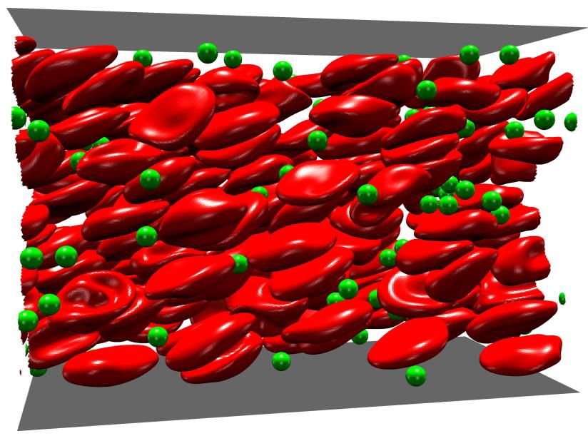
2                               H. Ye, Z. Shen and Y. Li

1. Introduction
   Margination, defined as migration of a particle in blood flow towards the periphery of
the blood vessel, allows the particle to come close to the endothelium, and then adhere to
the vessel wall (marquis Du Trochet 1824; Koumoutsakos et al. 2013). It is of significant
importance to understand such physiological processes for curing relevant diseases. For
example, in inflammation process, margination of leukocytes towards the vessel wall is
the precondition for organism to perform defense functions, such as adhering to vascular
endothelium and transmigrating into the tissues (Ley & Tedder 1995; Fedosov et al. 2012).
In atherosclerosis, the thrombosis, formed by the clot, is caused by the margination and
accumulation of numerous platelets responding quickly to events on the vessel wall (e.g.,
injury) (Wootton & Ku 1999; Fogelson & Neeves 2015). Additionally, margination has
extensive applications in microfluidic devices for the removal of pathogens and separation
of cells (Hou et al. 2010; Gossett et al. 2010; Bhagat et al. 2010).
   The root cause of margination has not been completely revealed so far. In the blood
flow, every component of blood such as plasma and red blood cells (RBCs) may contribute
to margination (Farutin & Misbah 2013). Generally speaking, three major factors:
hydrodynamic forces, wall effects and adhesive interactions between ligands and receptors
are considered to be responsible for the margination of micro-particles (MPs). Here,
another most important effect, Brownian interaction in nano-particles, can be ignored
due to the large size of MPs (Ramakrishnan et al. 2017). Hence, when placing the MP
in the blood flow through injection or other administration, the dynamics of MPs is
governed by the complex interplay among these three factors. The performance of the
MP will be affected by its physiological properties such as size, shape, stiffness and
surface functionality (also known as the ‘4S’ parameters) (Li et al. 2016; Ye et al.
2018c). These properties play different roles, depending on the specific physiological
conditions. For example, Decuzzi et al. (2010) found that in the in vivo experiment,
discoidal particles demonstrated strongest accumulation in most of the organs such as
spleen and kidney. While in the liver, cylindrical particles outperformed the other kinds
of particles. Therefore, investigations of the ‘4S’ parameters become crucial in the optimal
design of MPs acting as drug carriers in biomedical application.
   Among the ‘4S’ parameters, stiffness attracts relatively less attention compared to
other parameters. While it should play an important role in the margination process of
MPs. Due to the deformability, the symmetry of the Stokes flow is broken. According to
the mirror symmetry time reversal theorem proposed by Bretherton (1962), the elastic
MP will experience a lateral force in the near wall region. For example, usually the
leukocyte is assumed to marginate towards the vessel wall in blood flow (Fedosov et al.
2012; Freund 2007; Marth et al. 2016). Recently it has been discovered that the reversal
of margination (migration from the near wall region to center of vessel) happens, when
the stiffness is reduced by reorganization of cellular cortical actins (Fay et al. 2016).
   The dynamics of elastic particle is more complex than rigid one. The shape of elastic
MP is not given a priori and continuously deforms in flow. The evolution of shape is de-
termined by the dynamic balance between the interfacial force and fluid stress, depending
on the local flow environment. Additionally, a large number of RBCs occupies the blood
flow. Thus, the deformation and moving of RBCs influence the flow field around MPs.
Hydrodynamic interaction can also happen between RBCs and elastic MPs. Poiseuille
(1836) recognized that blood corpuscles in the capillaries tended to migrate away from the
Interplay of deformability and adhesion on localization of elastic micro-particles      3
wall due to deformation induced migration stemming from viscous effects. Nevertheless,
this stiffness dependent migration of particle attracts extensive attention very recently.
Owing to the similar behavior of RBCs under flow, a series of elastic particles, such
as capsules and vesicles, has been investigated in regards to their migration motion by
experimental (Abkarian et al. 2002; Coupier et al. 2008; Kantsler et al. 2008; Callens
et al. 2008), analytical (Olla 1997a,b; Qi & Shaqfeh 2017; Vlahovska & Gracia 2007;
Seifert 1999; Danker et al. 2009; Farutin & Misbah 2011, 2013), and numerical studies
(Cantat & Misbah 1999; Sukumaran & Seifert 2001; Secomb et al. 2007; Kaoui et al. 2008;
Doddi & Bagchi 2008; Nix et al. 2014; Zhao et al. 2011; Singh et al. 2014). Quantitative
determination of the deformation induced migration is instrumental to revealing the
underlying mechanism of the migration behaviors of erythrocytes and leukocytes in the
blood flow. Abkarian et al. (2002) used light microscopy to study the tank-treading
motion and deformation of vesicles in linear shear flow. Upon increasing the shear rate
of flow, the vesicle tilted with respect to the substrate, and further incrementation of
shear rate γ̇ made vesicle migrate away from substrate. These observations revealed
the existence of deformation induced migration. They found that the magnitude of the
deformation induced migration depended on the viscosity η of the fluid, the radius R
of the vesicle, the distance h from the substrate, and a monotonous decreasing function
 f (1 − v) of the reduced volume v. On the basis of these direct observations, Farutin &
Misbah (2013) derived the migration velocity of a vesicle near the wall. From the method
using stresslet of droplet in Couette device (Smart & Leighton Jr 1991), they employed
asymptotic method to derive the expression of migration velocity by determining stresslet
in a power series of shape parameter Γ of vesicles. Γ quantifies the deflation of vesicle
from sphere with the same volume. In the leading order of Γ , the migration velocity
∼ γ̇ R3 /h2 . While the theoretical analysis was implemented on the basis of assumption
that the deflation Γ is small. It means that if the shear modulus of the particles, such as
that of the capsule, is not high, the expression should not be valid. More recently, Singh
et al. (2014) corrected the analytical migration velocity by fitting the results obtained
from a series of numerical simulations for capsules with different elastic capillary numbers
Ca. They found that there existed a critical Cacr splitting the migration velocity into two
distinct regimes. When Ca < Cacr , migration velocity ∼ Ca and ∼ γ̇ R3 /h2 , which is similar
to the analytical relation for vesicles. While when Ca > Cacr , migration velocity ∼ Ca0.6
and ∼ γ̇ R2.35 /h1.35 . Hence, if the capsule is soft (large Ca), the analytic relation is not
valid for the capsule any more. Also, a detailed study for lift velocity of RBC through
simulations has been proposed by Qi & Shaqfeh (2017). Here, the elastic MPs pertain to
capsules, and will be discussed in detail later.
    According to Farutin & Misbah (2013), in addition to deformation induced migration,
hydrodynamic interaction is an additional governing mechanism of particle migration in
simple shear flow. Hydrodynamic interaction results in hydrodynamic diffusion, which
is induced by collisions between particles. Collision between two identical particles,
namely homogeneous collision such as capsules (Singh & Sarkar 2015) and vesicles
(Farutin & Misbah 2013) are investigated numerically and theoretically, respectively.
This homogeneous collision is not essential in particles migration and segregation, because
the migrations of two collision parts are the same. Kumar & Graham (2011, 2012b) and
Sinha & Graham (2016) extended this to heterogeneous collision between capsules with
the same volume, but different membrane rigidities and shapes, respectively. In the binary
suspension of soft and stiff capsules, the stiff particles were observed to accumulate in the
near wall region in the suspension of primarily soft particles. While soft particles were
found to concentrate on the centerline in the suspension of primarily stiff particles. This
segregation behavior was attributed to larger cross-stream displacement in heterogeneous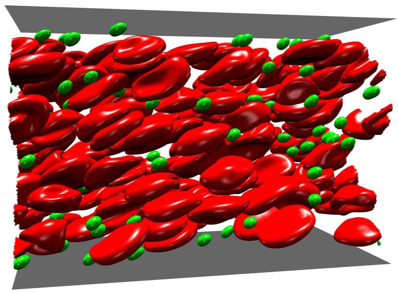
4                                H. Ye, Z. Shen and Y. Li
collisions of stiff particle than that of soft particles. Furthermore, Vahidkhah & Bagchi
(2015) proposed that binary collision between RBC and rigid MP should be one of the
reasons for the shape dependent margination behaviors of MPs. The result presented that
spherical and oblate MPs marginated more than prolate MPs after several collisions. In
terms of the elastic MPs, the collision between MPs and RBCs will be more complex,
and it should play an important role in margination behavior of elastic MPs. However,
it remains largely unexplored so far.
   After the particle marginates, it has a chance to interact with the vessel wall and adhere
to it, depending on the ligand-receptor binding properties. Adhesion behavior has been
extensively studied using the Bell model (Bell 1978), developed by adhesive dynamics
which was first employed to understand the dynamics of leukocyte adhesion under flow
(King & Hammer 2001; Hammer & Lauffenburger 1987; Hammer 2014). A number of
studies in drug delivery systems focus on the adhesion process (Charoenphol et al. 2010,
2012; Decuzzi & Ferrari 2006; Coclite et al. 2017; Fedosov 2010; Luo & Bai 2016). In
human blood, MPs with diameters of 3 µ m were found to be the ideal choice for spherical,
rigid particles to adhere to vessel walls rather than nano-particles (Charoenphol et al.
2010, 2012). In addition to spherical particles, Decuzzi & Ferrari (2006) investigated the
effects of particle size and shape on the adhesion behavior from the point of specific
adhesive interaction strength. They predicted that for a fixed shape (e.g., spherical
or ellipsoidal), there existed an optimal volume (size) making the adhesive strength
reach a maximum. Additionally, they found that non-spherical particles can carry a
larger amount of drugs than spherical particles with the same adhesive strength. More
recently, Coclite et al. (2017) constructed two-dimensional Lattice Boltzmann-immersed
boundary model to systematically predict the near-wall dynamics of circulating particles
with different shapes and adhesive strengths. As for adhesion behavior of deformable
particles, a variety of dynamic phenomena, including detachment, rolling, firm adhesion
and stop-and-go motion (Fedosov 2010; Luo & Bai 2016), were found. Luo & Bai (2016)
combined front-tracking-finite element method and adhesion kinetics model to investigate
capsule dynamics in flow and adhesive dynamics, respectively. It was found that, for the
particle with low Ca, deformation promoted the rolling-to-firm adhesion transition. While
the deformation would inhibit both rolling-to-firm adhesion and detachment-to-rolling
transition when the Ca of the particle was relatively high. Because the particle with high
Ca would collapse on the substrate, and in the middle of the particle, a ligand-receptor
free region formed. Further increment of Ca made the rolling motion vanish and the
particle shape largely deviate from spherical one.
   In general, margination is thought to be the necessary precondition for the adhesion
(Müller et al. 2016). Before particle can interact with vessel wall, it should marginate into
near wall region, e.g. cell-free layer (CFL) in the blood flow. The CFL is a thin layer near
vessel wall with no RBCs inside, which forms due to the deformability of RBCs. However,
adhesion can also, in turn, affect the margination process. In engineering applications,
micron-sized particles are often used as drug carriers due to their better performance over
nano-sized particles in the margination process (Tasciotti et al. 2008). The thickness of
the CFL is also measured in micron-size (about 1.5 ∼ 5.0 µ m) in human vasculature
(Fedosov et al. 2010b). Hence, when particle moves close to or enters the CFL, the
particle can interact with vessel wall through ligand-receptor binding. Additionally, in
terms of deformation of particle, the elastic MP may move away from wall to center
of blood flow due to deformation induced migration. But adhesion may play a role in
preventing it escaping from the CFL. Thus, the adhesion will affect the choice of elastic
MP located near the CFL: entering or departing from the CFL? Such phenomenon was
also reported in previous work (Müller et al. 2016), but without discussion. Researchers
Interplay of deformability and adhesion on localization of elastic micro-particles    5
pay more attentions to effects of particle ‘4S’ properties on either margination or adhesion
(Vahidkhah & Bagchi 2015; Decuzzi & Ferrari 2006; Müller et al. 2014).
   Considering above aspects, we focus on the performance of elastic MPs in the whole
process from margination to adhesion. We combine Lattice Boltzmann Method and
molecular dynamics to solve fluid dynamics and particles (RBCs and elastic MPs)
dynamics, respectively. These two parts are coupled by immersed boundary method.
In our simulation, the most expensive part is solving of fluid dynamics. The LBM
is adopted due to its high natural parallelism. In the past two decades, it has been
confirmed as an efficient and accurate numerical solver to handle fluid dynamics problems
(Higuera et al. 1989; Benzi et al. 1992; Chen & Doolen 1998). Its application in simulating
blood flow acquires significant progress (Aidun & Clausen 2010; Zhang et al. 2007, 2008;
Macmeccan et al. 2009; Clausen et al. 2010; Melchionna et al. 2010; Lorenz et al. 2009;
de Haan et al. 2018; Czaja et al. 2018). In the absence of large numbers of RBCs,
Melchionna et al. (2010) took a hydrokinetic approach (Bernaschi et al. 2009) to model
large scale cardiovascular blood flow to recognize the key relevance to the localization
and progression of major cardiovascular diseases, such as atherosclerosis. Borgdorff et al.
(2014) provided a multiscale coupling library and environment to make the simulation
of extra large scale vasculature network become doable. Furthermore, considering the
existence of RBCs, Zhang et al. (2008, 2007) conducted simulations from aggregation of
multiple RBCs to rheology of RBC suspension in two dimensional blood flow. Macmeccan
et al. (2009) and Clausen et al. (2010) extended it to three dimensional blood flow by
coupling LBM with finite element method. Additionally, adhesive dynamics of elastic
MPs to vessel wall is governed by the probabilistic model proposed by Hammer &
Lauffenburger (1987). The diameter of MPs are set as 2 µ m, and the hematocrit of
blood flow is 30%, in which the thickness of CFL is comparable to the particle size. To
clarify the influence of near wall adhesion on localization of MPs, the particle size and
blood flow conditions are fixed. The Ca is tuned by changing shear modulus of elastic
MPs, and we vary the adhesion strength to adjust the Ad. The interplay of adhesion
strength and particle deformability leads to two optimal margination regimes. One is
with moderate Ca and high Ad, and the other is with small Ca and moderate Ad. This
may shed light on the optimal design of MPs favoring high localization at wall in blood
flow.
   The paper is organized as follows. Section 2 describes the physical problem involving
elastic MPs transport in blood flow and numerical methods we employ to solve fluid
flow, particle dynamics and adhesive dynamics. We validate our computational method
in Section 3. Furthermore, Section 4 presents the margination and adhesion results. A
detailed discussion of underlying physical mechanisms is also provided. In section 5,
conclusions are given.

2. Physical Problem and Computational Method
                                  2.1. Physical problem
  In the blood flow, most parts of the vessel are occupied by a large number of RBCs. In
the normal human blood vessel, the volume fraction (hematocrit Ht) is about 20 ∼ 45%.
Under the interplay effect of the flow and vessel wall, RBCs move from the near wall
region to the center of vessel due to deformation induced migration. It results in the
formation of a cell-free layer (CFL). The CFL plays a role as a lubricant layer and
reduces the blood flow resistance, which is also called Fahraeus-Lindqvist effect (Fåhræus
& Lindqvist 1931). When the elastic MPs, acting as drug carriers, are injected into a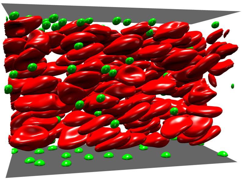
6                                       H. Ye, Z. Shen and Y. Li
    (a)
                                                                                               Ligands

                                                               Biological bond                 Receptors

        z

            y
    x

    (b)              Cell layer ( C )

                      Cell-free layer ( F )
                      ( ~2.8 "m )
                                                                          ! Adhesion layer
                                                                                 ( ~1.0 "m )

Figure 1. Transport of elastic MPs in blood flow. (a) Computational model of margination and
adhesion of elastic MPs in blood flow. Zoom-in figures give the detailed adhesion behavior of
elastic MP under stochastic ligand-receptor binding effect. (b) Schematic of transport process of
elastic MP from center of blood stream (denoted as C) to cell-free layer (F), and then reaching
adhesion layer.

vein, they move with bulk flow as shown in figure 1a. The elastic MPs deform under
the shear stress and collide with RBCs. And the deformation depends on the local flow
environment. Additionally, the MPs may move in the cross-stream direction, migrating
either towards the wall or to the center of the channel. Once MPs migrate to the near wall
region, i.e., CFL, the ligands decorated on their surfaces have the chance to interact with
the receptors on the endothelial cell distributed on the vessel wall (figure 1a). And this
ligand-receptor binding is required for the further release of drug molecules into tumor
sites through vascular targeting strategy (Schnitzer 1998; Neri & Bicknell 2005). However,
reaching the CFL cannot guarantee that such interactions will occur. Only when the MP
reaches a closer distance to the vessel wall, in which ligands can interact with receptors,
the interaction occurs. This distance is determined by the reaction distance between
ligands and receptors. We name the layer within this distance as adhesion layer (χ ).
Usually the thickness of the adhesion layer is in the range of tens to hundreds nanometers
(Decuzzi & Ferrari 2006; Müller et al. 2014, 2016). Here, it is set as 1.0 µ m according to
the reaction distance we used in the computational model. And it is reasonable compared
to that in previous work of Müller et al. (2014).
   The numerical study is employed to study the transport of elastic MPs due to its
flexibility in tuning the properties of MPs and adhesive interactions. The blood flow is
considered a suspension of RBCs. Limited to computation resource, a small part of the
vessel is taken into account and modeled as a rectangular channel. The size of the channel
is of height 36 µ m, width 27 µ m and length 54 µ m. Periodical boundary conditions are
applied in width (x) and length (y) directions. Height (z) direction is bounded by two
flat plates. The bottom plate (vessel wall, also namely substrate) is fixed and the flow is
driven by the moving of upper one with a constant velocity U. In all of the simulations,
shear rates stay at 200 s−1 . 162 RBCs and 80 identical elastic MPs are placed inside the
channel. The hematocrit (volume fraction of RBCs) is about 30%. MPs are initially set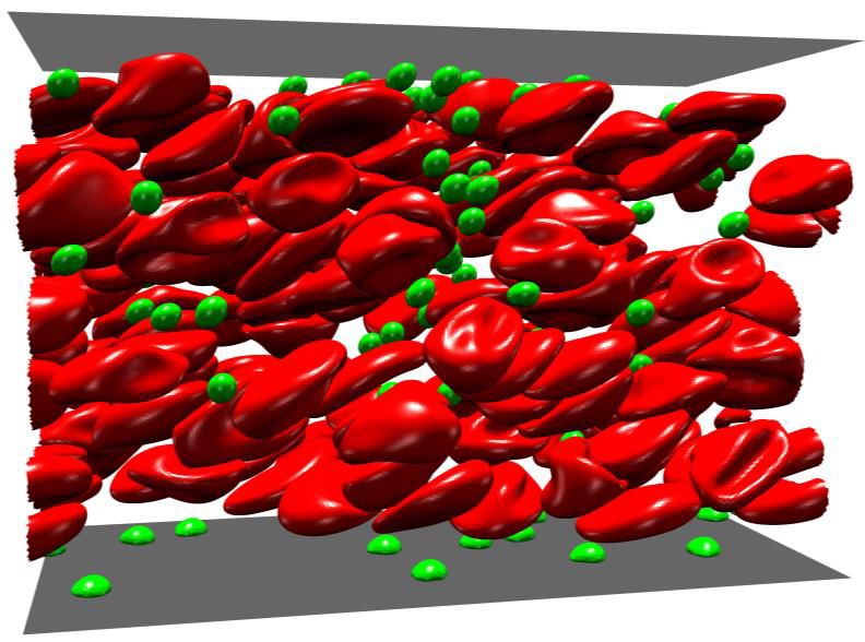
Interplay of deformability and adhesion on localization of elastic micro-particles        7

Parameters                                            Simulation                Physical Value
Equilibrium length of bond (l0 )                           1                        250 nm
Bond strength (ks )                             2.6 × 10⁻⁵ ∼ 1.2 × 10⁻² 1.64 × 10⁻⁹ ∼ 7.56 × 10⁻⁶ N/m
Reactive and rupture distance (don and do f f )            4                          1µ m
On strength (σon )                                      0.7305                  1.9 × 10⁻⁷ N/m
Off strength (σo f f )                                  0.7305                  1.9 × 10⁻⁷ N/m
Unstressed on rate (kon0 )                               3.75                    1.3 × 10⁶ s−1
Unstressed off rate (ko0 f f )                           0.05                    1.8 × 10⁴ s−1
Ligand density (nl )                                     4.11                     66 mol/µ m2
Receptor density (nr )                                    1.0                     16 mol/µ m2
           Table 1. Parameters used in adhesive model for ligand-receptor binding.

to spherical shape with radius 1 µ m, and their total volume fraction is about 0.64% in the
channel. Additionally, on the surfaces of MPs and substrate, the ligands and receptors
are uniformly distributed, respectively. The densities of ligands and receptors are listed
in Table 1.

                                2.2. Computational method
2.2.1. Lattice Boltzmann method for fluid flow
   The RBCs are immersed within blood plasma in the blood flow. The other components,
such as the white blood cells and platelets are negligible due to their low volume fractions
compared to that of RBCs. The plasma is usually considered as a Newtonian fluid. And
its dynamics is described by the continuity equation and incompressible Navier-Stokes
(NS) equation:
                                          ∇ · u = 0,                               (2.1)
                                ∂u
                             ρ       + ρ u · ∇u = −∇p + µ ∇2 u + F,                (2.2)
                                 ∂t
where ρ is the plasma density, u and p represent the velocity and pressure of the flow,
respectively. The term F on the right-hand side of Eq. (2.2) is the external force. µ is
the dynamic viscosity of the plasma and it is set as 1.2 cP. The Lattice Boltzmann (LB)
method is employed to solve the NS equation due to its high efficiency and accuracy
to handle incompressible Newtonian flow (Higuera et al. 1989; Benzi et al. 1992; Chen
& Doolen 1998). By discretizing velocity of the linearized Boltzmann equation, a finite
difference scheme is obtained:
                                                          ∆t
                      fi (x + ei ∆ t,t + ∆ t) = fi (x,t) − ( fi − fieq ) + Fi ,    (2.3)
                                                          τ
where fi (x,t) is distribution function and ei is the discretized velocity. In the current
simulation, the D3Q19 velocity model is used (Mackay et al. 2013), and the fluid particles
have possible discrete velocities stated in Mackay et al. (2013). τ denotes the non-
dimensional relaxation time, which is related to the dynamic viscosity in NS equation as
the form:
                                                   1
                                     µ = ρ c2s (τ − )∆ t.                            (2.4)
                                                   2
  eq
fi (x,t) is the equilibrium distribution function and Fi is the discretized scheme of
external force. In current simulation, the equilibrium distribution function adopts the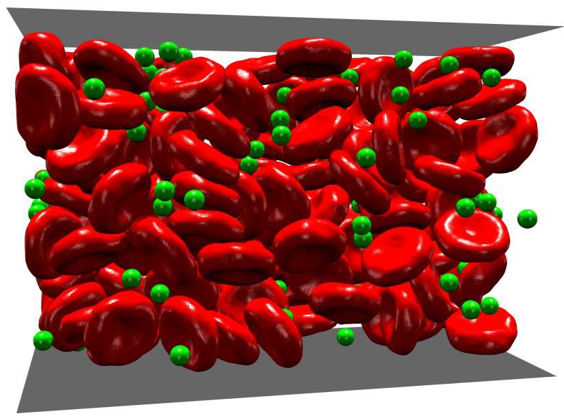
8                                 H. Ye, Z. Shen and Y. Li
form:
                                         [                          ]
                                             ei · u (ei · u)2 (u)2
                        fieq (x,t) = ωi ρ 1 + 2 +            −        ,                 (2.5)
                                              cs      2c4s     2c2s
where the weighting coefficients ωi = 1/3 (i = 0), ωi = 1/18 (i = 1√
                                                                   − 6), ωi = 1/36 (i =
7 − 18). The term cs represents the sound speed which equals ∆ x/( 3∆ t). The external
forcing term can be discretized by the form (Guo et al. 2002):
                                         [                   ]
                                    1      ei − u (ei · u)
                         Fi = (1 − )ωi           +         ei · F.                (2.6)
                                   2τ        c2s    c4s

  Eq. (2.3) is advanced through the algorithm proposed by Ollila et al. (2011). Here, the
solver of LB is embedded in Large-scale Atomic/Molecular Massively Parallel Simulator
(LAMMPS) (Plimpton 1995), which is implemented by Mackay et al. (2013). After the
particle density distributions are known in the whole fluid domain, the properties of fluid,
such as fluid density and velocity can be calculated as:
                                                       1            1
                             ρ = ∑ fi , u =
                                                       ρ∑
                                                           fi ei +    F∆ t.             (2.7)
                                    i                    i         2ρ

2.2.2. Coarse-grained models for RBC and MP
   To capture the dynamics and deformation of RBCs and elastic MPs, we develop a
coarse-grained model and implement it into LAMMPS (Ye et al. 2018b). The RBC is
modeled as liquid-filled coarse-grained membrane, and its equilibrium shape is biconcave.
The diameter of a RBC is 7.8 µ m, and the thickness is about 2.1 µ m. The surface area
and volume of RBC are 134.1 µ m2 and 94.1 µ m3 , respectively (Evans & Skalak 1980).
In the simulation, the membrane is discretized into 3286 vertices and 6568 triangular
elements.
   To capture the in-plane shear property of RBC, a stretching potential Ustretching is used.
It includes two parts: attractive nonlinear spring potential - wormlike chain model (WLC)
and repulsive power potential - power function (POW) (Fedosov et al. 2010a, 2011b).
They can be expressed as:

                                        kB T lm 3x2 − 2x3         kp
                           UW LC =                        , UPOW = ,                    (2.8)
                                          4p      1−x              l
where kB T is the basic energy unit. x = l/lm ∈ (0, 1), l is the length of the spring and lm
is the maximum spring extension. p is the persistent length, and k p is the POW force
coefficient. Applying bending potential

                           Ubending =         ∑        kb [1 − cos(θk − θ0 )],          (2.9)
                                            k∈1...Ns

the out-of-plane bending property of RBC is reflected. kb is the bending stiffness. θk is
dihedral angle between two adjacent triangular elements, and θ0 is the initial value of
dihedral angle. In the following, subscript 0 represents the corresponding initial value.
Ns denotes the total number of dihedral angles.
  Besides, the bulk properties, such as surface area and volume conservation are ensured
by introducing the penalty forms:

                                            kd (Ak − Ak0 )2 ka (At − At0 )2
                       Uarea =     ∑             2Ak0
                                                           +
                                                                 2At
                                                                            ,         (2.10)
                                 k=1...Nt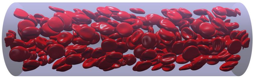
Interplay of deformability and adhesion on localization of elastic micro-particles   9
and
                                                   kv (V −V0 )
                                      Uvolume =                ,                      (2.11)
                                                       2V0
where the first term in Eq. (2.10) represents the local area constraint, Ak and Ak0 denote
the area of k-th element and its initial area, respectively, and kd is the corresponding
spring constant. The second term in Eq. (2.10) is the global area constraint. At is the
total area, and ka is the spring constant. In Eq. (2.11), kv is the spring constant and V is
total volume.
  Then the total energy U is:

                        U = UW LC +UPOW +Ubending +Uarea +Uvolume .                   (2.12)

The nodal forces exerted on each vertexes of the RBC membrane are derived by:

                                        fi = −∂ U(Xi )/∂ Xi ,                         (2.13)

where Xi denotes the vertex of RBC membrane. Thus, if we know the position of
membrane vertexes, we can calculate the nodal force according to Eq. (2.13). The detailed
derivation of the force formulae such as two-point stretching force and three-point bending
force are presented in Ye et al. (2018b).
  The elastic MPs adopt the same model as RBCs, but with 828 vertices and changeable
in-plane shear strength. Before we choose the parameters for the coarse-grained model
of RBCs and elastic MPs, we should know the corresponding macroscopic properties
through experiments as a priori. According to the relationship between coarse-grained
model parameters and macroscopic properties (Allen & Tildesley 1989; Dao et al. 2006;
Fedosov et al. 2010a)
                          √                                       √
                            3kB T     x0           1        1    3 3k p
                    µ0 =           (         −           + )+           ,
                          4plm x0 2(1 − x0 )3 4(1 − x0 )2 4        4l03
                     K = 2µ0 + ka + kd ,
                           4K µ0
                     Y=           ,                                                   (2.14)
                          K + µ0
where µ0 is the shear modulus, K represents the area compression modulus and Y denotes
the Young’s modulus. Therefore, the potential parameters can be chosen on the basis of
the physical quantities. The parameters used in the simulation are listed in Table. 2.
   The accuracy of this model for RBC and elastic MP has been validated in our previous
works (Ye et al. 2018a,b, 2017a). In Section 3, we will show two more validations to
confirm the convergence of both fluid and membrane meshes and modeling of rheology
of blood flow. The details about the computational efficiency and cost are discussed
in Section 5 and Ye et al. (2018b). In addition to the above potentials, it is necessary
to employ inter-molecular interactions between RBCs to characterize their interactions.
Here we use the Morse potential as inter-molecular interactions (Liu & Liu 2006; Fedosov
et al. 2011b; Tan et al. 2012), with the form

                          Umorse = D0 [e−2β (r−r0 ) − 2e−β (r−r0 ) ], r < rc ,        (2.15)

where D0 represents the energy well depth and β controls the width of potential well,
r is the distance between two particles and r0 is the equilibrium distance, rc is the
cutoff distance. Additionally, a short range and pure repulsive Lennard-Jones potential
is applied to prevent the overlap between RBCs and MPs (Ye et al. 2018b).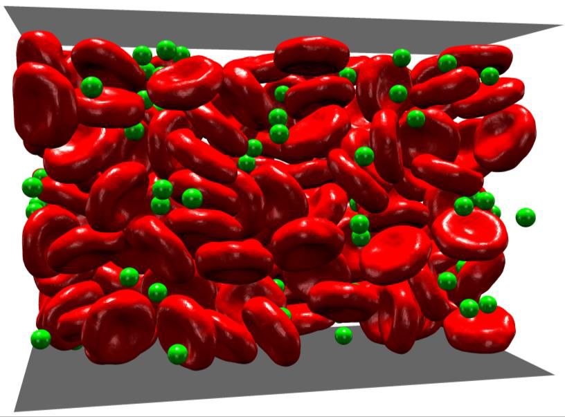
10                                 H. Ye, Z. Shen and Y. Li

            Parameters                 Simulation        Physical Value
            RBC diameter (Dr )             32               8 × 10⁻⁶ m
            MP diameter (2R)                8               2 × 10⁻⁶ m
            RBC shear modulus (µr )       0.01           6.3 × 10⁻⁶ N/m
            MP shear modulus (µ0 )     10−4 ∼ 1.0 6.3 × 10⁻⁸ ∼ 6.3 × 10⁻⁴ N/m
            Energy scale (kB T )       1.1 × 10⁻⁴       4.14 × 10⁻²¹ N · m
            Viscosity of fluid (η )      0.167              0.0012 Pa · s
            Area constant (ka )          0.0075         4.72 × 10⁻⁶ N/m
            Local area constant (kd )    0.367          2.31 × 10⁻⁴ N/m
            Volume constant (kv )        0.096               249 N/m2
            RBC bending constant (kb )   0.013            5 × 10⁻¹⁹ N · m
 Table 2. Coarse-grained potential parameters for red blood cells and elastic MPs, and their
                               corresponding physical values.

2.2.3. Immersed boundary method for fluid-structure interaction
   The immersed boundary (IB) method is used to couple LBM with LAMMPS to account
for fluid-structure interaction (Peskin 2002; Krüger et al. 2011, 2014; Ye et al. 2017b).
We use the Lagrangian (X) and Eulerian (x) mesh points in the computational domain
to represent RBC (or MP) and fluid particles, respectively. The Eulerian fluid mesh is
uniform and the resolution is ∆ x = 250 nm in all directions. The Lagrangian mesh for RBC
or MP is generated by MATLAB code (Persson & Strang 2004; Persson 2005). The mesh
is approximately uniform and the mesh size is set about ∆ X = 0.6 ∼ 0.8∆ x. Then there are
about 32 Eulerian points across one RBC in diametral direction. It is sufficient to resolute
the deformation and motion of RBC (Macmeccan et al. 2009; Vahidkhah & Bagchi 2015).
The coupling is fulfilled by the interpolation of velocity and force distribution between
Lagrangian and Eulerian mesh points (Mittal & Iaccarino 2005).
   To ensure no-slip boundary condition, the membrane vertices X with Lagrangian
coordinate s should move at the same velocity as the fluid around it. That is
                                      ∂ X(s,t)
                                               = u(X(s,t)).                            (2.16)
                                         ∂t
The velocity can be interpolated by the fluid velocity through a smoothed Dirac-Delta
function δ :
                                          ∫
                           u(X,t) =               u(x,t)δ (x − x(X,t))d Ω .            (2.17)
                                              Ω
This condition will cause the membrane to move and deform. The membrane force density
F(s,t) is obtained by derivation of potential functions as Eq. (2.13), and is distributed to
the surrounding fluid mesh points by
                                          ∫
                         f f si (x,t) =       F f si (X,t)δ (x − x(X,t))d Ω .          (2.18)
                                          Ω

2.2.4. Adhesive model for ligand-receptor binding
   The ligand-receptor binding is described by the association and dissociation of bi-
ological bonds. And it is governed by the probabilistic adhesion model (Hammer &
Lauffenburger 1987). Figure 1(a) gives the schematic of the adhesive model. When the
ligands on the MP approach the receptors on the vessel wall, they have the chance to
bind together. And it is determined by the probability Pon . Reversely, the existing bond
Interplay of deformability and adhesion on localization of elastic micro-particles 11
has a probability Po f f to break. They can be expressed as:
{ {
1 − e−kon ∆ t , l < don 1 − e−ko f f ∆ t , l < do f f
Pon = , Po f f = , (2.19)
0, l > don 0, l > do f f
where ∆ t is the time step in simulation, don and do f f are the cutoffs for bond creation
and breakup, respectively. kon and ko f f are the association and dissociation rates with
the forms:
0 σon (l − l0 )2 σo f f (l − l0 )2
kon = kon exp(− ), ko f f = ko0 f f exp( ), (2.20)
2kB T 2kB T
where σon and σo f f are the effective on and off strengths, representing a decrease and
increase of the corresponding rates within don and do f f , respectively. kon 0 and k0
o f f are
the reaction rates at the equilibrium length l = l0 between ligand and receptor. The
mechanical property of biological bond is described by a harmonic spring. l0 is the
equilibrium length, and the force exerted on the receptor and ligand is: Fb = ks (l − l0 ).
Here, ks represents the adhesive strength. This model and the relevant parameters (c.f.
Table. 1) are chosen according to previous works of Fedosov (2010) and Fedosov et al.
(2011a).
There are three dimensionless parameters, including
Reynolds number : Re = ρ γ̇ R2 /µ , (2.21)
Capillary number : Ca = µ γ̇ R/µ0 , (2.22)
Adhesion number : Ad = ks /µ γ̇ R. (2.23)
Considering the physiological environment surrounding the cell, the fluid flow is
considered as a Stokes flow. Thus, Re is very small, and we fix its value Re = 0.0134
to approximately represent the Stokes regime. The capillary number represents the ratio
of shear stress exerted on the surface of elastic MP to elastic force induced by deformation
of elastic MP. µ0 is the shear modulus of the MP. The higher the Ca, the softer of the
particle. The adhesion number denotes the ratio of adhesive strength to shear stress of
flow. Thus, the higher the Ad, the stronger the adhesion strength. In our simulations, Ca
is tuned by varying shear modulus µ0 , and Ad is varied by changing adhesive strength
ks .
3. Validation of Numerical Method
The grid independence studies of fluid and RBC membrane are conducted. We perform
a case study that a single RBC with diameter (Dr ) moves in simple shear flow (v(z) = γ̇ z)
shown in figure 2(a). Here the RBC is discretized with different vertexes presented in
figure 2(b). To exclude the size effect of the channel, we adopt the same channel and
same shear rate as the margination studies of MPs. First, we vary the mesh size ∆ x of
the fluid, and track the trajectories of the center of RBC in height direction (z-direction).
Figure 2(c) shows that when the mesh is coarse (∆ x = 1/8Dr ), the trajectory is obviously
different from those with fine meshes, and it is not smooth compared to those with fine
meshes. Further increase of mesh resolution (∆ x = 1/16Dr ) leads to a more consistent
trajectory, and only small difference of trajectory exists between it and finer mesh. When
the mesh resolution increases to ∆ x = 1/32Dr , the difference between it with the finer mesh
can be negligible. Thus, current study adopts the mesh size ∆ x = 1/32Dr . Furthermore,
we change the discretized vertexes of the RBC membrane. Four cases V = 766, 1418, 3286
and 9864 are investigated here. V and T represent the numbers of vertex and triangular12 H. Ye, Z. Shen and Y. Li
(a) (b)
V = 766 V = 1418
z
x y
V = 3286 V = 9864
(c) (d)
Figure 2. Grid independence studies. (a) Model of motion of single RBC in simple shear flow.
(B) Discretization of RBC membrane with different vertexes. (c) Grid independence of fluid
mesh. (d) Grid independence of RBC discretization.
element of RBC membrane, respectively. Again, we track the trajectories of the center
of RBC in the height direction. We find that the discretization of the membrane has
weak influence on the motion of RBC under current scheme (766 < V < 9864). There
is only a small difference for the case of V = 766, comparing to other cases. To ensure
enough convergence of membrane mesh, we adopt a relatively fine mesh V = 3286. In the
following simulations, the fluid mesh size is ∆ x = 1/32Dr and the discretization of RBC
membrane is V = 3286.
Here, we conduct the Fahraeus effect and Fahraeus-Lindqvist effect of blood flow with
different hematocrits (15% and 30%) in the tube with different diameters (10 µ m, 20 µ m
and 40 µ m) to validate our numerical method in terms of rheology of blood flow. The
length of the tube is fixed as three times of the diameter.
The Fahraeus effect presented an increased value of discharge hematocrit (Hd ) mea-
sured at the tube exit in comparison with that before the tube entrance. It was first
discovered in in vitro experiments of blood flow in tube (Fåhraeus 1929). In our sim-
ulation, we take the same definition as that in Fedosov et al. (2010b) to calculate the
discharge hematocrit.
v̄c
Hd = Ht , (3.1)
v̄
where v̄ = Q/A is the mean velocity of the blood flow, and v̄c is the average cell velocity
averaged in time in the steady-state regime.
The Fahraeus-Lindqvist effect stated that apparent blood viscosity decreased withInterplay of deformability and adhesion on localization of elastic micro-particles 13
(a)
D !"# = 10 $% D !"# = 40 $%
D !"# = 20 $%
(b) (c)
Relative apparent Viscosity hrel
0.6 3.0
Fedosov et al. (2010), Ht = 15%
Fedosov et al. (2010), Ht = 15%
Discharge hematocrit Hd
Ht = 30%
Ht = 30%
Pries et al. (1992), Ht = 15%
Pries et al. (1992), Ht = 15%
Ht = 30%
0.5 Ht = 30%
2.5 Present simulation, Ht = 15%
Present simulation, Ht = 15%
Ht = 30%
Ht = 30%
Empirical viscosity, Ht = 15%
Ht = 30%
0.4 Czaja et al.(2018), Ht = 30%
2.0
0.3
1.5
0.2
1.0
0 10 20 30 40 50 0 10 20 30 40 50
Tube diameter (mm) Tube diameter (mm)
Figure 3. Fahraeus and Fahraeus-Lindqvist effects. (a) Snapshots to show the tube flow with
different diameters under hematocrit 15%. (b) Fahraeus effect: discharge hematocrit comparison.
(c) Fahraeus-Lindqvist effect: relative viscosity validation.
decrease of tube diameter found in experiments (Fåhræus & Lindqvist 1931; Pries et al.
1992, 1994). And it is usually convenient to calculate the relative apparent viscosity to
investigate this effect, which is defined as:
ηapparent
ηrel = , (3.2)
η plasma
where the apparent viscosity ηapparent = ∆ PDtube
2 /32v̄L. ∆ P and L are pressure difference
between inlet and outlet of the tube and length of the tube, respectively.
In figure 3(a), we show the snapshots of blood flow in tube with different diameters
under hematocrit 15%. We calculate the discharge hematocrit and relative viscosity of
the blood flow, and compare our results with those in experiment (Pries et al. 1992)
and numerical (Fedosov et al. 2010b; Czaja et al. 2018) studies in figure 3(b) and (c).
As for the relative viscosity of the blood flow, we also provide the empirical viscosity
from experiment (Pries et al. 1994). We find that our results are more consistent with
empirical value under low hematocrit 15% compared with that under hematocrit 30%.
What’s more, the results have a more consistence with the numerical results than
that with empirical results. The discrepancies existed between numerical simulations
and experiments may be induced by the interaction between RBC and tube wall, and
estimation method in experiments (Fedosov et al. 2010b). However, current study has
adequate accuracy to model the blood flow from above comparison.
4. Results and Discussion
We study the margination behaviors of elastic MPs (i) without (Ad = 0) and (ii) with
(Ad = 0.07 ∼ 32.8) adhesion. The stiffness of the elastic MPs is varied by changing the14 H. Ye, Z. Shen and Y. Li
z
y
x t = 1.0 s t = 2.0 s
t=0s
Figure 4. Snapshots to show the margination behavior of elastic MP (Ca = 0.0037) without
effect of adhesion.
shear modulus µ0 , which makes Ca range from 0.00037 to 3.7. It corresponds to the shear
modulus of MP from 6.3 × 10⁻⁴ to 6.3 × 10⁻⁸ N/m (note that shear modulus of RBC
is 6.3 × 10⁻⁶ N/m). The elastic MPs are randomly placed among RBCs in the whole
channel at the beginning of all simulations. For MPs with different shear moduli, they
have the same initial configurations. It can eliminate the influence of initial condition on
the margination results.
4.1. Margination of elastic MPs without adhesion
The margination of MPs without adhesion is first investigated. The margination
process of a typical case of MPs with Ca = 0.0037 is shown in figure 4. In these snapshots,
at t = 0 s, we can see that MPs are randomly distributed as well as RBCs. The RBCs
and MPs are considered at their equilibrium states. The shapes of RBCs and MPs are
biconcave and spherical, respectively. At time t = 1.0 s, the fluid flow is developed. A large
deformation has been observed for RBCs. Under the shear flow, we find that RBCs align
their major axes along the flow direction. Though the deformation of MPs is small due
to their high stiffness (small Ca = 0.0037), it should deform under the shear stress. And
the deformation will be significant for case with high Ca. In addition to the deformation,
RBCs and MPs both demonstrate cross-stream migration, but towards the opposite
directions. RBCs migrate from near wall region to the center of channel, while MPs
move towards the wall. We also find that the CFL becomes clear and some MPs have
reached the CFL quickly. As simulation time further advances, at t = 2.0 s, the CFL is
fully developed and MPs start to accumulate at the CFL.
Localization of MPs at wall is characterized by margination probability Φ (t), which is
defined as:
n f (t)
Φ (t) = , (4.1)
N
where n f (t) represents the number of MPs with centers locating in CFL at time t, and
N denotes the total number of MPs in the channel. Before quantifying the margination
probability, the thickness of CFL is estimated in the absence of MPs. We use the same
method proposed by Fedosov et al. (2010b), the thickness of CFL is about 2.8 µ m for
current blood flow with Ht = 30%. This is consistent with previous numerical studies
(Lee et al. 2013; Müller et al. 2014). Figure 5(a) gives the evolution of margination
probabilities Φ for three different stiffnesses (Ca = 0.00037, 0.037 and 3.7). We find that
the margination process can be split into two stages. In the first stage, the margination
probability increases very fast, which signifies that there are more and more particles
moving from the center to CFL. We note that, in this stage, the margination probabilities
of softer particles increase faster (Ca = 0.037 and 3.7) than that of stiff particles (Ca =
0.00037). However, the duration of this stage for stiff particles is longer than those of
soft particles. Therefore, when the first stage ends, the margination probability of stiffInterplay of deformability and adhesion on localization of elastic micro-particles 15
´10-6
(a) 0.7
Ca = 0.00037
(b) 1.0
Ca = 0.00037
0.6 = 0.037 = 0.0037
= 3.7 0.8 = 0.037
0.5 = 0.37
áD Z ñ (cm )
2
= 3.7
0.4 0.6
F
2
0.3 0.4
0.2
0.2
0.1
0.0 0.0
0 1 2 3 4 5 6 0.0 0.5 1.0 1.5 2.0 2.5 3.0 3.5
t (s) t (s)
(c) 0.7 (d) 0.65
Ca = 0.00037
0.6 = 0.037
= 3.7 0.60
0.5
0.55
Probability
C-F
0.4
áFñ
0.50
0.3
0.45
0.2
F-C
0.1 0.40
0.0 0.35 -4
0 1 2 3 4 5 6 10 10-3 10-2 10-1 100
t (s) Ca
Figure 5. Margination behavior of elastic MPs with different stiffnesses. (a) Evolution of
margination probabilities for elastic MPs. (b) Mean square displacement of elastic MPs during
margination. (c) Probabilities of two types of motion: center to cell-free layer (C-F) and cell-free
layer to center (F-C). (d) Time-averaged margination probability at steady-state regime.
particles is higher than those of soft ones. In the second stage, margination probabilities
of both stiff and soft particles increase slower than those in the first stage. And the
growth rates for these particles are almost the same.
To investigate this stiffness-dependency of margination behavior, the mean square
displacements (MSDs) for MPs with different stiffnesses are calculated. The deformation
of RBCs in the blood flow induces the fluctuation of flow around them. It is considered
as the root cause of migration of rigid particles such as platelets in blood flow (Zhao
et al. 2012). From figure 5(b), we find that there are no obvious difference among MSDs
for all of the MPs. At the initial stage (t < 1.0 s), the MSDs are almost the same.
After that, the MSDs for MPs become different, but with only small variations. We
calculate the diffusivities, defined as D =< ∆ z2 > /2t, and they range from about 0.9
to 1.2 × 10⁻⁷ cm−2 s−1 for these MPs. This is in good agreement with previous studies
(Vahidkhah & Bagchi 2015; Zhao & Shaqfeh 2011). The diffusivity is about 2 orders
of magnitude higher than the Brownian diffusivity, which means the existence of RBCs
augments the diffusion of MPs. However, from these results, RBCs augmentation of
diffusion is stiffness independent. Thus, the diffusion can not solely explain the observed
stiffness-dependency of margination behavior.
To gain a better insight into the margination behavior, the motion types of MPs
in blood flow are studied. Compared to rigid particles in blood flow, elastic MPs may16 H. Ye, Z. Shen and Y. Li experience deformation induced migration, which can drive them to move away from the vessel wall (Kumar & Graham 2012b; Coupier et al. 2008). And this is the essential mechanism for CFL formation in blood vessel. Here the motion of elastic MPs can be classified into four types: (i) staying in the center; (ii) staying in the CFL; (iii) moving from center to CFL (C-F); and (iv) moving from CFL to the center (F-C). Obviously, the first two types cannot contribute to the localization of MPs at wall. The margination probability is attributed to the difference between the last two types as shown in figure 5(c). We find that the probabilities of F-C motion for all of the elastic MPs are the same and the values are almost 0. It indicates that there are only few particles migrating from CFL to the center region. We also observe that the C-F motion has the same tendency as the margination probability Φ . All these results lead to the conclusion that localization of MPs at wall in current study is determined by the C-F motion. This is different from our previous study in Ye et al. (2017a), in which F-C motion at some time can dominate the margination behavior of particles. The reason causing this difference mainly lies on the size of the particle and hematocrit of blood flow. If the size of the particle is large (2 µ m in diameter), and the hematocrit is high (30%), there is no available space for the particle to stay in the center of the channel. Because, under shear flow, the most parts of center region are occupied by RBCs. Hence, F-C motion is not significant in present study. To quantify the stiffness effect on margination probability, the mean margination probabilities < Φ > are calculated and given in figure 5(d). The mean value takes the time-averaged value of margination probability, which is estimated in a time interval within the steady-state regime. We can see that the margination process of MPs reaches steady state after about t = 2.5 s. The localization of MPs at wall decreases dramatically when the particles are very stiff (small Ca). While with further decrease of stiffness (increase of Ca), there is no obvious change of the margination probability. The underlying mechanism of this stiffness-dependency of margination behavior relies on the interplay of collision with RBCs and deformation induced lateral migration of elastic MPs (Qi & Shaqfeh 2017). At the beginning of the simulation, the RBCs near the wall of channel sense the shear flow, and then deform under the shear stress. The existence of wall makes RBCs move away from wall, and then the CFL forms. According to previous study in Katanov et al. (2015), the time needed to fully form CFL is about 0.8 s under the conditions (channel size and hematocrit) in current study (Ye et al. 2017a). It signals that the first stage of margination probability corresponds to the development of CFL (c.f., figure 5(a)). In this stage, a large number of RBCs move from near wall region to center of channel. The migration of RBCs should induce reverse flow moving from center to CFL in the regions around RBCs, due to the mass conservation of the fluid. Hence, if the MPs locate in these reverse flow regions, they will move along with the flow from center to CFL. This phenomenon looks like the exclusion effect that particles are excluded by RBCs from near wall region to center of the channel (Crowl & Fogelson 2011). Specifically, the exclusion effect appears more significant for soft particles than stiff particles. Here soft MPs have stronger alignment to flow due to deformation. This is the reason why, in the first stage, the soft MPs marginate faster than stiff ones. In the second stage, the CFL is fully formed and the flow is fully developed. The soft MPs in the near wall region may experience the deformation induced migration due to the existence of the wall. This results in the low accumulation of soft MPs in the CFL. However, when the stiffness of MPs decreases to a critical value (about Ca = 0.037), the deformation induced migration dominates the motion of MPs. Therefore, under this circumstance, changing stiffness of MPs will not result in an obvious difference of the margination probability.
Interplay of deformability and adhesion on localization of elastic micro-particles 17
(a)
z
y
x
(b)
t=0s t = 1.0 s t = 2.0 s
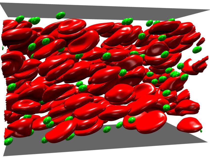
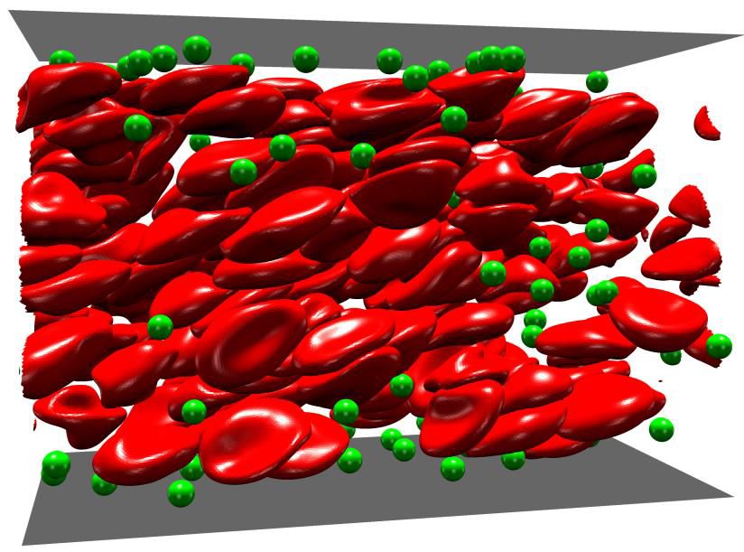
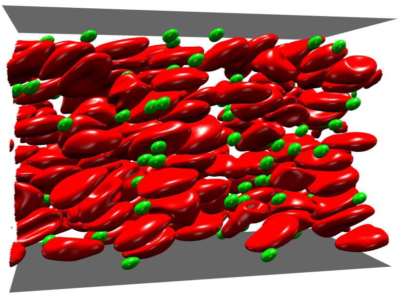
Figure 6. Snapshots for the margination behavior of elastic MPs (Ca = 0.37) under influence of
adhesion (a) Ad = 0.07 and (b) Ad = 32.8.
4.2. Adhesion effect on localization of elastic MPs at wall
In the figure 5(a), it is obvious that the evolution of margination probability oscillates.
In some time intervals, the oscillation amplitude can reach about 20% of the margination
probability. It indicates that many MPs are traveling between the center of the channel
and CFL. Under this circumstance, MPs near the CFL have chance to interact with the
vessel wall through ligand-receptor binding. Since the diameter of MP is 2.0 µ m, when it
moves near the CFL, a part of its surface will locate inside the adhesion layer according
to the thicknesses of CFL (2.8 µ m) and adhesion layer (1.0 µ m).
To have a direct comparison, figure 6 presents adhesion effect on the localization of
elastic MPs. In figure 6(a), and figure 6(b), the stiffnesses of MPs are the same Ca = 0.37,
while the adhesion strengths are different: (a) Ad = 0.07, and (b) Ad = 32.8. We find that
there are more MPs entering and staying inside the CFL when increasing the adhesion
strength Ad. With small Ad = 0.07, when MPs move into CFL, only a small contact area
forms between MP and substrate. The ligand-receptor binding is not strong, and these
MPs move freely near the substrate. However, with strong adhesion Ad = 32.8, the MPs
collapse on the substrate like a droplet on the ground. It should be emphasized that this
collapse phenomenon only happens for soft MPs. If the MP is stiff or rigid, it can not
deform any more. They can only roll on the substrate (King & Hammer 2001; Coclite
et al. 2017; Decuzzi & Ferrari 2006). While elastic MPs can either roll or firmly adhere
on the substrate, depending on the adhesion strength Ad.
To differentiate the margination probability of MPs with and without adhesion, we
use Π rather than Φ to represent the margination probability with adhesion effect. The
interplay of stiffness and adhesion strength effects is isolated in figure 7. Figure 7(a)
gives the relationship between margination probability and adhesion strength for MPs
with different stiffnesses. < · > denotes the mean value over time interval, and subscript
m represents margination. We find that the margination probabilities have the same
tendencies with increment of adhesion strength for MPs with different stiffness. Under
relatively low adhesion strength (Ad < 5), the margination probability dramatically
increases with the adhesion strength increasing. While further increment of adhesion
strength makes margination probability slowly decrease (5 < Ad < 23). But when the18 H. Ye, Z. Shen and Y. Li
(a) 0.70 (b) 0.70
0.65 0.65
0.60 0.60
á P ñm
á P ñm
0.55 0.55
Ad = 0.7
0.50 Ca = 0.00037 0.50 Ad = 13.2
= 0.0037 Ad = 32.8
0.45 = 0.037 0.45 No adhesion
= 0.37
0.40 = 3.7 0.40 -4
0 5 10 15 20 25 30 35 10 10-3 10-2 10-1 100
Ad Ca
Figure 7. Margination probabilities of elastic MPs with adhesion effect. (a) Margination
probability against adhesion strength with different MP stiffnesses. (b) Margination probability
against MP stiffness with different adhesion strengths.
á P ñm
0.68
30
0.64
25 0.60
20 0.57
Ad
0.53
15
0.49
10 II 0.46
5 0.42
0.38
-3 -2 -1 0
10 10 10 10
Ca
Figure 8. Contour of margination probability on the Ca − Ad plane.
adhesion strength exceeds a critical value, the margination probability will increase with
the increment of adhesion strength again. The critical value differs among MPs with
different stiffnesses. The margination probability against stiffness is given in figure 7(b)
for MPs with different adhesion strengths. The margination probability result of MP
without adhesion (Ad = 0) is also presented to make the comparison. We find that, with
the same adhesion strength, the margination probabilities increase with the increment of
Ca when MPs are stiff (relatively small Ca). While further increase of Ca results in the
decrease of margination probability. Though the margination probability has a decrement
when the MP is soft (high Ca ), it is still higher than that of MP without adhesion. And
the difference of margination probability between the cases with and without adhesion
is determined by the adhesion strength. These relationships remains to be discussed in
detail later.
Furthermore, we summarize the results of margination probabilities in the contour on
Ca − Ad plane as shown in figure 8. We find that two peaks exist in the contour forInterplay of deformability and adhesion on localization of elastic micro-particles 19
(a) z SG
FA SR FM
x y
= 0.01 !
= 0.02 !
= 0.03 !
= 0.04 !
(b) 9 80
8 FA
yc (mm)
60 SG
yc (mm)
7
40
6
5 20
4 0
0.0 0.2 0.4 0.6 0.8 1.0 1.2 1.4 0.0 0.2 0.4 0.6 0.8 1.0 1.2 1.4
t (s) t (s)
160 450
SR FM
yc (mm)
120
yc (mm)
300
80
40 150
0 0
0.0 0.2 0.4 0.6 0.8 1.0 1.2 1.4 0.0 0.2 0.4 0.6 0.8 1.0 1.2 1.4
t (s) t (s)
Figure 9. Identification of motion types of elastic MPs. (a) Snapshots for firm adhesion (FA),
stop-go motion (SG), stable rolling (SR) and free motion (FM). (b) Corresponding trajectories
of four different types of motion for elastic MPs along flow direction.
the margination probability. One is in the region with high adhesion strength Ad and
moderate stiffness (moderate Ca), namely I. And the other one locates at the region with
moderate adhesion strength Ad and large stiffness (small Ca), denoted as II. These two
regions, which favor margination behavior, are determined by the interplay of adhesion
effect and deformability. To investigate the underlying mechanisms, the adhesion behavior
of elastic MPs is first examined.
4.3. Adhesion behavior of elastic MPs
The adhesion behavior should be influenced by the deformability according to previous
studies (Ndri et al. 2003; Khismatullin & Truskey 2005; Balsara et al. 2016; Luo & Bai
2016; Ye et al. 2018a). The deformability of MPs can affect the hydrodynamics, which
balances the spring force exerted by the biological bonds. It is revealed that deformation
of MP can promote the adhesion of MP to the substrate. Previous studies (Ndri et al.
2003; Khismatullin & Truskey 2005) demonstrated that when elastic MP moved near
the substrate, the bottom of MP was flattened. This resulted in a large contact area
between MP and substrate. Then the adhesion became strong. Before we present the
adhesion behavior of elastic MPs in blood flow, the classification of motion types of elastic
MPs is shown first. On the basis of our adhesive model, probabilistic model (Hammer
& Lauffenburger 1987), there are total four motion types of elastic MPs, which are
presented in figure 9(a). They are characterized by the snapshots at t = 0.01, 0.02, 0.03
and 0.04 s along the flow (y) direction. In the firm adhesion (FA), the MP collapses on
the substrate like a droplet and cannot move any more. While the MP can slowly move
at some time intervals despite of collapsing on substrate in stop-and-go motion (SG).You can also read