Fail-Aware LIDAR-Based Odometry for Autonomous Vehicles
←
→
Page content transcription
If your browser does not render page correctly, please read the page content below
sensors
Article
Fail-Aware LIDAR-Based Odometry for Autonomous
Vehicles
Iván García Daza * , Mónica Rentero, Carlota Salinas Maldonado , Ruben Izquierdo Gonzalo,
Noelia Hernández Parra, Augusto Ballardini and David Fernandez Llorca
 Computer Engineering Department, Universidad de Alcalá, 28805 Alcalá de Henares, Spain;
 monica.rentero@edu.uah.es (M.R.); carlota.salinasmaldo@uah.es (C.S.M.); ruben.izquierdo@uah.es (R.I.G.);
 noelia.hernandez@uah.es (N.H.P.); augusto.ballardini@uah.es (A.B.); david.fernandezl@uah.es (D.F.L.)
 * Correspondence: ivan.garciad@uah.es; Tel.: +34-918-856-622

 Received: 8 May 2020; Accepted: 21 July 2020; Published: 23 July 2020

 Abstract: Autonomous driving systems are set to become a reality in transport systems and, so,
 maximum acceptance is being sought among users. Currently, the most advanced architectures
 require driver intervention when functional system failures or critical sensor operations take place,
 presenting problems related to driver state, distractions, fatigue, and other factors that prevent safe
 control. Therefore, this work presents a redundant, accurate, robust, and scalable LiDAR odometry
 system with fail-aware system features that can allow other systems to perform a safe stop manoeuvre
 without driver mediation. All odometry systems have drift error, making it difficult to use them
 for localisation tasks over extended periods. For this reason, the paper presents an accurate LiDAR
 odometry system with a fail-aware indicator. This indicator estimates a time window in which the
 system manages the localisation tasks appropriately. The odometry error is minimised by applying a
 dynamic 6-DoF model and fusing measures based on the Iterative Closest Points (ICP), environment
 feature extraction, and Singular Value Decomposition (SVD) methods. The obtained results are
 promising for two reasons: First, in the KITTI odometry data set, the ranking achieved by the
 proposed method is twelfth, considering only LiDAR-based methods, where its translation and
 rotation errors are 1.00% and 0.0041 deg/m, respectively. Second, the encouraging results of the
 fail-aware indicator demonstrate the safety of the proposed LiDAR odometry system. The results
 depict that, in order to achieve an accurate odometry system, complex models and measurement
 fusion techniques must be used to improve its behaviour. Furthermore, if an odometry system is
 to be used for redundant localisation features, it must integrate a fail-aware indicator for use in a
 safe manner.

 Keywords: LiDAR odometry; fail-operational systems; fail-aware; automated driving

1. Introduction

1.1. Motivation
      At present, the concept of autonomous driving is becoming more and more popular. Therefore,
new techniques are being developed and researched to help consolidate the reality of implementing the
concept. As systems become autonomous, their safety must be improved to increase user acceptance.
Consequently, it is necessary to integrate intelligent fault detection systems that guarantee the security
of passengers and people in the environment. Sensors, perception, localisation, or control systems
are essential elements for their development. However, they are also susceptible to failures and
it is necessary to have fail-x systems, which prevent undesired or fatal actions. A fail-x system
combines the following features: redundancy in design (fail-operational), ability to plan emergency

Sensors 2020, 20, 4097; doi:10.3390/s20154097                                  www.mdpi.com/journal/sensors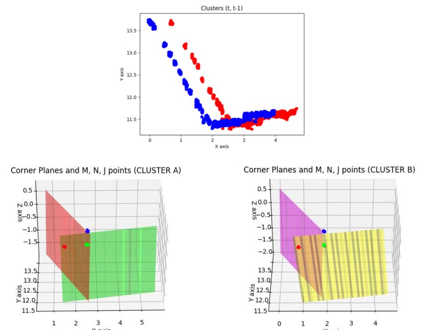
Sensors 2020, 20, 4097                                                                             2 of 30

manuevers and undertake safe stops (fail-safe), and monitoring the status of their sensors to detect
failures or malfunctions in them (fail-aware). At present, in an urban environment where there
are increasingly complex traffic elements such as multiple intersections, complex lane roundabouts,
or tunnels, a localisation system based only on GPS may pose problems. Thus, autonomous driving
will be a closer reality when LiDAR or Visual odometry systems are integrated to cover fail-operational
functions. However, fail-aware behaviour has to be integrated into the global system also.
      At present, the Global Positioning System (GPS) performs the main tasks of localisation due
to its robustness and accuracy. However, GPS coverage problems derived from structural elements
of the road (tunnels), GPS multi-path in urban areas, or failure in its operation, mean that this
technology does not meet the necessary localisation requirements in 100% of use-cases, which makes
it essential to design redundant systems based on LiDAR odometry [1], Visual odometry [2],
Inertial Navigation Systems (INS) [3], Wifi [4], or a combination of the above, including digital
maps [5]. However, LiDAR and Visual odometry systems suffer from a non-constant temporal drift,
where the characteristics of the environment and the algorithm behaviour are determinants that
improve or worsen this drift. Therefore, it is necessary to introduce, for those systems that have a
non-constant temporal drift, a fail-aware indicator to discern when these can be used.

1.2. Problem Statement
      Safe behaviour in a vehicle’s control and navigation systems depends mostly on the
redundancy and failure detections that these present. At the moment, when GPS-based localisation
fails, either temporarily or permanently, the LiDAR and Visual odometry systems can start
as redundant localisation systems, mitigating the erroneous behaviour of the GPS localisation.
Redundant localisation based on 3D mapping techniques can be applied, as well. However, this is
currently more widespread in robotic applications, as the 3D map accuracy in open environments
is decisive for localisation tasks. However, companies such as Mapillary and Here have presented
promising results for 3D map accuracy. Why is it challenging to build an accurate 3D map when
relying only on GPS localisation? It is because the GPS angular error feature of market devices is close
to 10−3 rad. This feature can place a 3D object with an error of 0.01 m when the object distance from
the sensor is 100 m.
      So, in the case of integrating redundancy into the localisation system with an odometry
alternative, a fail-aware indicator has to be integrated into the odometry system, as a consequence
of the non-constant drift error, in order for it to be used as a redundant system. The fail-aware
indicator could be based on an estimated time window that satisfies a localisation error below the
minimum requirements to planned emergency manoeuvring and placing the vehicle in a safe spot.
Several alternatives can be presented to implement the fail-aware indicator. The first is to set a fixed
time window in which the system is used. The second alternative is an adaptive time window, which is
evaluated dynamically in the continuous localisation process to find the maximum time in which the
redundant system can be used. At present, there have been no recent works focused on fail-aware
LIDAR-based odometry for autonomous vehicles.
      Therefore, it is necessary to look for an odometry process that maximises the time in exceeding the
threshold that leads the system to a failure state and, for that purpose, we propose a robust, scalable,
and precise localisation design that minimises the error in each iteration. Multiple measurement fusion
techniques from both global positioning systems and odometry systems are used to make the system
robust. Bayesian filtering guarantees an optimal fusion between the observation techniques applied in
the odometry systems and improves the localisation accuracy by integrating (mostly kinematic) models
of the vehicle’s displacement, having either three or six degrees of freedom (DoF). The LiDAR odometry
is based exclusively on the observations of the LiDAR sensor, where the emission of near-infrared
pulses and the measurement of the reflection time allows us to represent the scene with a set of
3D points, called a Point Cloud. Thus, given a temporal sequence of measurements, we obtain the
homogeneous transformation, rotation, and translation corresponding to two consecutive time instants,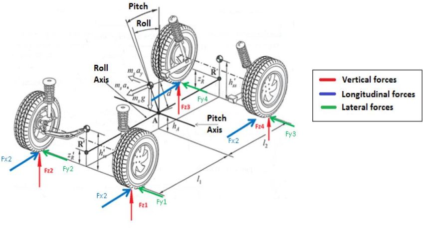
Sensors 2020, 20, 4097                                                                                                                                                       3 of 30

by applying iterative registering and optimisation methods. However, this process alone provides
incorrect homogeneous transformations if the scene presents moving objects and, so, solutions based
on feature detection must be explored in order to mitigate possible errors.

1.3. Contributions
     The factors described previously motivated us to develop an accurate LiDAR odometry system
with a fail-aware indicator ensuring its proper use as a redundant localisation system for autonomous
vehicles, as shown in Figure 1. The accurate LiDAR odometry architecture is based on robust
and scalable features. The architecture has a robust measurement topology as it integrates three
measurement algorithms, two of which are based on Iterative Closest Point (ICP) variants, and the
third one is based on non-mobile scene feature extraction and Singular Value Decomposition (SVD).
Furthermore, our work proposes a scalable architecture to integrate a fusing block, which relies
on the UKF scheme. Another factor taken into account to enhance the odometry accuracy was
to incorporate a 6-DoF motion model based on vehicle dynamics and kinematics within the filter,
where the variables of pitch and roll play a crucial impact on the precision. The proposed scalable
architecture allows us to fuse any position measurement system or integrate into the LiDAR odometry
system new measurement algorithms in a natural way. A fail-aware indicator based on the vehicle
heading error is another contribution to the state-of-the-art. The fail-aware indicator introduces, in the
system output, an estimated time to reach system malfunction, which enables other systems to take it
into consideration.

                      LiDAR odometry system

          Robust               M easure1                              M easure2                          M easure3
          feature      Variant of ICPpoint2point              Variant of ICPpoint2P lane         Features detection + SVD
                                                     z1 (t)                   z2 (t)                    z3 (t)

         Scalable                                                                                                x̂(t)
                                                              Fusion Algorithm bases on UKF
          feature                                                                                                                         Input1
                                                                                                                                                       To autonomous systems
                                                                                                                                          Redundancy
        Fail−aware                                        P̂ (t)      Fail-aware indicator based                                           Scheduler
                                                                                                                                                       where localization data
          feature                                                          on Heading Error                                                                   is needed
                                                                                                                          D−GPS           Input2
                     Secondary Localization System            Estimated time to reach the malfunction
                                                                                                                   Primary Localization
                                                                      in LiDAR pose estimation
                                                                                                                          System

      Figure 1. General diagram. The developed blocks are represented in yellow. The horizontal blue strips
      represent the main features of the odometry system. A framework where the LiDAR odometry system
      can be integrated within the autonomous driving cars topic is depicted with green blocks, such as a
      secondary localisation system.

     The global system is validated by processing KITTI odometry data set sequences and evaluating
the error committed in each of the available sequences, allowing for comparison with other
state-of-the-art techniques. The variability in the available scenes allows us to validate the fail-aware
functionality, by comparing sequences with low operating error with those with higher error,
and observing how the temporal estimation factor increases for those sequences with worse results.
     The rest of the paper is comprised of the following sections: Section 2 presents the state-of-the-art
in the areas of LiDAR odometry and vehicle motion modelling. Section 3 details the integrated
6-DoF model, while Section 4 explains the global software architecture of the work, as well as the
methodology applied to fuse the evaluated measures. Then, Section 5 describes the details of the
proposed measurement systems. Section 6 describes the methodology to make the systems fail-aware.
Section 7 describes, lists, and compares the results obtained by the developed system. Finally, Section 8
presents our conclusions and proposes a description of future work in the fields of odometry techniques,
3D mapping, and fail-aware systems.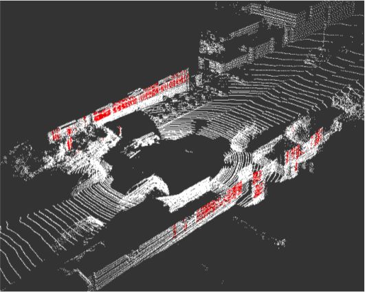
Sensors 2020, 20, 4097                                                                             4 of 30

2. Related Works
      Many contemporary conceptual systems for autonomous driving require precise localisation
systems. The geo-referenced localisation system does not usually satisfy such precision, as there are
scenarios (e.g., tunnel or forest scenarios) where the localisation provided by GPS is not correct or has
low accuracy, leading to safety issues and non-robust behaviours. For these reasons, GPS-based
localisation techniques do not satisfy all the use-cases of driverless vehicles, and it is therefore
mandatory to integrate other technologies into the final localisation system. Visual odometry
systems could be candidates for such a technology, but scenarios with few characteristics or extreme
environmental conditions lead to their non-robust performance, although considerable progress has
been made in this area, as described in [6,7]. Nevertheless, LiDAR odometry systems mitigate part of
the visual-related problems, but real-time features or accuracy in the algorithm remain issues. In the
same way as Visual Odometry, significant advances and results have been obtained, in the last few
years, in this topic.
      The general challenge in odometry is to evaluate a vehicle’s movement at all times without error,
in order to obtain zero global localisation error; however, this issue is not reachable as the odometry
measurement commits a small error in each iteration. These systems therefore have the weakness of
drift error over time due to the accumulation of iterative errors; which is a typical integral problem.
Drift error is a function of path length or elapsed time. However, these techniques have advanced in
the last few decades, due to the improvement of sensor accuracies, achieving small errors (as presented
in [8]).
      LIDAR odometry is based on the procedures of point registration and optimisation between
two consecutive frames. Many works have been inspired by these techniques, but they have
the disadvantage of not ensuring a global solution, introducing errors in their performances.
These techniques are called Iterative Closest Points (ICP), many of which have been described in [9],
where modifications affecting all phases of the ICP algorithm were analysed, from the selection and
registration of points to the minimisation approach. The most widely used are ICP point-to-point
ICPp2p [10,11] and ICP point-to-plane ICPp2p [12,13]. For example, presented a point-to-point ICP
algorithm based on two stages [10], in order to improve its exactness. Initially, a coarse registration
stage based on KD-tree is applied to solve the alignment problem. Once the first transformation
is applied, a second fine-recording stage based on KD-tree ICP is carried out, in order to solve the
convergence problem more accurately.
      Several optimisation techniques have been proposed for use when the cost function is established.
Obtaining a rigid transformation is one of the most commonly used schemes, as has been detailed
in the simplest ICP case [14], as well as in more advanced variants such as CPD [15]. This is easily
achieved by decoupling the rotation and translation, obtaining the first using algebraic tools such as
SVD (Singular Value Decomposition), while the second term is simply the mean/average translation.
Other proposals, such as LM-ICP [16] or [11], perform a Levenberg–Marquardt approach to add
robustness to the process. Finally, optimisation techniques such as gradient descent have been used in
distribution-to-distribution methods like D2D NDT [17].
      In order to increase robustness and computational performance, interest point descriptors for
point clouds have recently been proposed. General point cloud or 2D depth maps are two general
approaches to achieve this. The latter may include curvelet features, as analysed in [18], assuming the
range data is dense and a single viewpoint is used in order to capture the point cloud. However, it may
not perform accurately for a moving LiDAR—the objective of this paper. In a general point cloud
approach, Fast Point Feature Histograms (FPFH) [19] and Integral Volume Descriptors (IVD) [20] are
two feature-based global registration proposals of interest. The first one generates feature histograms,
which have demonstrated great results in vision object detection problems, using such techniques
as Histogram of Oriented Gradients (HOG), by means of computing some statistics about a point’s
neighbours relative positions and estimated surface normals. Feature histograms have shown the best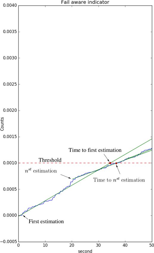
Sensors 2020, 20, 4097                                                                             5 of 30

IVD performances and surface curvature estimates. However, neither of these methods offer reliable
results in sparse point clouds and are slow to compute.
     Once one correspondence has been established, using features instead of proximity, it can be used
to initialize ICP techniques in order to improve their results. As described in previous paragraphs,
this transformation can also be found by other techniques, such as PCA or SVD, which are both
deterministic procedures. In order to obtain a transformation, three point correspondences are enough,
as is shown in the proposal we introduce in this document. However, as many outlier points are
typically present in a point cloud (such as those of vegetation), a random sample consensus (RANSAC)
approach is usually used [19]. Other approaches include techniques tailored to the specific problem,
such as the detection of structural elements of the scene [21].
     In the field of observations or measurements, there are a large number of methods for
measuring the homogeneous transformation between two moments or two point clouds. For this
reason, many filtering and fusion systems have been applied to improve the robustness of systems.
The two most widespread techniques to filter measurements are recursive filtering and batch
optimisation [22]. Recursive filtering updates the status probabilistically, using only the latest sensor
observations for status prediction and process updates. The Kalman filter and its variants mostly
represent recursive filtering techniques. However, filtering based on batch optimisation maintains
a history of observations to evaluate, on the basis of previous states, the most probable estimate of
the current instant. Both techniques may integrate kinematic and dynamic models of the system
under analysis to improve the process of estimating observations. In the field of autonomous driving,
the authors of [23] justified the importance of applying models in the solution of driving problems,
raising the need to work with complex models that correctly filter and fuse observations.
     The best odometry system described in the state-of-the-art is VLOAM [8], which is based on
Visual and LiDAR odometry. It is characterised by being a particularly robust method in the face
of an aggressive movement and the occasional lack of visual features. The method starts with a
stage of visual odometry, in order to obtain a first approximation of the movement. The final stage
is executed with LiDAR odometry. The results shown applied to a set of ad-hoc tests and the KITTI
odometry data set. The work presented as LIMO [24] also aimed to evaluate the movement of a vehicle
accurately. Stereo images with LiDAR were used to provide depth information to the features detected
by the cameras. The process includes a semantic segmentation, which is used to reject and weight
characteristic points used for odometry. The results given were related to the KITTI data set. On the
other hand, the authors of [25] presented a LiDAR odometry technique that models the projection
of the point cloud in a 2D ring structure. Over the 2D structure, an unsupervised Convolutional
Auto-Encoder (CAE-LO) system detects points of interest in the spherical ring (CAE-2D). It later
extracts characteristics from the multi-resolution voxel model using 3D CAE. It was characterised
as finding 50% more points of interest in the point cloud, improving the success rate in the cloud
comparison process. To conclude, the system described in [26] proposed a real-time laser odometry
approach, which presented small drift. The LiDAR system uses inertial data from the vehicle. The point
clouds are captured in motion, but are compensated with a novel sweep correction algorithm based on
two consecutive laser scans and a local map.
     To the best of our knowledge, there have been no recent works focused on fail-aware LiDAR-based
odometry for autonomous vehicles.

3. Kinematic and Dynamic Vehicle Model
     Filters usually leverage mathematical models to better approximate state transitions. In the field
of vehicle modelling, there are two ways to study the movement of a vehicle: with kinematic or
dynamic models. In the field of kinematic vehicle modelling, one of the most-used models is the
bicycle model, due to its ease of understanding and simplicity. This model requires knowledge of the
slide angle (β) as well as the front wheel angle (δ) parameters. These variables are usually measured
by dedicated car systems.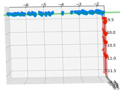
Sensors 2020, 20, 4097                                                                                           6 of 30

     In this work, the variables β and δ are not registered in the data set, so the paper proposes
an approach based on a dynamic model to evaluate them. The method proposed can be used as a
redundancy system, replacing dedicated car systems. The technique relies on the application of LiDAR
odometry and the application of vehicle dynamics models where linear and angular forces are taken
into account and the variables β and δ are assessed during the car’s movement. Figure 2 depicts the
actuated forces in the x and y car axes, as well as the slip angle and the front-wheel angle. Given these
variables, the bicycle model is applied to predict the car’s movement.

                   yw

                                                                               y                    x
                                                                                                        δ
                                                                                    R
                                                                               LiDA
                                                                                       β         F yf
                                                                                           V
                                                                  F yr
                                                   δ
                                              x

                                                   f
                                                  Fy
                                 AR
                                   β
                             LiD
                         y

                                          V

                                      ψ

                                                                                                            xw
                             r
                         Fy

      Figure 2. Vehicle representation by bicycle model. Using the vehicle reference system, our LiDAR-based
      odometry process assesses the vehicle forces between two instants of time, allowing for estimation of
      the β and δ variables.

     From a technical perspective, the variables β and δ are evaluated using Equations (1) and (2).
Equation (1) represents Newton’s second law, applied on the car’s transverse axis in a linear form and
on the car’s z-axis in an angular form.

                                              Translational :    m(ÿ + ψ̇v x ) = Fy f + Fyr
                                                                                             ,                      (1)
                                                Angular :          Iz ψ̈ = l f Fy f − lr Fyr

where m is the mass of the vehicle, v x is the projection of the speed car vector V on its longitudinal
axis x, Fy f and Fyr are the lateral forces produced on the front and rear wheel, Iz is the inertia moment
of the vehicle concerning to the z-axis, and l f and lr are the distances from the centre of masses of the
front and rear wheels, respectively.
      The lateral forces Fy f and Fyr are, in turn, functions of characteristic tyre parameters, cornering
stiffnesses Cα f and Cαr , the vehicle chassis configuration l f and lr , the linear and angular travel speed
to which the vehicle is subjected to v x , ψ̇, the slip angle β, and the turning angle of the front wheel δ,
as shown in Equation (2):
                                                                                  l f ψ̇
                                                          Fy f = Cα f (δ − β −     vx )
                                                                               lr ψ̇
                                                                                                                    (2)
                                                            Fyr = Cαr (− β +    vx )

     Therefore, knowing the above vehicle parameters and assessing the variables ÿ, v x , ψ̈, and ψ̇ from
the LiDAR odometry displacement, with the method proposed in this work (see Figure 3), the variables
β and δ can be derived by solving the two-equation system shown in Equation (1).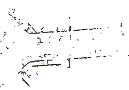
Sensors 2020, 20, 4097                                                                                                                                   7 of 30

                                                                                                                      1)
                                                                                                             β (t +
                                                                                                                                x                   1)
                                                                                                     y
                                                                                                                                           δ (t +

                                                                               t)
                                                                             δ(
                   yw                                                                                                        F yf

                                                                      x
                                                                                                                        )
                                                                                             LiDA
                                                                                                 R             V(t+1

                                                          t)
                                                      β(

                                                                          yf
                                                                                      F yr

                                                                         F
                                                                                                                      ψ(t)−ψ(t−1)
                                                                                                     ψ̇(t) =

                                                                   t)
                                                y

                                                                 V(
                                                                                                                       Todometry
                                                               ψ(t)
                                                                ∆ytt−1                                                ψ̇(t)−ψ̇(t−1)
                                           1)                                                        ψ̈(t) =

                                                      R
                                                                                                                        Todometry
                                      δ (t −

                                                    DA
                                                Li
                                                yr
                                                F
                                  x

                                                                                               ∆xt−1
                                                                                  vx (t) =        t
                                      Fyf

                                                    ∆xt−1                                     Todometry
                     1)

                                                      t
                   β (t −

                                                                                              ∆ytt−1
                                                                                  ẏ(t) =
                                      )
                                   V(t−1

                                                                                             Todometry

                                  ψ(t − 1)                                                   vx (t)−vx (t−1)
                   y

                                                                                  ẍ(t) =       Todometry
                            R
                          LiDA

                                                                                             ẏ(t)−ẏ(t−1)
                                                                                  ÿ(t) =      Todometry
                            Fyr

                                                                                                                                      xw

                             Figure 3. Evaluation of variables ÿ, v x , ψ̈, ψ̇ with LiDAR odometry.

     Finally, the variables β and δ are used in the kinematic bicycle model defined by Equation (3) to
obtain the speeds [ Ẋ, Ẏ, ψ̇] which, in turn, are used to output the predicted vehicle pose at time (t + 1).

                                                                  Ẋ = V cos(ψ + β)
                                                                  Ẏ = V sin(ψ + β)                      .                                                  (3)
                                                                 V cos( β)
                                                      ψ̇ =        l f +lr (tan( δ f ) − tan( δr ))

     However, the model mentioned above evaluates the vehicle’s motion only in 3-DoF, while the
LiDAR odometry gives us full 6-DoF displacement. Therefore, to assess the remaining 3-DoF,
we propose to use another dynamic model based on the behaviour of the shock absorbers and
the position of the vehicle’s mechanical pitch (θ) and roll (α) axes; see Figure 4. Appling this second
dynamical model, we can predict the car’s movement in terms of its 6-DoF.

      Figure 4. Detail of forces and moments applied to the vehicle. The distance d represented is broken
      down into d picth and droll , concerning the pitch and roll axes of rotation, respectively. The figure
      references [27].
Sensors 2020, 20, 4097                                                                                            8 of 30

     From a technical perspective, in order to evaluate these variables, we need to take into
consideration the angular movement caused in the pitch and the roll axes.
     First, regarding the pitch axis, the movement is due to the longitudinal acceleration suffered
in the chassis, producing front and rear torsion on the springs and shock absorbers of the vehicle.
Given the parameters D pitch and K pitch , which represent the distance between the centre of the pitch
axis with respect to the centre of mass of the vehicle and the characteristics of the spring together with
the shock absorber, respectively, Equation (4) defines the dynamics of the pitch angle, which represents
the sum of the moments of forces applied to the pitch axis. The angular acceleration suffered by the
vehicle chassis for the pitch axis is obtained by Equation (5), while the variables ẍ, θ, and θ̇ are found
in the LiDAR odometry process.

                          ( Iy + m d2pitch )θ̈ − m d pitch ẍ + (K pitch + m g d pitch )θ + D pitch θ̇ = 0           (4)

                                            −m d pitch ẍ + (K pitch + m g d pitch )θ + D pitch θ̇
                                   θ̈ = −                                                                            (5)
                                                                  Iy + m d2pitch

where
                                                             dshock f l 2f + dshock r lr2
                                                D pitch =
                                                                           2                                         (6)
                                                             Kspring f l 2f + Kspring r lr2
                                                K pitch =
                                                                            2
     With the pitch acceleration and applying Equation (7), representing uniformly accelerated motion,
the pitch of the vehicle can be predicted at time (t + 1).

                                                         1
                                              θe(t + 1) = θ̈ (t)dt2 + θ̇ (t)dt + θ (t)                               (7)
                                                         2
     On the other hand, the angular movement caused on the roll axis is due to the lateral acceleration
or lateral dynamics suffered in the chassis. The parameter droll is the distance between the roll
axis centre and the centre of mass of the vehicle, and mainly depends on the geometry of the
suspension. The lateral forces multiplied by the distance droll generate an angular momentum, which is
compensated for by the springs (Kroll f , Krollr ) and lateral shock absorbers of the vehicle (Droll f , Drollr ),
minimising the roll displacement suffered in the chassis. Equation (8) defines the movement dynamics
of the roll angle, which represents the movement compensation effect with the sum of moments of
forces applied on the axle.

              ( Ix + m d2roll )α̈ − m droll ÿ + (Kroll f + Krollr + m g droll )α + ( Droll f + Drollr )α̇ = 0,      (8)

                                  −m droll ÿ + (Kroll f + Krollr + m g droll )α + ( Droll f + Drollr )α̇
                         α̈ = −                                                                               ,      (9)
                                                                   Ix + m d2roll
where

                                  Droll f = dshock f t2f                        Drollr = dshock r t2r
                                              Kspring f t2f ,                               Kspring r t2r .        (10)
                                  Kroll f =                                     Krollr =
                                                    2                                            2

     Given the roll acceleration and applying the uniformly accelerated motion Equation (11), the roll
of the vehicle can be predicted at time (t + 1):

                                                             1
                                              e
                                              α ( t + 1) =     α̈(t)dt2 + α̇(t)dt + α(t).                          (11)
                                                             2
Sensors 2020, 20, 4097 9 of 30
Finally, to complete the 6-DoF model parameterisation, we need to consider the vertical
displacement of the vehicle, which is related to the angular movements of pitch and roll. Equation (12)
represents the movement of the centre of masses concerning the vehicle z-axis, where COGz is the
height of the vehicle’s centre of gravity at resting state:
z(t + 1) = COGz + d pitch (cos(θe(t + 1)) − 1) + droll (cos(e
e α(t + 1)) − 1) (12)
Table 1 lists the parameters and values used in the 6-DoF model. The values correspond to a
Volkswagen Passat B6, and were found in the associated technical specs.
Table 1. Model parameters (chassis, tires, and suspension).
Name Value
m = 1750 kg Vehicle mass
N
Kspring f = 30,800 m Front suspension spring stiffness
N
Kspring r = 28,900 m Rear suspension spring stiffness
Dshock f = 4500 Nsm Front suspension shock absorber damping coefficient
Dshock r = 3500 Nsm Rear suspension shock absorber damping coefficient
droll = 0.1 m Vertical distance between COG and roll axis
d pitch = 0.25 m Vertical distance between COG and pitch axis
Ix = 540 kg m2 Vehicle’s moment of inertia, with respect to the x axis
Iy = 2398 kg m2 Vehicle’s moment of inertia, with respect to the y axis
Iz = 2875 kg m2 Vehicle’s moment of inertia, with respect to the z axis
COGz = 0.543 m COG height from the ground
l f = 1.07 m Distance between COG and front axle
lr = 1.6 m Distance between COG and rear axle
t f = 1.5 m Front axle track width
tr = 1.5 m Rear axle track width
To deal with the imperfections of the kinematic model, we compared the output of the proposed
6-DoF model with the ground truth available in the KITTI odometry data set. The analysis was applied
to all available sequences, in order to measure the uncertainty model in the best way.
By evaluating the pose differences (see Figure 5), the probability density function of the 6-DoF
model was calculated, as well as the covariance matrix expressed in Equation (13).
2
σxx 2
σyx 2
σzx 2
σφx 2
σθx 2
σψx
2 2 2 2 2 2
σxy σyy σzy σφy σθy σψy
σ2 2 2 2 2 2
xz σyz σzz σφz σθz σψz
Q= 2 2 2 2 2 2 , (13)
σxφ σyφ σzφ σφφ σθφ σψφ
σ2 2
σyθ 2
σzθ 2
σφθ 2
σθθ 2
σψθ
xθ
2
σxψ 2
σyψ 2
σzψ 2
σφψ 2
σθψ 2
σψψ
where σxx = 0.0485 m, σyy = 0.0435 m, σzz = 0.121 m, σφφ = 0.1456 rad, σθθ = 0.1456 rad, σψψ = 0.0044 rad,
and the error covariance between variables has a zero value.Sensors 2020, 20, 4097 10 of 30
Figure 5. Probabilistic error distribution representation for each vehicle output variable.
4. Vehicle Pose Estimation System
This section details the architecture implemented to estimate the vehicle’s attitude, by integrating
the dynamic and kinematic model described in Section 3 and fusing the LiDAR-based measurement
system described in Section 5. Several works have analysed the response of two of the most well-known
filters for non-linear models, the Extended Kalman Filter (EKF) and the Unscented Kalman Filter
(UKF), where the results were generally in favour of the UKF. For instance, in [28], the behaviour
of both filters was compared to estimate the position and orientation of a mobile robot. Real-life
experiments showed that UKF has better results in terms of localisation accuracy and consistency of
estimation. The proposed architecture therefore integrates an Unscented Kalman Filter [29], which is
divided into two stages: prediction and update (as shown in Figure 6).
Input Data − LiDAR Point Cloud
Sweep correction of Point Cloud
with xe(t + 1)
Fusion Process of 3 Measurements
z(t + 1)
Update
Predicted (t+1)
t+1: x
b(t + 1)
behaviour
+
e(t + 1)
t :x
Predition t: x
b(t)
6DOF Dynamic Model
Figure 6. Unscented Kalman Filter (UKF) architecture. The prediction phase relies on the 6-DoF
motion model detailed in the previous section. The update phase uses three consecutive LiDAR-based
measurements to fuse and estimate the vehicle state.Sensors 2020, 20, 4097 11 of 30
The prediction phase manages the 6-DoF dynamic model described in the previous section to
predict the system’s state at time (t + 1). Along with the definition of the model, the model noise
covariance matrix Q must be associated, as defined by the standard deviations evaluated above.
The model noise covariance matrix is only defined in its main diagonal and is constant over time.
Equation (14) represents the prediction phase of the filter.
x(t + 1) = Ab
e x(t) + Q, (14)
where x is the 6-DoF state vector, as shown in Equation (15), and A matrix represents the developed
dynamic model. h i
x0 (t) = x (t) y(t) z(t) α(t) θ (t) ψ(t) . (15)
In the filter update phase, the LiDAR odometry output is estimated. The estimated state vector,
x(t + 1), is represented, in terms of the state variables, by Equation (16). The 6 × 6 matrix C is defined
b
with the identity matrix, as the vectors z(t + 1) and b x(t + 1) contain the same measurement units.
Finally, the matrix R is the covariance error matrix of the measurement, which is updated every
odometry period in the measurement and fusion process, as explained in Section 5. The matrix R is
only defined in its main diagonal, representing the uncertainty of each of the magnitudes measured in
the process.
z(t + 1) = Cb x(t + 1) + R. (16)
LiDAR Sweep Correction
To use the LiDAR data in the update phase of the UKF, it is recommended to perform a
so-called sweep correction of the raw data. The sweep correction phase is due to the nature of
most LiDAR devices, which are composed of a series of laser emitters mounted on a spinning head
(e.g., the Velodyne HDL-64E). The sweep correction process becomes crucial when the sensor is
mounted on a moving vehicle, as the sensor spin requires a time span close to approximately 100 ms,
as in the case of the Velodyne HDL-64E. The sweep correction process consists of assigning two poses
for each sensor output and interpolates the poses with constant angular speed for all the LiDAR
beams. These poses are commonly associated with the beginning and the end of the sweep. Thus,
the initial pose is equal to the last filter estimation b
x and the final pose is equal to the filter prediction
x(t + 1) to carry out the interpolation. The whole point cloud is corrected with the interpolated poses
e
evaluated, solving the scene deformation issue when the LiDAR sensor is mounted on a moving
platform. Figure 7a shows the key points on the sweep correction process.
Regarding the correction method, the authors in [30,31] proposed a point cloud correction
procedure based on GPS data. The process requires synchronisation between each GPS and LiDAR
output, a complex task when the GPS introduces small delays in its measurement. For this reason,
in our case, the GPS data is replaced with the filter prediction to apply the sweep correction process.
Figure 7b shows the same point cloud with and without sweep correction, captured in a roundabout
with low angular speed vehicle movement. It can be seen that there is significant distortion concerning
reality, as the difference of shapes between clouds is substantial, leading to errors of one meter in many
of the scene elements. We can claim that the motion model accuracy is a determinant for the sweep
correction process, as it improves the odometry results (as we depict in Section 7).Sensors 2020, 20, 4097 12 of 30
x
LiDAR position:
y
2π − rad
Asigned pose:
e(t + 1)
x
x New LiDAR Point Cloud
Asigned pose:
y
b(t)
x
LiDAR position:
0+ rad (b)
(a)
Figure 7. Sweep correction process in odometry: (a) the assignment of two poses to the point cloud
when the vehicle is moving; and (b) raw (blue) and corrected measurements (red). An important
difference between the measurement results of both point clouds is exposed, the correction being
decisive for the result of the following stages.
5. Measurements Algorithms and Data Fusion
Three measurement methodologies based on LiDAR raw-data were developed to provide an
accurate and robust algorithm. Two of them are based on ICP techniques, and another one relies on
feature extraction and SVD. A 6-DoF measure z(t) is the output of this process, after the fusion process
is finished.
5.1. Multiplex General ICP
Using the ICP algorithm for the development of LiDAR odometry systems is very common,
where the two most used versions are the Point-to-Point and Point-to-Plane schemes. Adaptations of
both algorithms have been developed for our approach. For the first measurement system developed,
we propose the use of the ICP point-to-point algorithm, which is based on aligning two partially
overlapping point clouds to find the homogeneous transformation matrix ( R, t) in order to align the
two point clouds. The ICP used is based on minimising the cost function defined by the mean square
error of the distances between points in both clouds, as expressed in Equation (17). The point cloud
registration follows the criterion of the nearest neighbour distance between clouds.
Np
1
min(error ( R, T )) = min(
R,T R,T Np ∑ k pi − (qi R + T )k), (17)
1
where pi represents the set of points that defines the cloud captured at a time instant (t − 1),
qi represents the set of points that define the cloud captured at a time instant t, Np is the number of
points considered in the minimisation process, R is the resulting rotation matrix, and T is the resulting
translation matrix.
The ICP technique, as with many other gradient descent methods, can become stuck at a local
minimum instead of the global minimum, causing measurement errors. The possibility of finding
moving objects or a lack of features in the scene are some of the reasons why the ICP algorithm
provides local minimum solutions. For this reason, an algorithm that computes the multiplex ICP
algorithm for a set of distributed seeds was implemented. The selected seed, such as the ICP starting
point, is evaluated with the Merwe Sigma Points method [32,33]. The error covariance matrix predicted
by the filter Pe(t + 1) and the predicted state vector xe(t + 1) are the input to assess the eight seeds
needed. Figure 8 shows an example of seed distribution in the plane ( x, y) for a time instant (t).Sensors 2020, 20, 4097 13 of 30
se e d
8
+ 1)
xe(t se e d
1
1)
e (t +
P
se e d
2
t)
xb(
Figure 8. Sharing of Iterative Closest Points (ICP) initial conditions applying the Sigma Point techniques
in the limits marked by Pe(t + 1).
After evaluating the eight measures, the one with the best mean square error in the ICP process is
selected. After the evaluation of two sequences of the KITTI data set, a decrease of error close to 9.5%
was discerned, this being the determining reason why eight seeds were selected. However, the increase
in computation time could be a disadvantage.
5.2. Normal Filtering ICP
For the design of a robust system, it is not enough to integrate only one measurement technique,
as it may fail due to multiple factors. Therefore, a second measurement method based on ICP
point-to-plane was developed to improve the robustness of the system, as it implies a lower
computation time than the one above. In [34], the results with the point-to-plane method were
more precise than those with the point-to-point method, improving the precision of the measurement.
The cost function to be minimised in the point-to-plane process is as follows (18):
Np
1
∑
p
min(error ( R, T )) = min( ( pi − (qi R + T )) · ni ), (18)
R,T R,T Np 1
where R and T are the rotation and translation matrices, respectively, Np is the number of points used
p
to optimize, pi represents the source cloud, qi represents the target cloud, and ni represents the normal
unit vector of a point in the target cloud. The point-to-plane technique is based on a weighting to
register cloud points in the minimisation process, where cos(θ ) from the vectorial product is the weight
p
given in the process and θ is the angle between the unit normal vector ni and the vector resulting from
the operation ( pi − (qi R + T )). Therefore, the smaller the angle θ is, the higher the contribution in the
p
added term of this register point is. So, the normal unit vector ni can be understood as rejecting or
decreasing the impact over the added term of its register points when the alignment with the unitary
vector is not right. The approach in this paper does not include all the points registered, as a filter
process is carried out. The heading of the vehicle is the criteria to implement the filtering process.
Thus, only those points that have a normal vector within the range ψ ev ± e
σψψ rad are considered in
e
the added term, where ψv represents the heading of the predicted vehicle and e σψψ represents theSensors 2020, 20, 4097 14 of 30
uncertainty predicted from the error covariance matrix. Equation (19) formulates the criteria applied
in the minimisation to filter out points:
N p
minJ ( R, T ) = min( N1p ∑1 p ( pi − (qi R + T )) · ni )
R,T
s.t. (19)
p ev ± e
ni > ψ σψψ
p ev ± e
ni > ψ σψψ + π
Points that are not aligned with the longitudinal and transverse directions of the vehicle are
eliminated from the process, improving the calculation time of this process as well as the accuracy of
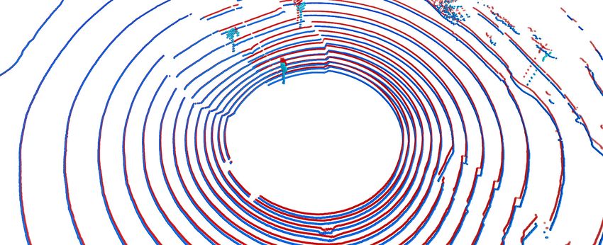
the measurement. Figure 9 represents an ICP iteration of the described technique, where the results
achieved by RMSE are 20% better than if all the points of the cloud are considered.
z
pi
npi
pi − (qi R − t)θ
qi y
x
(b)
(a)
Figure 9. ICP process based on normals: (a) Graphical representation of the cost function with the
p
normal unit vector ni used to enter constraints in ICP; and (b) ICP output result applying constraints
of normals. The figure shows the overlap of two consecutive clouds.
5.3. SVD Cornering Algorithm
The two previous systems of measurement are ICP-based techniques, where there is no known
data association between the points of two consecutive point clouds. However, the third proposed
algorithm uses synthetic points generated by the algorithm and the data association of the synthetic
point between point clouds to evaluate the odometry step. An algorithm for extracting the
characteristics within the point clouds is developed to assess the synthetic points. The corners
built up with the intersection between planes are the features explored. The SVD algorithm uses the
corners detected in consecutive instants to determine the odometry between point clouds. The new
odometry complements the two previous measurements. The SVD algorithm is accurate and has
low computational load, although the computation time increases in the detection and feature
extraction steps.
5.3.1. Synthetic Point Evaluation
Plane Extraction
It is easy for humans to identify flat objects in an urban environment; for instance, building walls.
However, identifying vertical planes in a point cloud with an algorithm is more complex. The algorithm
identifies points that, at random heights, fit the same projection on the plane ( x, y). Therefore,
the number of repetitions that each beam of the LiDAR presents on the plane ( x, y) is recorded. If the
number of repetitions of the project exceeds the threshold of 20 counts, the points belong to a vertical
plane. Figure 10 shows detected points that belong to vertical planes, although the planes in many
cases are not segmented.Sensors 2020, 20, 4097 15 of 30
(a) (b)
Figure 10. Intermediate results of sequence 00, frame 482: (a) Input cloud to the plane detection
algorithm; and (b) points detected on candidate planes.
Clustering
Clustering techniques are then used to group the previously selected points into sets of intersecting
planes. Among those listed in the state-of-the-art, those that do not imply knowing the number of
clusters to be segmented were considered valid, as it is not known a priori. Analysing the clustering
results provided by the Sklearn library, DBSCAN was the one that obtained the best results, as it
does not make mistakes when grouping points of the same plane in different clusters. In order to
provide satisfactory results, the proposed configuration of the DBSCAN clustering algorithm sets the
maximum distance between two neighbouring points (0.7) and the minimum number of samples
between neighbours (50). The algorithm identifies solid structure corners, such as building walls,
such that clusters associated to non-relevant structures are eliminated. For this purpose, clusters
sized smaller than 300 points were filtered, eliminating noise produced by vegetation or pedestrians.
Figure 11 represents the cluster segmentation of the point cloud depicted in Figure 10, where only the
walls of buildings, street lights, or traffic signs are segmented as characteristic elements of the scene.
(a) (b)
Figure 11. Results of clustering, sequence 00 of the KITTI odometry data set: (a) Frame 0,
and (b) Frame 482.
Corner Detection and Parameters Extraction
In addition, to eliminate straight walls, cylindrical points, or a variety of shapes that are not valid
for the development of the algorithm, clusters that do not contain two vertical intersected planes are
discarded, as shown in Figure 11. Thus, two intersecting planes are searched for in the cluster that
satisfies the condition of forming an angle between both higher than 45◦ and less than 135◦ . Using the
RANSAC algorithm on the complete set of points of the cluster, indicating that it selects a quarter of the
total points and fixing the maximum number of iterations as 500 iterations, the algorithm returns the
equation of a possible intersected plane in the cluster. Applying RANSAC again to the outlier points
resulting from the first process and with the same configuration parameters, a second intersected planeSensors 2020, 20, 4097 16 of 30
in the cluster is achieved, as shown in Figure 12. If the angle formed between the two intersected
planes fulfils the previous conditions, the intersection line of both planes is evaluated to obtain the
synthetic points that define the evaluated corner.
(a) (b)
Figure 12. Results of extraction of intersected planes: (a) Input data to cluster planes; and (b) detection
results of two intersecting planes, represented in red and green.
Synthetic Points Evaluation
At this point, the objective is to generate three points that characterize the corners of the scene;
these points are denoted as synthetic points. The synthetic points are obtained from the intersection
line equation derived from the two intersecting planes. Figure 13a shows the criterion followed to
evaluate three synthetic points for each of the detected corners. Two of the synthetic points, ( M, J ),
belong to the intersection line and are located at a distance of 0.5 m. The third synthetic point, N, meets
the criterion of being at 1 m of point separation from M with a value of z = 0. The process identifies,
as the reference plane, the one that has the lowest longitudinal plane direction evaluated within the
global co-ordinate system. Figure 13b shows the points ( M, J, N ) evaluated in two consecutive instants
of time. In this situation, the SVD algorithm can be applied to assess the homogenous transform
between two consecutive point clouds when the synthetic points data association is known.
z
1 Plan
e e2
Plan
J y
0.5m
M
1m N
x
(a)
(b)
Figure 13. Evaluation of synthetic points: (a) Nomenclature and position of calculated synthetic points;
and (b) result of synthetic points detection in real clusters of two consecutive time instants.Sensors 2020, 20, 4097 17 of 30
5.3.2. SVD
Before applying the SVD, the registration of the extracted points of the corners between
two consecutive instants need to be done. So, let us suppose that, for an instant t, there is a set
of corners X = x1 , x2 , x3 , ..., xn where x1 = ( M1 , N1 , J1 ) and, for another instant t + 1, there is another
set of corners Y = y1 , y2 , y3 , ....ym where y1 = ( M1 , N1 , J1 ). Then, to register both sets, the Euclidean
distance of points M is used. Only those corners that show a minimum distance less than 0.5 m are
data associated. The non-data associated corners are removed.
Once the data association of synthetic corners is fulfilled, the objective is to find the homogeneous
transformation between two consecutive scenes. Therefore, SVD minimises the distance error between
synthetic points, first by eliminating the translation of both sets to exclude the unknown translation
and then by solving the Procustes orthogonal problem to obtain the rotation matrix ( R). Finally,
it undoes the translation to obtain the translation matrix ( T ). Equation (20), described in more detail
in [35], shows the mathematical expressions applied in the SVD algorithm to obtain the homogeneous
transformation matrix between two sets of synthetic corners at consecutive time instants:
X 0 = xi − µ x = xi 0
Y 0 = yi − µ y = yi 0
Np
W = ∑ i =1 x i 0 y i 0 T
. (20)
W = U ∑ VT
R = UV T
t = µ x − Rµy
The SVD odometry measure zSVD is fused with the other measurements, but the factor related
to the uncertainty must be added to the SVD homogeneous transformation ∆ PoseSVD . Therefore,
Equation (21) defines the SVD measure added to the ∆ PoseSVD , the UKF estimated state vector xe(t),
and the uncertainty factor RSVD . The uncertainty represents the noise covariance matrix of the SVD
measurement and RSVD is calculated with the RMSE returned by the RANSAC process applied within
the method. The decision taken is a consequence of distinguishing a direct relationship between RSVD
and how well the intersection planes are fitted over the points of the cluster.
zSVD = xe(t) + ∆ PoseSVD + RSVD . (21)
Figures 14 and 15 depict a successful scenario where SVD odometry is evaluated. The colour code
used in the figure is: green (M points), blue (J points), and orange (N points).
Figure 14. Odometry results with Singular Value Decomposition (SVD): Input cluster to extract
synthetic points.Sensors 2020, 20, 4097 18 of 30
(a) (b)
Figure 15. Odometry results with SVD: (a) Representation of the synthetic points extracted from the
previous clusters. A translation and rotation between them is shown; and (b) synthetic points are
overlapped when applying the rotation and translation calculated by SVD.
5.4. Fusion Algorithm
An essential attribute in the design of a robust system is the redundancy. For the proposed work,
three measurement techniques based on LiDAR were developed. Therefore, it is necessary to integrate
sensor fusion techniques that allow for selecting and evaluating the optimal measurement from
an input set to the solution. Figure 16a shows an architecture where the filter outputs—that is,
the estimated state vectors—are fused. The main architecture characteristic is that multiplex filters have
to be integrated into the solution. Figure 16b shows an architecture that fuses a set of measurements
and then filters the fused measurement. For this architecture design, only blocks have to be designed,
improving its simplicity. In this second case, all the measurements must represent the same magnitude
to be measured. In [36], a system that merges the data from multiple sensors using the second approach
was presented. The proposed fusion system implements this sensor fusion architecture, in which the
resulting measurement vector comprises the 6-DoF of the vehicle.
z1 x̂1 z1
UKF
z2 x̂2 z2
UKF
x̂ z
Fuser Fuser UKF x̂
x̂n
zn UKF zn
(a) (b)
Figure 16. Block diagram for two fusion philosophies: (a) Merging of the estimated state vector,
which requires a filtering stage for each measure to be merged; and (b) merging of observations under
a given criterion and subsequent filtering.
The proposed sensor fusion consists of assigning a weight to each of the measurements.
The weights are evaluated considering the distance (x, y) between the filter prediction and the
LiDAR-based measurements. Therefore, Equation (22) defines the weighting function. The assigned
weight varies between 0 and 1 when the measurement is within the uncertainty ellipse. The assigned
weight is 0 when the measurement is outside the uncertainty ellipse, as shown in Figure 17.Sensors 2020, 20, 4097 19 of 30
The predicted error covariance matrix Pe(t + 1) defines the uncertainty ellipse. The weighted mean
value is the fused measurement, as detailed in Equation (23). In the same way, the uncertainty
associated with the fused measure is weighted with the partial measure weight. Thus, the sensor
fusion output is a 6-DoF measure with an associated uncertainty matrix R.
r
I f (z x − xex (t+1))2
+
zy − xey (t+1)
≤1 ⇒ w= (z x − xex (t+1))2
+
zy − xey (t+1)
−1
2
σxx 2
σyy 2
σxx 2
σyy
(22)
I f (z x − x x (t+1))2
e zy − xey (t+1)
2
σxx
+ 2
σyy
>1 ⇒ w=0
(z1 − xe(t + 1))w1 + (z2 − xe(t + 1))w2 + (z3 − xe(t + 1))w3
z = xe + (23)
w1 + w2 + w3
Fusing the set of available measurements provides the system with robustness and scalability.
It is robust because, if any of the developed measurements fail, the system can continue to operate
normally, and it is scalable as other measurement systems are easy to integrate using the weighting
philosophy described above. Furthermore, the integrated measurement systems can be based on any
of the available technologies, not only LiDAR. As the number of measurements increases, the result
achieved should improve, considering the principles of Bayesian statistics.
yw
z2 = 0
w2
1 )
1) t+
xe(t
+ e xx(
σ
1 )
w3 y(
t+
ey
σ
z3
z1
w1
Model trajectory output
(t)
t) σe xx
xe(
z2 (t)
σe yy
2 w3
w z3
z1
w1
xw
Figure 17. Representation of predicted ellipses of uncertainty and weight allocation to each measure to
be applied in fusion.
6. Fail-Aware Odometry System
The estimated time window evaluated by the fail-aware indicator is recalculated for each instant
of time, allowing the trajectory planner system to manage an emergency manoeuvre in the best way.
In practice, most odometry systems do not implement this kind of indicator. Instead, our approach
proposes the use of the evaluated heading error, as the heading error magnitude is critical for the
localisation error. Thus, a small heading error at time t produces a huge localisation error at time t + N
if the vehicle has moved hundreds of meters away. For example, a heading error equal to 10−3 rad at
t introduces a localisation error of 0.01 cm at t + N if the vehicle moves only 100 m. This behaviour
motivates us to use the heading error to develop the fail-aware indicator.
The estimated heading error has a significant dependence on the localisation accuracy.
The developed fail-aware algorithm is composed of two parts: a function to evaluate the fail-aware
indicator and a failure threshold, which is fixed as 0.001. This threshold value was chosen by using
heuristic rules and analysing the system behaviour in sequences 00 and 03 of the KITTI odometry data
set. We evaluated the fail-aware indicator (η) on each odometry execution period, in order to estimateSensors 2020, 20, 4097 20 of 30
the remaining time to overtake the fixed malfunction threshold. Equation (24) defines the fail-aware
indicator, where σψψ is the estimated heading standard deviation and σψψ is identified as the variable
most correlated with the localisation error; once again, regarding the error results in sequences 00
and 03.
For this reason, σψψ is useful to evaluate the fail-aware indicator. The second derivative of σψψ is
used, representing the heading error acceleration, so how fast or slow this magnitude changes is used
as a determinant to find the estimated time of reaching the malfunction threshold. If the acceleration
of σψψ is low, the estimated time window is large and the trajectory planner has more time to perform
an emergency manoeuvre. On the other hand, if the acceleration of σψψ is high, the estimated time
window be decisive with respect to stopping the car safely in a short time.
The acceleration of σψψ can be positive or negative, but the main idea is to accumulate the absolute
value for all the odometry interactions, in order to have an indicator that allows us to know the
estimated time window. The limit time t1 in the addition term represents when the LiDAR odometry
system starts to work as a redundant system for localisation tasks. In this way, the speed η is calculated
as the difference between two consecutive η values, in order to assess the time to reach the malfunction
threshold. Figure 18 shows the behaviour of the fail-aware algorithm. In all the use-case studies,
the Euclidean error [ x, y] is approximated as 0.6 m when the malfunction threshold is exceeded.
The Euclidean XY error depicted in the image is calculated by comparing the LiDAR localisation
and the available GT. The fail-aware algorithm provides a continuous diagnostic value of the LiDAR
system, allowing for the development of more robust and safe autonomous vehicles.
∞
d2
η= ∑ dt2
b
σψψ (24)
t=t1
(a) (b) (c)
Figure 18. Fail-aware process. Sequence results 03. (a) Evolution of the signal standard deviation of ψ b
estimated by the filter (σψψ ). (b) Representation of the failure threshold (red) and fail-aware indicator
η (blue). The green lines represent the equation to evaluate the time window to reach the failure
threshold. (c) Euclidean [ x, y] error compared with the ground truth (GT) of the data set.You can also read