Possible Interstellar meteoroids detected by the Canadian Meteor Orbit Radar
←
→
Page content transcription
If your browser does not render page correctly, please read the page content below
Possible Interstellar meteoroids detected by the
                                                              Canadian Meteor Orbit Radar

                                                             Mark Froncisza , Peter Browna,b,1 , Robert J. Werykc
arXiv:2005.10896v1 [astro-ph.EP] 21 May 2020

                                                  a Dept.  of Physics and Astronomy, University of Western Ontario, London, Ontario,
                                                                                    Canada N6A 3K7
                                                b Centre for Planetary Science and Exploration, University of Western Ontario, London,

                                                                               Ontario, Canada N6A 5B7
                                                       c Institute for Astronomy, University of Hawaii, Honolulu, HI, 96822, USA

                                               Abstract

                                                  We examine meteoroid orbits recorded by the Canadian Meteor Orbit Radar
                                               (CMOR) from 2012-2019, consisting of just over 11 million orbits in a search for
                                               potential interstellar meteoroids. Our 7.5 year survey consists of an integrated
                                               time-area product of ∼ 7× 10⁶ km2 hours. Selecting just over 160000 six sta-
                                               tion meteor echoes having the highest measured velocity accuracy from within
                                               our sample, we found five candidate interstellar events. These five potential
                                               interstellar meteoroids were found to be hyperbolic at the 2σ-level using only
                                               their raw measured speed. Applying a new atmospheric deceleration correction
                                               algorithm developed for CMOR, we show that all five candidate events were
                                               likely hyperbolic at better than 3σ, the most significant being a 3.7σ detection.
                                               Assuming all five detections are true interstellar meteoroids, we estimate the in-
                                               terstellar meteoroid flux at Earth to be at least 6.6 × 10⁻⁷ meteoroids/km2 /hr
                                               appropriate to a mass of 2 × 10⁻⁷ kg.
                                                  Using estimated measurement uncertainties directly extracted from CMOR
                                               data, we simulated CMOR’s ability to detect a hypothetical ‘Oumuamua - asso-
                                               ciated hyperbolic meteoroid stream. Such a stream was found to be significant
                                               at the 1.8σ level, suggesting that CMOR would likely detect such a stream of
                                               meteoroids as hyperbolic. We also show that CMOR’s sensitivity to interstellar

                                                 1 Correspondence   to: Peter Brown (pbrown@uwo.ca)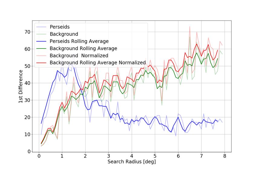
meteoroid detection is directionally dependent.
Keywords: Meteors, Interstellar meteoroids, Radar observations,
Interplanetary dust

1. Introduction

   Interstellar meteoroids offer a source of direct sampling of material that
originated from beyond our solar system. Presolar grains embedded within me-
teorites already provide samples of small solids formed in other star systems
(Zinner, 2014), but the particular system where such grains are produced is
unknown. Observations having trajectory information of large (>10 µm) in-
terstellar meteoroids may retain information on their source region as well as
providing clues as to the environment through which they traversed before be-
ing detected, as such large particles are not coupled to the local gas flow. Even
larger interstellar particles (ISPs) on the order >100 µm in radius (Murray et al.,
2004) may travel through the interstellar medium (ISM) for great distances with
little perturbation by Lorentz forces. Integrating the motion of these meteoroids
may allow for their original sources to be determined. Unique identification of
the stellar system from which a particular interstellar meteoroid originates can
help constrain the planet formation process, provide limits of the spatial density
of larger grains in the interstellar medium, and probe debris disks.
   Small interstellar particles have been directly detected in-situ in the solar
system by various spacecraft impact ionization sensors, including the Ulysses
(Grün et al., 1993), Galileo (Baguhl et al., 1995) and Cassini spacecraft (Alto-
belli, 2003), though the particle masses derived from impact sensors are very
uncertain. The impact-detected particles were on the order of 1 µm in radius
(10−14 kg) and smaller, assuming an average density of 3000 kg/m3 . Plasma
producing EM emission from impacts of micron-sized and smaller interstellar
particles have been detected by antennas on the STEREO (Zaslavsky et al.,
2012) and WIND (Wood et al., 2015) spacecraft. These measurements showed
that sub-micron interstellar dust shows a strong flux variation with time and

                                        2
orbital location. Such small particles are coupled to the local gas flow in the so-
lar neighborhood, which has an upstream flow direction in galactic coordinates
oflgal = 3°, bgal = 16° (Frisch et al., 1999) with a speed of 25 km/s. A good
review summarizing our understanding of the small interstellar dust detected in
the solar system is given by Sterken et al. (2019).
   The radar detection of interstellar meteoroids was reported by Baggaley
(2000) using the Advanced Meteor Orbit Radar (AMOR) in New Zealand and
by Meisel et al. (2002a) using the Arecibo radio telescope in Puerto Rico. Masses
and sizes of these detections were 9 × 10⁻⁹ kg (89 µm) and 7 × 10⁻¹¹ kg (18 µm),
respectively, again assuming a meteoroid density of 3000 kg/m3 . However, the
veracity of these detections as real interstellar meteoroids has been questioned
by other authors (eg. (Hajduk, 2001; Murray et al., 2004; Musci et al., 2012)).
   Hajduková et al. (2013) examined a catalogue comprised of 64650 mete-
ors observed by a multi-station video meteor network in Japan between 2007
and 2008 (SonotaCo, 2009). Of these detections, 7489 appeared to have hyper-
bolic orbits. After filtering for meteors with low error in measured velocity and
rejecting meteors associated with showers, 238 retained hyperbolic orbits and
showed no prior significant gravitational perturbations from close encounters
with planets within our solar system. Their main conclusion, that most appar-
ently hyperbolic optically measured meteoroid orbits are due to measurement
error, is similar to the main conclusion from other similar studies [eg. Musci
et al. (2012); Hajduková (2012)].
   Murray et al. (2004) provided estimates for the flux of interstellar particles
and examined potential ISP-producing sources. They suggested the most prolific
source would be dust grains produced as condensates in the atmospheres of
asymptotic giant branch stars, which are blown into the ISM by stellar winds.
Other sources they considered included dust grains from young main-sequence
stars ejected by dynamical interactions with planets, and dust ejected due to
radiation pressure from a host star. Additionally, they identified dust grains
emitted from high-speed narrow jets formed during the accretion phase of young
stellar objects to be a possible source of interstellar meteoroids. Weryk & Brown

                                        3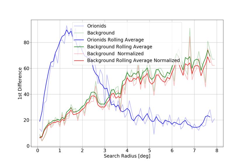
(2005) analyzed data collected by the Canadian Meteor Orbit Radar (CMOR)
between May 2002 and September 2004, where more than 1.5 million meteor
orbits were computed. From this study, 40 meteoroids were found to have
heliocentric speeds 2σ above the hyperbolic limit, and 12 of these meteoroids
had heliocentric speeds 3σ above the hyperbolic limit.
   The present study may be considered an extension to the work of Weryk
& Brown (2005). Here we expand on that study, in particular, by examining
CMOR echoes collected on six receiver stations (five remote, as compared to only
two available remote stations for the previous study). These additional stations
significantly increase the confidence in time of flight velocity solutions, compared
to the minimum three required for a unique time of flight solution as was the
case for the earlier Weryk & Brown (2005) study. We also develop an improved
velocity correction for atmospheric deceleration for CMOR echoes based on
examination of shower-associated meteors. This improves our confidence in
derived out-of-atmosphere velocities and therefore calculated heliocentric orbits.
   The discovery of 1I/ ‘Oumuamua, in 2017 (Meech et al., 2017) was the first
definitive observation of a large interstellar object transiting through our solar
system. A two day observation arc established that the orbit of ‘Oumuamua
was hyperbolic. Over 200 subsequent observations over 34 days provided a
more accurate assessment of its orbit and detailed lightcurve measurements
provide information on its size, morphology (Trilling et al., 2018), and clues
to its composition (Jewitt et al., 2017). The present study uses the orbital
elements of ‘Oumuamua, as a test case to model whether CMOR could detect a
hypothetical hyperbolic meteoroid stream of ‘Oumuamua-associated meteoroids.

2. Instrumentation and Initial Data Processing

   The Canadian Meteor Orbit Radar (CMOR) is a multi-frequency HF/VHF
radar array located in Tavistock, Ontario, Canada (43.26°N, 80.77°W). It con-
sists of a main site three-element Yagi-Uda vertically directed antenna as a
transmitter, five co-located receiving antennas, and five additional remote sta-

                                         4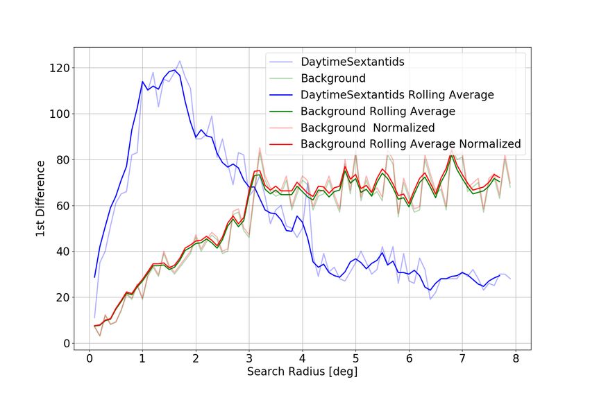
tion receivers. All receiver antennas are two-element vertically directed Yagi-
Uda antennas. The five receiving antennas at the main site are arranged as an
interferometer, allowing for positional measurements of meteor echoes (Jones
et al., 2005) with accuracy of order 1◦ . CMOR operates at 17.45, 29.85 and
38.15 MHz; however for this study only data collected from the 29.85 MHz
radar was used, as that frequency alone has orbital capability. More details of
the operation and hardware of the CMOR system can be found in Webster et al.
(2004); Jones et al. (2005); Brown et al. (2008).
   CMOR transmits Gaussianly-tapered radar pulses which are reflected off
the electrons left behind by the meteoroid ablating in the atmosphere. Only
the portion of these meteor trails which are oriented orthogonal to the receiver
station (ie: their specular points) are detectable at a particular receiver through
transverse scattering (see eg. Ceplecha et al. (1998)). With three or more re-
ceiver stations and interferometric (echo direction location in the sky) capability,
complete trajectory and time-of-flight velocity measurements can be obtained
(Jones et al., 2005). Confidence in time-of-flight velocity measurements increases
with the number of remote receiver stations, as the velocity solution becomes
over constrained beyond the minimum of three stations required for a velocity
solution.
   For CMOR, meteor echoes detected at multiple receiver stations are auto-
matically correlated and trajectories automatically computed (Weryk & Brown,
2012a). In addition, meteor echoes are automatically filtered to remove dubi-
ous or poor-quality echoes. The Fresnel phase-time method (hereafter referred
to as “pre-t0”) is also employed as a validation check on meteor speed. This
method is described in detail in Ceplecha et al. (1998). Pre-t0 velocities are
automatically computed from echoes detected at the main receiver station (T0)
as described in Mazur et al. (2019).
   The 29.85 MHz system transmits at 15kW peak power using a pulse rep-
etition frequency of 532 Hz, and has an effective collecting area of between
approximately 100 and 400 km2 (Table 1), dependent on the radiant decli-
nation (Campbell-Brown & Jones, 2006). Using the equations from Verniani

                                         5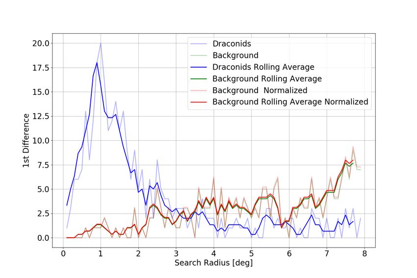
(1973) we estimate that the minimum detectable meteor magnitude for orbit
measurements under the requirement of detection at all six stations is +6 mag,
corresponding to a meteoroid diameter of approximately 400 µm at a velocity
of 45 km/s with an effective limiting mass of 1.8 × 10⁻⁷ kg. CMOR has been
in near continuous operation since 2002 with various upgrades to transmitter
power and the addition (and repositioning) of remote receiver stations. It has re-
mained in its present configuration since late 2011. Data collected for this study
spans January 2012 through June 2019 when all transmit and receive locations
and parameters were constant. In total, during this time period, 11073016 radar
meteor orbits were recorded.

  Transmitter Location                             43.26°N, 80.77°W
  Frequency                                        29.85 MHz
  Pulse Repetition Frequency                       532 pps
  Sample Rate                                      50 ksps
  Range Sampling                                   3 km
  Peak Transmit Power                              15 kW
  Minimum detectable echo Power                    10−13 W
  Collecting Area                                  100-400 km2
  Magnitude Limit                                  +8 (+6 for six station orbits)
  Height Range                                     70-120 km
  No. of Receiver Stations                         6
  Data Collection Dates                            January 2012 - June 2019
  Total orbits measured                            11073016
  Number of 6 Station orbits Recorded              395973

Table 1: Parameters of the 29.85 MHz CMOR orbital system and the experimental configu-
ration for this study.

                                          6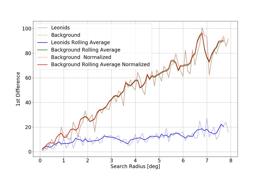
3. Searching for Interstellar Meteoroids in CMOR Data

3.1. Filtering

   CMOR multi-station echoes collected between January 2012 and June 2019
were examined to find evidence of interstellar meteoroids. This data set com-
prised over 11 million individual multi-station echoes for which time of flight
velocities could be determined. We restricted our search to those echoes recorded
on all six receiver stations - this yielded 395973 echoes. This was done as using
all receiver stations gives the most accurate velocities.
   Among this dataset, we further selected only events which appeared to have
hyperbolic heliocentric trajectories as computed from the raw (uncorrected)
measured time of flight velocities (Vm ). This produced 7282 candidate events
for initial examination. Finally, we limited our search to events with estimated
velocity errors of
etry (meaning the directional solutions for all pairwise antenna combinations
converge to one and not multiple solutions (Jones et al., 1998)) and “smooth”
amplitude profiles such that the profiles are consistent with the expected signal
affected by ambipolar diffusion, which should produce a smooth exponential
amplitude decay after the peak (Ceplecha et al., 1998) . While echoes are au-
tomatically correlated across receiver sites and trajectories computed without
manual intervention for these selected echoes, a detailed manual analysis is es-
sential to remove bad measurements.
   We performed detailed inspection of the amplitude vs. time profile of echoes
at all six receiver stations, compared automatic and manual selection of time
picks for time-of-flight velocities, and examined interferometry solutions. We
also compared rise time speed, Fresnel amplitude oscillation speed and Fresnel
phase slope (pre-t0) speeds to the time of flight velocity for consistency. In
addition to these quality controls, to check the overall robustness of each tra-
jectory solution we removed individual receiver station time picks to verify that
the computed velocity was minimally affected by removal of any one station,
typically showing solution differences in speed of less than 5% .

3.2. Results: Possible Interstellar Candidates based on Raw Measured Velocity

   After applying all filters and completing manual examination, a total of five
apparently hyperbolic events were identified. These events had time of flight
velocities consistent with calculated pre-t0 velocities, calculated rise time ve-
locities and, when visible, calculated Fresnel amplitude-time velocities (method
described in Ceplecha et al. (1998)). The observed in-atmosphere radiant and
speeds (without deceleration correction) in all cases produced hyperbolic orbits.
Potentially erroneous interstation echo matches were checked by removing in-
dividual receiver stations from the calculated solution and verifying that the
computed orbits remained consistently hyperbolic.
   These five events are summarized in Table 2 and the amplitude profile for
each station given in Figure 1. We emphasize that these events are hyperbolic
as measured with time of flight in-atmosphere measured speeds. These time of

                                       8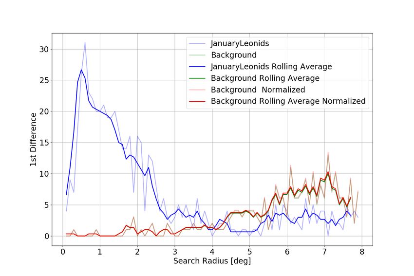
flight speeds represent the average over the height range of specular points across
       all six stations. As these speeds are lower than top of the atmosphere speed
       due to atmospheric deceleration in reality these should be more hyperbolic than
       observed, as described later. We examine the uncertainties in these quantities
       in the next sections.

   Event              η          ρ           Vc         Vm          Vf         Vt0           H0,1,2,3,4,5
                   [deg]       [deg]      [km/s] [km/s] [km/s] [km/s]                             [km]
2014-268-1026      73.37      174.34       41.16      40.00       38.53        37.2      90.5, 89.0, 91.1,
                                                                                         86.8, 92.1, 89.7
2015-008-1D0C      40.21       85.30       24.31      23.90       N/A         22.96      89.6, 88.6, 91.2,
                                                                                         94.6, 92.1, 90.9
2014-004-0805      79.50       -90.45      50.15      49.10       N/A        39.85*      95.6, 96.6, 97.3,
                                                                                         91.2, 92.8, 94.6
2017-283-2484      46.31      -144.81      43.24      41.20       N/A         42.24      101.4, 101.8, 100.9,
                                                                                         103.9, 101.2, 102.0
2014-299-0152      36.55      -161.39      43.18      42.20       N/A        35.57**     91.9, 93.7, 90.6,
                                                                                         98.2, 90.7, 93.6

       Table 2: Trajectories of candidate interstellar meteors as measured by CMOR. The event
       name tag is year-Solar-longitude followed by a unique internal file name for a particular echo.
       Here η is the local zenith angular distance of the apparent radiant, ρ is the local azimuth of
       the apparent radiant, measured counter-clockwise as seen from above from due East, Vc is
       the deceleration corrected velocity at the top of the atmosphere (used to compute the orbit -
       see 4), Vm is the measured time of flight speed in the atmosphere, Vf is the fresnel amplitude
       velocity (if available), Vt0 is the pre-t0 velocity and H0,1,2,3,4,5 is the height of the specular
       point from each receiver station, where the main transmit/receiver station is station 0. *Note:
       Vt0 automatically calculated from the method described in Mazur et al. (2019) for event 2014-
       004-0805 was 39.85 km/s far below Vm of 49.10 km/s. This appears to be an edge case scenario
       where the automatic pre-t0 velocity calculation fails. Manual inspection of the pre-t0 velocity
       shows that it is 49.87 km/s, consistent with Vm .** Similarly, manual inspection of the pre-t0
       for this echo shows a speed closer to 39 km/s.

                                                       9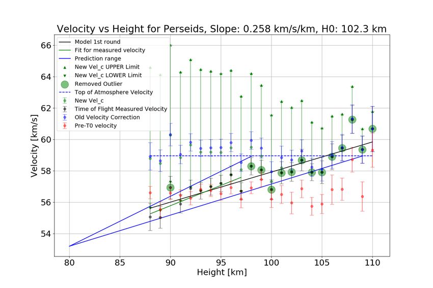
Event 20140119-091224 Event 20140325-062518
5000 Vm = 42.2 km/s station 0 Vm = 49.1 km/s station 0
Height = 91.9 km 5000 Height = 95.6 km
2500 = 36.6 deg = 79.5 deg
= 161.4 deg = 90.4 deg
0 0
station 1 20000 station 1
20000
10000 10000
0 0
station 2 station 2
10000
Amplitude [DU]
Amplitude [DU]
5000
5000
0 0
4000 station 3 station 3
5000
2000
0 0
4000 station 4 station 4
5000
2000
0 0
station 5 5000
station 5
4000
2000 2500
0 0
200 300 400 500 600 700 200 300 400 500 600 700
Pulse Pulse
Event 20141220-113805 Event 20150330-033813
5000 Vm = 40.0 km/s station 0 Vm = 23.9 km/s station 0
Height = 90.5 km 5000 Height = 89.6 km
2500 = 73.4 deg = 40.2 deg
= 174.3 deg = 85.3 deg
0 0
station 1 station 1
20000 10000
0 0
20000 station 2 station 2
10000
Amplitude [DU]
10000
Amplitude [DU]
0 0
4000 station 3 station 3
4000
2000 2000
0 0
2000
station 4 station 4
5000
1000 2500
0 0
5000 station 5 station 5
5000
2500
0 0
200 300 400 500 600 700 200 300 400 500 600 700
Pulse Pulse
Event 20170104-083955
5000 Vm = 41.2 km/s station 0
Height = 101.4 km
2500 = 46.3 deg
= 144.8 deg
0
20000 station 1
10000
200000 station 2
Amplitude [DU]
10000 Figure 1: Amplitude versus pulses (time) plots at each receiver
0 station of the candidate interstellar events. Green lines represent
station 3
4000
inflection points, red lines represent peak points.
2000
0
station 4
4000
2000
40000 station 5
2000
0
200 300 400 500 600 700
Pulse
103.3. Monte Carlo Simulation
To establish the significance of the hyperbolic excess speeds as measured,
we need to estimate uncertainties for each echo. To do this, we performed
Monte Carlo simulations of each meteor echo by randomly varying parame-
ters drawn from empirically derived error distributions estimated directly from
CMOR data. Many of these empirical estimates for error were based on six-
station CMOR detected shower echoes (see Section 4). This simulation uses the
observed geometry, range, interferometry, and speed of each echo and generates
a synthetic echo based on the ideal transverse scattering amplitude vs. time
profile produced by solving the Fresnel integrals (see Weryk & Brown (2012b)).
The CMOR time inflection pick algorithm and interferometry algorithm is
then applied to estimate the model speed. Uncertainties in range were simulated
by varying the observed range ± 1.5 km in a uniform distribution, representing
a precision of one full range gate (3 km) (Brown et al., 2008). The mean signal-
to-noise ratio (SNR) at receiver station 0 (main site) for all six station echoes
was found to be 20.3 (Figure 2). Mean SNRs for stations 1,2,3,4 and 5 were
11.8, 12.6, 14.5, 16.4 and 17.9, respectively. Standard deviation of errors in the
echo direction (interferometry) were found to be on average 0.159 degrees (rep-
resenting a positional uncertainty of 300m at 100 km range) from examination
of 160213 meteors (Figure 3) which were selected based on the methodology
described in Section 4. For the simulations, a more conservative value for inter-
ferometry uncertainty of 1 degree was used, consistent with differences between
optical and interferometric specular points measures for CMOR reported in past
studies (Weryk & Brown, 2012a).
Finally, uncertainty in time picks for inflection points of echoes is varied
over a random (assumed to be) gaussian distribution for time picks which were
found to have a standard deviation of approximately 1 pulse or 1/532 second
(Figure 4) based on examination of all six station meteors (Table 3). Here the
time pick uncertainty is estimated by noting the difference between the observed
time pick and the overall trajectory best-fit time pick per echo and per station
- it represents the observed empirical spread in time picks across all six station
11trajectories.
Histogram (normalized) of SNR n=160213 at st0
0.10 Gaussian fit
= 20.283
median = 20.100
= 3.995
0.08
Normalized count
0.06
0.04
0.02
0.00
5 10 15 20 25 30
SNR
Figure 2: Signal-to-noise ratio at receiver station 0 (main site) for all six station meteor echoes
with orbital measurements. The plot is normalized to our bin sizes such that the total area
under the curve is unity.
Error Paramater Error Value Distribution
Range 1.5 km [±] random, uniform
Interferometry 1 degree [SD] random, gaussian
Time picks 1 pulse (1/532 seconds) [SD] random, gaussian
Table 3: Error parameters used as input to Monte Carlo simulations for interstellar candidate
meteors detected by CMOR.
This Monte Carlo procedure can be applied to either the directly measured
velocities Vm or to the deceleration corrected velocity Vc providing distribu-
tions of significance in the individual hyperbolic measurements. To estimate
12the deceleration correction which should be applied to the observed speed to
recover the initial pre-atmosphere speed, we would need to know in detail the
ablation behaviour of a particular echo, information which is not available. To
approximate this correction, we instead use shower meteor echoes identified in
the CMOR data set and bootstrap our observed speed to the “reference” shower
speed. This provides a correction as a function of speed and height. The result-
ing average correction is applicable to CMOR-sized meteoroids and cannot be
easily applied to other systems.
A similar approach using much less data and less secure meteor shower speeds
was attempted by Brown et al. (2005a). We also explored the deceleration
dependence on entry angle and found it to be much less significant than the
height and speed dependence and hence omit entry angle from the correction.
We develop this deceleration correction in the next section.
13Figure 3: Histogram showing the mean interferometry solution residuals (in degrees) for sta-
tion 0 from examination of 160213 meteors detected on all 6-stations. More details are given
in Section 4.
14Figure 4: Histograms of mean time pick differences
(in seconds) for stations 1-5 between observed and
computed solutions from examination of 160213 me-
teors meteors recorded on all 6-stations. This pro-
vides an empirical estimate of the time pick uncer-
tainty which is then used in the echo Monte Carlo
simulations. Note that the timing is relative to T0
(the main site) and that 1 pulse represents a timing
difference of 1.8×10⁻³ sec.
154. Deceleration Correction
A more accurate deceleration correction for meteor echoes detected by CMOR
allows for improved pre-atmosphere velocity determination leading to more ac-
curate orbit calculations. In particular, this correction provides our best statis-
tical estimate to the true top of atmosphere velocity, recognizing that all our
candidate events have measured in-atmosphere speeds which already produce
hyperbolic orbits.
Shower meteors, being on common orbits (by definition) should have similar
entry velocities. There is, however, no accepted quantitative metric for shower
association, but we will attempt to define some criteria to use for our study in
Sections 4.1 and 4.2. However, there may be some spread in velocities based on
time of occurrence in the shower (ie. velocity changes with solar longitude) or
with meteoroid mass. Several surveys have previously estimated initial shower
velocities. In the past these have applied a deceleration model (Jacchia & Whip-
ple, 1961) to estimate the pre-atmosphere speed. Ideally, measuring shower me-
teoroid velocities at very high heights, before deceleration becomes significant, is
better. A dataset of shower meteors which uses the latter approach for the first
time was recently collected by the Middle Atmosphere Alomar Radar System
from head echo shower measurements (Schult et al., 2018), which are detected
at very high (typically above 100 km) height and have very precisely measured
doppler speeds. We adopt MAARSY shower speeds when available as the most
probable “reference” pre-atmosphere speed.
Since the total deceleration depends on the amount of atmosphere encoun-
tered for a fixed mass meteoroid (eg. Ceplecha et al. (1998)), in general, we
expect the measured speed of a particular shower echo to depend most signif-
icantly on height, though entry angle and physical structure may also play a
secondary role. However, the height at which initial deceleration occurs for simi-
lar masses will be velocity dependent as the starting height for ablation is speed
dependent (Koten et al., 2004; Hawkes & Jones, 1975) as is the intercepted
momentum per unit atmospheric mass.
16We examined the average measured time-of-flight velocity (Jones et al., 2005)
from CMOR shower echoes within specific height bins to find the average shower
velocity for typical CMOR echoes as a function of height. The basic approach
follows the procedure outlined in Brown et al. (2005b). However, this study uses
a much larger sample and more recently measured values for initial (“reference”)
shower velocities.
We used the literature value of reference speed to estimate the height at
which shower echoes show no noticeable deceleration relative to the top of at-
mosphere, which we term H0 . For CMOR, this varies from roughly 95 km
at slow speeds to 105 km for higher speed meteoroids. The associated slopes
(change in speed per km below the H0 height) and H0 are determined for several
showers spanning a spread of velocities. We found that linear fits reproduced
the observed speed vs. height behaviour for most showers. Thus, linear fits for
slope and H0 were determined for each shower. These fits as a function of speed
are then combined into a single correction term as a function of specular height
and time-of-flight speed which can then be applied to any CMOR echo to give
a best-estimate for its pre-atmosphere speed.
The resulting fit confidence bounds in slope and H0 as a function of velocity
place limits on the total correction as well as a best estimate for the nominal
correction. Data collected from CMOR between January 2012 and December
2018 was used to estimate this velocity correction.
We use as ground-truth top of atmosphere reference velocities for known
showers reported by MAARSY (Schult et al., 2018) where possible and other-
wise literature sources (Table 4) summarized on the IAU Meteor Data Center
established shower list 2 . The literature sources vary in their estimates of veloc-
ity. Therefore, velocities which are closest to the observed CMOR values where
noticeable deceleration begins are chosen. For meteors from a particular shower,
we take CMOR measured velocities that fall between ± 20% of the expected
top of atmosphere velocity (based on the literature values) for a meteor shower
2 https://www.ta3.sk/IAUC22DB/MDC2007/
17for expected velocities of 40 km/s. This
includes extremely decelerated meteors (≈5 km/s) at heights as low as ≈80
km. As lower velocities can be measured with greater precision with CMOR
(due to the larger time offsets between stations), we use a smaller spread in
velocities (20%) for these velocities compared to 30% used for faster velocities
which are measured less accurately. The expected Vinf (expected velocity at top
of atmosphere) were taken from literature values (Table 4) using the expected
geocentric velocity (Vg ) of a shower and adding the acceleration due to gravity
of the Earth taken from infinity (Equation 1). Vesc is taken to be the escape
velocity of the Earth at 100 km above the surface, 11.1 km/s.
q
Vinf = Vg 2 + Vesc 2 (1)
Only meteor echoes with individually estimated velocity (Vm ) errors ofShower IAU Vg Vinf Source
code [km/s] [km/s]
Daytime Arietids ARI 38.6 40.2 Schult et al. (2018)
Daytime Sextantids DSX 31.2 33.1 Galligan & Baggaley (2002)
Draconids DRA 20.7 23.5 Jenniskens et al. (2016)
Geminids GEM 33.1 34.9 Schult et al. (2018)
January Leonids JLE 51.4 52.6 Jenniskens et al. (2016)
Leonids LEO 69.3 70.2 Schult et al. (2018)
November Omega Orionids NOO 42.7 44.1 Schult et al. (2018)
Orionids ORI 66.3 67.2 Jenniskens et al. (2016)
Perseids PER 57.9 59.0 Molau (2007)
Quadrantids QUA 40.0 41.5 Schult et al. (2018)
Southern Delta Aquarids SDA 39.4 41.0 Molau (2007)
Xi Coronae Borealids XCB 44.9 46.3 Schult et al. (2018)
Table 4: Literature sources used for reference Vg and Vinf velocities for shower meteors.
19Shower λ−λ β Peak Peak Spread Radius
[deg] [deg] [λ ] [date] [days] [deg]
Daytime Arietids 331.0 8.0 77 8-Jun 5 4.4
Daytime Sextantids 329.6 -11.5 189 2-Oct 4 3.0
Draconids 51.7 77.6 195 8-Oct 1 3.8
Geminids 208.0 10.5 261 13-Dec 10 4.2
January Leonids 219.0 10.2 282 3-Jan 3 3.5
Leonids 272.0 10.0 237 20-Nov 5 5.0
November Omega Orionids 203.5 -7.8 247 29-Nov 3 2.8
Orionids 247.0 -7.8 208 22-Oct 5 3.5
Perseids 282.0 38.5 140 13-Aug 5 3.0
Quadrantids 277.0 63.2 283 4-Jan 2 5.5
Southern Delta Aquarids 210.2 -7.3 124 27-Jul 3 3.5
Xi Coronae Borealids 301.5 51.5 296 16-Jan 2 5.0
Table 5: Shower parameters used to associate individual echoes with a particular shower. This
is based on the 3D-wavelet analysis methodology applied to CMOR velocities (Brown et al.,
2010) using all radiants recorded between 2002-2016. Here the spread refers to the number of
days around the maximum the shower was detectable and/or showed radiant motion in sun-
centred coordinates was less than one degree. Radius refers to the size of the radiant area about
the point of maximum where radiant density is above the background. The ecliptic longitude
and latitude of the radiant is given by λ and β respectively, while the solar longitude is λ .
4.1. Radiant Selection
The radiant of a particular shower in sun-centred ecliptic coordinates were
taken from the λ − λ0 , β of the shower during the peak solar longitude bin,
as measured by CMOR using the 3D wavelet procedure described in Brown
et al. (2010) as shown in Table 5. Here all CMOR radiants from 2002 - 2016
were combined to better estimate the shower radiant and its drift. λ − λ0 and
β were used to select shower echoes as radiant drift is minimal in sun-centred
coordinates for any given shower.
The solar longitude (λ ) of peak activity is defined as the solar longitude
20(in the J2000.0 equinox) with highest wavelet coefficient excursion over the
annual background at the same sun-centred ecliptic coordinates averaged over
the entire year (excluding the shower activity interval) as described in Brown
et al. (2010). The range of solar longitudes used to identify individual CMOR
shower echoes with a specific shower is based on the time of peak activity and
the wavelet determined observed radiant (λ − λ0 and β) at the peak. From this
starting point, we included only the days before and after the peak where the
sun-centred radiant as measured by the wavelet procedure described in Brown
et al. (2010) remains within 1 degree of λ − λ0 and β values at the peak, a value
much smaller than our radiant selection radius.
4.2. Radiant Selection Radius
The radiant selection radius is the maximum angular separation in the sky
we adopted between the CMOR wavelet measured radiant at peak activity and
the radiant of an individual CMOR echo used to associate a meteor radiant
as being part of the shower. To establish this radius for each shower we first
estimated the background density of sporadic radiants at the same sun-centred
ecliptic coordinates. Starting from the nominal sun-centred shower radiant we
expect the radiant density to fall as the radius is increased; once the density
reaches the background, we declare this the effective shower selection radius.
This follows a similar procedure described in Ye et al. (2013).
This involves first using an initial radius of 8 degrees from the shower radiant
and counting all meteor echo radiants which fit the above criteria. A background
count of sporadic meteors with the same velocity restrictions is also taken at the
same sun-centred location starting with an 8 degree radiant radius but separated
in time by ± (2 × day spread + 5 degrees of solar longitude) beyond the shower
activity interval (defined from the wavelet duration of the shower) plus the day
spread. This is done in order to ensure that equal time windows (and hence
collecting area - time products) are used for both the intervals where shower
meteors are counted and background meteors counted. If there is a difference
between the total number of days used for shower meteor counts and the total
21number of days used in background meteor counts (i.e. in some cases there
were no days with recorded data due to radar downtime), then the count of
background meteors is normalized to the number of collection days used to
identify the shower meteor echoes.
As an example, for the 2002-2016 Geminid shower (Figure 5), the total
shower duration is 2 × 10 days, and 20 days of background meteors are taken
outside this interval starting 25 days before and 25 days after the shower activity
period. But there are 3 days of radar dropouts, so the background meteor counts
would be multiplied by 20/17 to correct for this.
40000 Wavelet 2.0
Peak Sep.
Radiant Separation from Peak [deg]
35000
30000 1.5
Wavelet Coefficient
25000
20000 1.0
15000
10000 0.5
5000
0 0.0
250 255 260 265 270
Solar Longitude [deg]
Figure 5: Geminid meteor shower activity from stacked wavelet radiant measurements col-
lected between 2002 and 2016. The total day spread for an angular separation of wavelet-
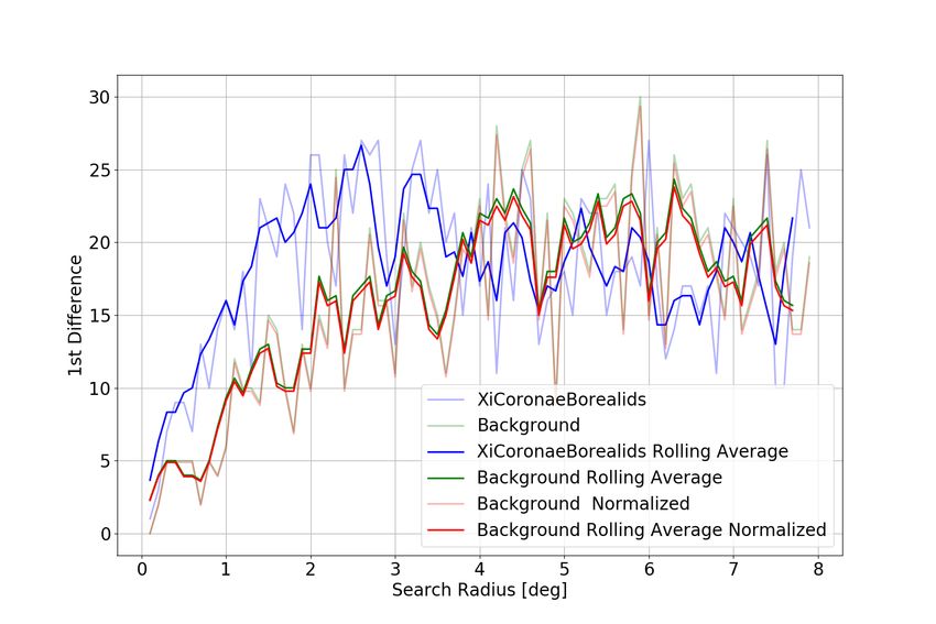
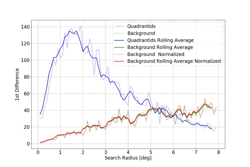
determined observed radiant (λ − λ0 and β) from peak activity ≈creased in 0.1 degree steps for both the shower meteor radiant search area and
the background sporadic meteor radiant search area, within their respective
time windows. A first difference in count numbers between each successive de-
crease in search radius is calculated and a running average of 0.3 degrees of
the count is then computed (Figure 6). The radius at which the rolling aver-
age of the first difference in the count for the shower radiants crosses the first
difference in the count of the background sporadic meteor radiants is taken to
be the radius over which meteor radiants can be reliably associated with the
shower without significant background contamination. This becomes the search
radius used for that particular shower (Figure 7) in our deceleration analysis.
Only meteor echoes with individual radiant uncertainties, as determined from
the Monte Carlo procedure described in Weryk & Brown (2012b), of less than
1 degree are included.
Figure 6: A 1st-difference of meteor radiant counts as a function of search radius about the
Geminid radiant during its activity period and the same for sporadic meteor radiants at the
same sun-centred location 25 days after the peak.
23DaytimeArietids shower (Sun Centered Ecliptic Radiants) 160
Shower Search Area
Radiant Extents
15.0 140
12.5 120
100
10.0
Meteor Count
[deg]
80
7.5
60
5.0
40
2.5
20
0.0
0
322.5 325.0 327.5 330.0 332.5 335.0 337.5 340.0
- 0 [deg]
Figure 7: Density plot of radiants for the Daytime Arietids with the shower search area
(white dashed circle) overlaid for comparison. Green dots and line represent the extent of
the radiant drift between the start and end of the search period based on the stacked wavelet
radiant location as described in the text.
Large uncertainties in radiant solutions are often caused by meteor echoes
which have specular points from multiple stations very near each other along the
trail. Such echoes have very small difference in timing across different receiver
stations. This decreases the accuracy of the time of flight velocity measurement.
When the echo amplitudes as a function of time are plotted per station, the
inflection points for these echoes appear to occur in or near a straight vertical
line as shown in Figure 8. We wish to remove these meteors from further analysis
as they have large uncertainties. From empirical tests where we compared the
Monte Carlo error in Vm with the time lags, we arrived at a criteria for rejecting
24meteor echoes not having sufficient time delays for good velocity solutions as
being when the average time offset between echoes measured relative to the
main (T0) receiver/transmitter station and other receiver stations as described
in Equation 2.
Event 20150114-083056 Event 20131201-001233
station 0 station 0
10000 VHeight
m = 71.1 km/s
= 97.0 km
20000 Vm = 41.5 km/s
Height = 92.9 km
= 39.7 deg 10000 = 74.4 deg
= 55.5 deg = 24.7 deg
0 0
20000 station 1 station 1
5000
10000
0 0
station 2 20000
station 2
20000
Amplitude [DU]
Amplitude [DU]
10000 10000
100000 0
station 3 station 3
5000 10000
0 0
station 4 station 4
5000 10000
5000
0 0
station 5 20000 station 5
5000 10000
0 0
200 300 400 500 600 700 200 300 400 500 600 700
Pulse Pulse
Figure 8: An echo detected at 6-stations showing amplitude versus time for each site. Event
20150114-083056 shows bad timing spread where inflection points appear in near vertical line
and all coincide in time. The error in TOF speed for this event is 135.93 km/s. Event
20131201-001233 shows good timing spread where inflection points are spread out. The error
in TOF speed for this event is 0.12 km/s. Green lines represent inflection points, red lines
represent peak points. The time of flight speed and specular height (as measured by inter-
ferometry from station 0) are given in the upper left of each sub-caption. The local radiant
zenith angle (η) and azimuth (ρ) are also shown.
Vg
Offset = × 0.1s (2)
VGeminids
The Geminid meteor shower was used for calibration of this selection filter.
For the Geminids, we removed meteor echoes with average time offsets below
0.1 seconds (roughly 5 pulses) for the Geminids. This minimum offset value was
25then scaled proportional to the shower velocity relative to the Geminid velocity.
Two showers were not filtered for time offsets: the Draconids, where including
this offset filter left too few echoes for analysis (less than five useable height
bins), and the Perseids, whose average path lengths (≈7 km) are significantly
shorter than the path lengths of other showers (≈10 km) and whose speed is
very high (60 km/s) resulting in necessarily small offsets.
4.3. Estimation of Deceleration Slope and H0
After filtering using the foregoing criteria, average measured time of flight
velocities, pre-t0 velocities, the cosine of local zenith angular distance of appar-
ent radiant, and echo ranges (among other parameters) were computed in 1 km
height bins between 80 km up to 120 km for each shower, and the standard error
of these averages also calculated. Bins which contain less than 10 meteors are
ignored. Plots were created of average measured velocity, pre-t0 velocity, cosine
of the local zenith angular distancge of apparent radiant (η), path length (cal-
culated as the time of flight × difference between minimum and maximum time
offsets of receiver stations) as a function of height. These plots are shown in the
appendix. Additionally, the location of the main site specular point (which de-
termines the height) as a fraction of the total trail length was computed. These
plots were generated for each shower and were manually inspected to ensure
that they followed expected trends, which include:
• Cosine of η (radiant zenith distance) should remain approximately con-
stant or vary monotonically with respect to height (Figure 9), with lower
height bins on average accessible for more steep (lower η) entries. Note
that the entry angle is also correlated with the speed as a function of
height and is related to the local radiant height through the specular re-
flection condition; ie. low entry angle trajectories are always associated
with high local echo elevations.
• The fraction of the echo path length observed before the station 0 specular
point should decrease with height (Figure 10). That is we expect the main
26site specular point to lie near the end of the trail as height decreases.
• The measured time of flight-based speed and pre-t0 speed should increase
with height and asymptotically approach Vinf quite sharply. We reject as
outliers time of flight velocity points above the crossing of Vinf / start of
plateau (Figure 11). The measured time of flight and pre-t0 velocities per
bin are expected to differ because the former is a measure of the average
speed over a larger segment of the trail, but the slope/trends should be
comparable.
Entry Angle vs ht for DaytimeArietids shower
0.7
0.6
0.5
Cos eta
0.4
0.3
82.5 85.0 87.5 90.0 92.5 95.0 97.5 100.0 102.5
ht [km]
Figure 9: Mean cosine of local zenith distance of the apparent radiant (η) versus height for the
Daytime Arietids. The uncertainty bounds per point represent the standard error of the mean
per bin. Here shallower entry angles are seen at preferentially higher heights, as expected.
27Avg Fraction before T0 vs height of DaytimeArietids
0.6
0.5
Fraction before T0 [frac]
0.4
0.3
0.2
82.5 85.0 87.5 90.0 92.5 95.0 97.5 100.0 102.5
Height [km]
Figure 10: The height here is the specular echo height as measured from station 0. For
all echoes in each height bin we calculate the mean fraction of the total observed meteor
trail length which occurs before the specular point, T0 as well as the standard deviation
(uncertainty bounds per bin). In this example we are using only echoes associated with the
Daytime Arietid meteor shower. The trend here is as expected, namely that the lower the
specular height as seen from the main station, the larger is the fraction of the trail which
occurs above this specular point - ie. the specular point is occurring near the end of the
measured trail at lower heights.
28Velocity vs Height for DaytimeArietids
42 Removed Outlier
Top of Atmosphere Velocity
41 Measured Velocity
PTN
40
velocity [km/s]
39
38
37
36
35
82.5 85.0 87.5 90.0 92.5 95.0 97.5 100.0 102.5
height [km]
Figure 11: The average and standard error of the mean of the measured time of flight and
pre-t0 (PTN) velocities per 1 km height bin for the Daytime Arietids. A general plateau in
the speed vs. height is evident above 96 km, particularly in the pre-t0 speeds which are a
better point estimate of speed.
Height bins which fall substantially outside of these expected trends from
visual inspection are added to an outlier list for each shower and are not included
in the final analysis.
Once outliers have been removed, a second linear fit to the measured velocity
(Vm ) versus height (H) is generated (Equation 3), weighted to the reciprocal of
the standard error of each average measured velocity. The slope coefficient (S
in km/s/km) of this fit and its intersection height (H0 in km) with the literature
Vinf are found for each shower (Equation 4) as:
Vm = Scoeff H + Sconst (3)
H0 = (Vinf − Sconst )/Scoeff (4)
294.4. Combining All Showers
The individual velocity vs. height slopes obtained for each shower as a func-
tion of Vinf are used to construct an overall linear fit. The deceleration slope
across all showers is generated from a linear fit weighted by the standard error of
each shower slope. If all meteoroids from different streams had similar physical
properties/masses and were observed under similar geometries we would expect
this slope to have a single value. This simply reflects the fact that the deceler-
ation is driven by the mass of atmosphere intercepted, which is independent of
speed.
The S versus Vinf , with a linear regression weighted by the count per shower
and 95% Confidence and Prediction Intervals shaded are shown in Figure 12.
While there is scatter, reflecting both physical differences between meteoroids,
the way they decelerate as well as variations in CMOR observing geometry
between showers, as shown in Table 6 the slope coefficient is within one standard
error of zero, much as expected from theory.
30Weighted fit
0.5 95% Confidence Interval
95% Prediction Interval
Shower, dot size = log count
0.4
Slope [km/s/km]
LEO
ORI
DRA GEM
0.3 ARIQUA
PER
XCB
DSX SDA
0.2
NOO JLE
0.1
20 30 40 50 60 70
Vinf [km/s]
Figure 12: Slope of the change in speed with height as a function of Vinf for all twelve
of the showers (identified by their three letter IAU designation) used for calibration of the
deceleration correction.
The H0 intercept as a function of Vinf across all showers is similarly obtained
by extracting the linear fit for each shower, which is weighted by the error in
H0 for each shower (Figure 13). This error is calculated by taking the extremes
of the H0 intercept for each shower from the velocity versus height slope ±
the standard error of the slope, beginning at the calculated slope’s intercept
at 80 km height. A height of 80 km was chosen as very few meteor echoes
were observed below this height and most meteors echoes observed between 80
km and the H0 intercept height would fall within the region contained between
the height slope ± standard error extremes. Equations 5 and 6 summarize the
resulting H0 limits.
31120 Weighted fit
95% Confidence Interval
115 95% Prediction Interval
Shower, dot size = log count
LEO
110
XCB
105 NOO
ORI
PER
H0 [km]
JLE
QUA
100 DRA ARI
DSXGEM SDA
95
90
85
20 30 40 50 60 70
Vinf [km/s]
Figure 13: The height at which negligible deceleration in shower meteors is measured by
CMOR, H0 , as a function of Vinf for all twelve measured showers.
Vinf − (80km × Scoeff − 80km × (Scoeff + Serror )) + Sconst
H0min = (5)
Scoeff + Serror
Vinf − (80km × Scoeff − 80km × (Scoeff − Serror )) + Sconst
H0max = (6)
Scoeff − Serror
As expected, the H0 value generally increases with speed, reflecting the
higher beginning heights of ablation for faster meteoroids (which therefore re-
ceive more energy per atmospheric molecule encountered), paralleling the in-
crease in beginning height with speed observed by optical cameras (eg. Ceplecha
(1968)). However, for heights ≈105 km, the echo height ceiling becomes signifi-
cant at CMOR’s 29.85 MHz frequency, so the trend at higher speeds also reflects
the lack of detectable echoes above this height as opposed to real differences in
beginning ablation heights.
32To independently assess how reasonable is our empirical estimate that H0
represents the height above which negligible deceleration occurs, we applied
the ablation modelling approach of Vida et al. (2018). We assumed that the
meteoroids were cometary and used a peak magnitude of +7 (appropriate to
the median size of CMOR detected echoes as described in Brown et al. (2008))
and examined the expected deceleration as a function of height. For the range
of values of H0 in Fig 13 we find that the Vida et al. (2018) formalism predicts
decelerations of order 0.5 km/s at the highest speeds (heights of 105 km) to
almost 1 km/s at speeds of 20 km/s for heights of 92 km.
It is notable that the Draconids in the lowest speed portion of the dis-
tribution is anomalous in that radar Draconids tend to begin deceleration at
higher heights than a simple extrapolation would predict from the other show-
ers. This reflects the well known fragility of the Draconids and their higher
starting heights (Koten et al., 2007) compared to other meteors of similar ini-
tial speed.
4.5. Final Velocity Correction
The H0 and S fit coefficients and constants (Table 6) are combined to obtain
a final measured velocity correction (Vc ) (Equation 7).
Vc = Vm − [(H − (H0fit fit fit fit
coeff Vm + H0const )) × (Scoeff Vm + Sconst )] (7)
This correction uses the observed echo height from the main site and the
time of flight speed to then estimate the equivalent average amount of velocity
correction needed to bring the meteoroid to the top of the atmosphere. This
general correction is applicable to all CMOR-detected meteor echoes, but should
not be applied to other systems.
Figure 14 shows the magnitude of the correction as a function of velocity for
various specular heights. Also shown are the corrections used by the Advanced
Meteor Orbit Radar (AMOR) (Baggaley, 1994) and the Harvard Radio Me-
teor Project (Verniani, 1973) (HRMP) together with the original deceleration
correction for CMOR given by Brown et al. (2005a).
33The largest difference between the old and new correction are for low veloci-
ties and low heights, where extreme differences of 2-3 km/s are found. However,
unlike the old correction which rolled over at high speeds for a given height (an
unphysical result), the new correction becomes linearly larger for both lower
heights and higher speeds. The new correction most closely resembles the mean
HRMP correction and is less than the AMOR correction. Since HRMP sampled
masses similar to CMOR while AMOR masses were much smaller this is both
physically consistent and more realistic than the earlier CMOR deceleration
correction. Note that for most heights and speeds the new and old corrections
differ by of order 1 km/s on average.
As an example application of the new correction, in Figure 15, we apply
the correction to the Daytime Sextantid shower. The resulting corrected speeds
better reproduce the expected top of atmosphere speed, showing a near constant
corrected speed as a function of echo height. In contrast, the earlier correction
from Brown et al. (2005a) (shown as blue symbols) tends to over correct the
speed, particularly at lower heights for this shower.
We obtain lower and upper limits encompassing the majority of the expected
distribution to the 1σ level for the velocity correction (Equations 10 and 13)
by applying the standard errors to the slope and H0 values (Table 6) for Slope
(Equations 9 and 12 and H0 (Equations 8 and 11 based on these fits. If the
lower limit falls below the measured velocity, then we use the measured velocity
as the lower limit.
H0lower = Vm (H0fit fit fit fit
coeff − σx̄ H0coeff ) + H0const − σx̄ H0const (8)
fit fit fit fit
Slower = Vm (Scoeff + σx̄ Scoeff ) + Sconst + σx̄ Sconst (9)
Vclower = Vm − [(H − H0lower ) × Slower )] (10)
H0upper = Vm (H0fit fit fit fit
coeff + σx̄ H0coeff ) + H0const + σx̄ H0const (11)
34Figure 14: New velocity correction for CMOR (red lines) as a function of height compared
to original correction (black lines) from Brown et al. (2005a). Also shown are the deceler-
ation correction used for AMOR (green line) (Baggaley, 1994) and for the Harvard Radio
Meteor Project (blue line) (Verniani, 1973). Note that both AMOR and HRMP used average
corrections with speed without an explicit height dependence.
35DaytimeSextantids
36
35
34
Velocity [km/s]
33
32
31
Fit for Vm
Vinf
30 New Vc
Vm
Old Vc
29 Vt0
84 86 88 90 92 94
Height [km]
Figure 15: Velocities versus height in 1 km height bins for the Daytime Sextandids.
fit fit fit fit
Supper = Vm (Scoeff + σx̄ Scoeff ) + Sconst + σx̄ Sconst (12)
Vcupper = Vm − [(H − H0upper ) × Supper )] (13)
36Parameter Value
H0fit
coeff 0.2726
fit
H0const 86.8152
fit
Scoeff 0.0012
fit
Sconst 0.2171
H0fit
coeff standard error 0.0950
H0fit
const standard error 3.8797
fit
Scoeff standard error 0.0013
fit
Sconst standard error 0.0720
Table 6: Parameter values used for velocity correction
Of the 12 showers used in calibrating the new velocity correction, ten showed
as good or was an improvement in the average velocity correction with height,
producing better agreement with literature values of top-of-atmosphere velocity
(Table 7) as compared to the earlier correction from Brown et al. (2005a).
37Shower no. of Vinf Mean Old Mean New
Meteors [km/s] Vc - Vinf Vc - Vinf
[km/s] [km/s]
Draconids 159 23.5 -0.9 -1.6
Daytime Sextantids 756 33.1 1.3 0.1
Geminids 7672 34.9 0.9 -0.4
Daytime Arietids 6023 40.2 0.6 -0.5
Southern Delta Aquariids 4051 40.9 2.1 0.9
Quadrantids 1629 41.5 0.0 -1.0
November Omega Orionids 685 44.1 0.6 -0.3
Xi Coronae Borealids 397 46.3 -1.0 -1.9
January Leonids 190 52.6 1.3 0.7
Perseids 427 59 0.3 0.0
Orionids 624 67.2 -0.3 -0.2
Leonids 112 70.2 -2.7 -2.5
Table 7: Comparison of old velocity correction to new velocity correction results (Vc ). Itali-
cized showers indicate smaller (absolute value) residuals between new Vc - Vinf versus old Vc
- Vinf , where Vinf is the literature value of top-of-atmosphere speed.
4.6. CMOR detected Interstellar Candidates with Deceleration Correction
We now apply our new deceleration correction to the measured time of flight-
derived velocities of all CMOR-detected candidate interstellar meteoroids fol-
lowing the procedure outlined in Section 4. This provides a more realistic esti-
mate of the top of atmosphere velocity, though we again emphasize that these
candidate events have measured nominal in atmosphere speeds which already
place them in hyperbolic orbits.
A Monte Carlo simulation (10000 runs) was performed for each of the five
interstellar meteoroid candidates as described in Section 3.3. Based on their ob-
served in-atmosphere speeds (Vm ), all five candidates showed eccentricities >2σ
above the hyperbolic limit with one event yielding >3σ for e >1 as summarized
38in Table 8. Upon applying the deceleration correction to estimate the “true”
speed, Vc , all five events showed >3σ for e >1.
Figure 16 shows the resulting Monte Carlo distributions of eccentricity for
four of these events based on both the measured time of flight speed (blue
histogram) and our best estimate of the deceleration corrected top of atmosphere
speed (red histogram). The most promising interstellar (IS) candidate which
showed >3.7σ for e >1 was event 2014-268-1026. This is shown in Figure 17.
Figure 16: Histogram of eccentricities based on 10000 Monte Carlo simulations of four inter-
stellar candidate CMOR echoes showing eccentricities derived from raw measured velocities
Vm (blue histogram) and corrected velocities Vc (red histogram). The eccentricity based on
the original measured speed, Vm is shown as a vertical dashed blue line while the nominal
eccentricity found after correcting for atmosphere deceleration is the vertical dashed red line.
39Event Mean e σ e >1 Mean e σ e>1
from Vm for Vm from Vc for Vc
2017-283-2438 1.12 3.4σ 1.12 3.5σ
2014-004-0805 1.12 2.9σ 1.17 3.4σ
2014-299-0152 1.08 2.3σ 1.11 3.2σ
2015-008-1D0C 1.09 2.0σ 1.16 3.3σ
2014-268-1026 1.08 2.9σ 1.12 3.7σ
Table 8: Eccentricities from Monte Carlo simulations for all five interstellar meteoroid candi-
dates calculated using raw measured velocities (Vm ) and atmospheric deceleration corrected
velocities (Vc ).
Figure 17: Histogram of eccentricities from 10000-run Monte Carlo simulations of the best
CMOR IS candidate event based on raw measured velocity Vm and corrected velocity Vc .
We summarize our best estimate for the orbital and radiant parameters for
each of our five candidate IS events in Table 9.
404.7. Estimated Interstellar Meteoroid Flux
To estimate the equivalent IS flux from our five possible CMOR echo detec-
tions, we need to determine the limiting mass and integrated collecting area-time
product of our survey.
The weakest echoes CMOR is sensitive to approaches +8.5 radio magnitude
(Brown et al., 2008) (equivalent to an estimated limiting electron line density of
≈ 2×10¹² e− /m). By limiting our survey to echoes which appear only on all six
receiver stations, we expect the limiting line density to be larger than this value.
Figure 18 shows the distribution of electron line densities for all six station
events in our data set showing that the effective completeness limit is near
2×10¹³ e− /m or close to radio magnitude of +6. Using the mass-magnitude-
velocity relation from Verniani (1973), this corresponds to meteoroid masses
on the order of 10−7 kg for events with in-atmosphere velocities of 45 km/s.
These are equivalent to diameters ranging from 400 µm for meteoroids with
bulk densities similar to asteroidal and chondritic meteoroids (4200 kg/m3 ), to
800 µm for meteoroids with similar bulk densities to meteoroids found in Halley
type orbits (360 kg/m3 ) (Kikwaya et al., 2011).
41You can also read