DNS-based characterization of pseudo-random roughness in minimal channels
←
→
Page content transcription
If your browser does not render page correctly, please read the page content below
This draft was prepared using the LaTeX style file belonging to the Journal of Fluid Mechanics     1

                                                                     DNS-based characterization of
arXiv:2106.08160v2 [physics.flu-dyn] 17 Jun 2021

                                                                  pseudo-random roughness in minimal
                                                                               channels
                                                             Jiasheng Yang1 , Alexander Stroh1 , Daniel Chung2 and Pourya
                                                                                      Forooghi3 †
                                                            1
                                                                Institute of Fluid Mechanics, Karlsruhe Institute of Technology, Karlsruhe, Germany
                                                       2
                                                           Department of Mechanical Engineering, University of Melbourne, Victoria 3010, Australia
                                                   3
                                                       Department of Mechanical and Production Engineering, Aarhus University, Aarhus, Denmark

                                                                                      (Received xx; revised xx; accepted xx)

                                                   Direct numerical simulation (DNS) is used to study turbulent flow over irregular rough
                                                   surfaces in the periodic minimal channel configuration. The generation of irregular
                                                   rough surface is based on a random algorithm, in which the power spectrum (PS)
                                                   of the roughness height function along with its probability density function (PDF)
                                                   can be directly prescribed. The hydrodynamic properties of the roughness, particularly
                                                   the roughness function (∆U + ) and zero-plane displacement (d), are investigated and
                                                   compared to those obtained from full-size DNS for 12 roughness topographies with
                                                   systematically varied PDF and PS at four roughness height (k + = 25 – 100). The
                                                   comparison confirms the viability of the minimal channel approach for characterization of
                                                   irregular rough surfaces providing excellent agreement (within 5%) in roughness function
                                                   and zero-plane displacement across various types of roughness and different regimes.
                                                   Results also indicates that different random realizations of roughness, with a fixed PS and
                                                   PDF, translate to similar values of roughness function with a small scatter. In addition to
                                                   the global flow properties, the distribution of time-averaged surface force exerted by the
                                                   roughness onto the fluid is examined and compared to the roughness height distribution
                                                   for different cases. It is shown that the surface force distribution has an anisotropic
                                                   structure with spanwise-elongated coherent regions. The anisotropy translates into a
                                                   very small streamwise integral length scale, which weakly depends on the considered
                                                   roughness topography, while the larger spanwise integral length scale shows a stronger
                                                   dependence on roughness characteristics. It is also shown that the sheltering model
                                                   proposed by Yang et al. (2016) describes well the spatial distribution of the streamwise
                                                   surface force. We also studied the coherence function of the roughness height and surface
                                                   force distributions, and demonstrated that the coherence drops at larger streamwise
                                                   wavelengths. This can be an indication that structures with very large length-scale are
                                                   less dominant in contributing to the skin friction. Such a drop in coherence is not observed
                                                   in the spanwise direction. Finally, multiple existing roughness correlations are assessed
                                                   using the present roughness dataset. It was shown that the most successful correlations
                                                   can reproduce the values of equivalent sand-grain roughness from DNS within ±30% error
                                                   while none of the correlations shows a superior predictive accuracy.

                                                   Key words: Authors should not enter keywords on the manuscript, as these must
                                                   be chosen by the author during the online submission process and will then be added

                                                                            † Email address for correspondence: forooghi@mpe.au.dk
2 J. Yang, A. Stroh, D. Chung and P. Forooghi
during the typesetting process (see http://journals.cambridge.org/data/relatedlink/jfm-
keywords.pdf for the full list)
1. Introduction
Turbulent flows bounded by rough walls are abundant in nature – e.g. fluvial flows
(Mazzuoli & Uhlmann 2017), wind flow over vegetation (Finnigan & Shaw 2008) or
urban canopies (Coceal & Belcher 2004; Yang et al. 2016) – and industry – e.g. degraded
gas turbine blades (Bons et al. 2001), bio-fouled ship hulls (Hutchins et al. 2016),
iced surfaces in aero-engines (Velandia & Bansmer 2019) and deposited surfaces inside
combustion chambers (Forooghi et al. 2018c). Systematic study of roughness effects on
skin friction dates back to the pioneering works of Nikuradse (1933) and Schlichting
(1936). For industrial applications the Moody diagram (Moody 1944) has been considered
the standard method to calculate the skin friction of a rough surface. It must be reminded
that Moody diagram relates the friction factor to the equivalent sand-grain roughness
height ks , a quantity that is not known a priori for any given rough surface. Hence, for
a new roughness topography, estimated ks needs to be determined using a laboratory
or high fidelity numerical experiments or estimated based on a roughness correlations
derived from such experiments.
The problem of predicting the roughness-induced friction drag merely based on the
knowledge of the roughness topography has received extensive attention in the past, and
a variety of roughness correlations have been developed in different industrial contexts
(Sigal & Danberg 1990; Waigh & Kind 1998; van Rij et al. 2002; Macdonald 2000; Bons
2005; Flack & Schultz 2010; Chan et al. 2015; Forooghi et al. 2017; Thakkar et al. 2017;
Flack et al. 2020). In these roughness correlations, the topography of the rough surface
is often represented by statistical measures of the roughness height map k(x,z), k being
the surface height as a function of horizontal coordinates x and z. Some widely discussed
statistical measures in this context are summarized by Chung et al. (2021), for instance
the skewness Sk (Flack & Schultz 2010; Forooghi et al. 2017) , effective slope ES (Napoli
et al. 2008; Chan et al. 2015), density parameter Λs (Sigal & Danberg 1990; van Rij
et al. 2002), and correlation length Lcorr
x (Thakkar et al. 2017). Despite extensive work
in the past, a universal correlation with the ability to accurately predict the drag of
a generic rough surface remains elusive (Flack 2018). Arguably, development of such a
correlation requires a large amount of data from realistic roughness samples. However,
generation of such a database has been hindered mainly due to two factors; first, the
formidable cost associated with many numerical or laboratory experiments. Second, the
relative scarceness of realistic roughness maps and lack of ability to systematically vary
their properties. The present work outlines an attempt by the authors to introduce a
framework that resolves both issues.
A considerable portion of data in the literature deal with regular roughness - often
generated by distribution of similar geometric elements. Examples of studied geometries
include cubes (Orlandi & Leonardi 2006; Leonardi & Castro 2010), spheres (Mazzuoli
& Uhlmann 2017), pyramids (Schultz & Flack 2009), LEGO bricks (Placidi & Gana-
pathisubramani 2015), ellipsoidal egg-carton shape (Bhaganagar 2008), and sinusoidal
roughness (Chan et al. 2015, 2018). In comparison, investigations based on realistic
rough surfaces are less frequent and include a much lower number of cases. Notably,
Thakkar et al. (2017) utilized direct numerical simulation (DNS) to study the effect ofDNS-based characterization of pseudo-random roughness in minimal channels 3 roughness topography on flow statistics for 17 industrially relevant irregular surfaces and proposed roughness correlations for transitionally rough regime. Other examples of realistic roughness studies in the framework of wall-bounded turbulence include refs. (Cardillo et al. 2013; Yuan & Piomelli 2014; Busse et al. 2015, 2017; Forooghi et al. 2018c; Yuan & Aghaei Jouybari 2018). In recent years, mathematically generated irregular roughness has received an increased attention as a means to systematically approach a universal roughness correlation. One of the earliest attempts of this kind was made by Scotti (2006) who proposed a method to produce virtual sand roughness by random distribution of ellipsoids. Others adopted randomized roughness generation concepts based on discrete elements (Forooghi et al. 2017, 2018a; Kuwata & Kawaguchi 2019), ripples (Chau & Bhaganagar 2012) or superposition of sinusoids (De Marchis et al. 2020) to generate irregular roughness. In an attempt to study turbulence over surfaces that closely resemble realistic roughness, Jelly & Busse (2019) generated height maps, k(x,z), using weighted linear combinations of Gaussian-distributed random numbers. In their large eddy simulation (LES) study focused on realistic complex terrain, Anderson & Meneveau (2011) used random Fourier modes to create surfaces with power-law power spectra (E(q) ∝ q p - where q is the wavenumber and p is a constant). Barros et al. (2018) employed a modified version of this roughness generation method to study the effect of spectral slope p on the friction drag using turbulent water channel experiments. It must be noted that while the power spectrum (PS) of roughness height determines the distribution of roughness wavelengths (horizontal scales), it does not directly control the probability distribution function (PDF) of the roughness height, which determines common topographical factors, such as krms and Sk. In this respect, while the majority of the above cited works deal with Gaussian PDFs, naturally occurring roughness can be highly non-Gaussian (Bons et al. 2001; Monty et al. 2016; Thakkar et al. 2017). Indeed many previous studies highlighted significant impact of departure from Gaussian distribution – mainly measured by skewness – on the mean flow and turbulent statistics (Flack & Schultz 2010; Jelly & Busse 2018; Kuwata & Kawaguchi 2019). Motivated by that, recently Flack et al. (2020) generated non-Gaussian rough surfaces using the Pearson system random numbers, in which the skewness and kurtosis of the PDF can be prescribed. These mathematically generated surfaces were then tested in a water channel facility to determine the relation between ks and skewness for realistic roughness. In the present paper, we adopt an alternative roughness generation method (Pérez-Ràfols & Almqvist 2019), which provides the flexibility to prescribe any desired combination of PDF and PS. The algorithm offers more robustness and freedom (prescribing the full PDF rather than a few moments) compared to the algorithms based on translations of Pearson’s or Johnson’s types (Pérez- Ràfols & Almqvist 2019) and can be utilized for generation of roughness samples that serve as surrogates of realistic roughness in friction drag studies. As we implemented the random roughness generation tool in such a way that the roughness structures are manipulated in a statistical sense, we refer to the roughness samples generated by this method as ‘pseudo-random’ roughness in the present article. As mentioned above, both experiments and numerical simulations have been employed in the past to study turbulent flows over rough walls. Multiple experiment and simulation campaigns have been conducted in roughened pipes (Nikuradse 1933; Langelandsvik et al. 2008; Chan et al. 2015), developing boundary layers (Flack et al. 2007; Cardillo et al. 2013; Barros & Christensen 2019), channels (Flack et al. 2016; Napoli et al. 2008; Bhaganagar 2008; Orlandi & Leonardi 2006) and open channels (Chan-Braun et al. 2011; Forooghi et al. 2017). In recent years, DNS has been the pacing approach in studying the effect of roughness topography on friction drag. Standard DNS, however, involves
4                     J. Yang, A. Stroh, D. Chung and P. Forooghi
resolving the entire spectrum of turbulent length scales ranging from the large geometrical
scales to the small viscous scale, which is computationally costly. For wall-bounded
turbulence simulations the cost of DNS scales with Re3τ (Pope 2000), which means that
covering a wide roughness topography parameter space by DNS is prohibitively expensive
even at moderate Reynolds numbers. To tackle this problem, Chung et al. (2015) and
MacDonald et al. (2016) employed the idea of DNS in minimal span channels (Jiménez
& Moin 1991; Flores & Jiménez 2010) for prediction of roughness-induced drag over a
regular sinusoidal roughness in a channel. The central idea followed by these authors
is that the amount of downward shift in the inner-scaled velocity profile ∆U + is the
determining factor in the prediction of drag. These authors showed that, thanks to
outer layer similarity of wall bounded turbulence (Townsend 1976), this key quantity
can be accurately predicted by minimal rough channels. This can be achieved as long as
an adequately large range of near-wall structures are accommodated in the simulation
domain despite the fact that exclusion of larger outer structures leads to the deterioration
of the solution in the outer layer. The same group of authors further developed the
idea for channels with minimal streamwise extent (MacDonald et al. 2017), high aspect
ratio transverse bars (MacDonald et al. 2018) and also for passive scalar calculations
(MacDonald et al. 2019). These efforts established the following criteria for the size of a
minimal channel based on simulations with 3D sinusoidal roughness:
                                                  k̃ + +
                                 L+z ≥ max(100,       ,λ ) ,                            (1.1)
                                                  0.4 sin

                                L+x ≥ max(1000,3L+z ,λ+sin ) .                          (1.2)
   Here Lz and Lx are the spanwise and streamwise extent of the minimal channel,
respectively, λsin is the sinusoid wavelength of roughness, k̃ is the characteristic roughness
height (here sinusoid amplitude) and the plus superscript indicates viscous scaling.
Here the main pursue of the guidelines is to adjust the size of minimal channel based
on the scales of investigated roughness topography as well as the size of near wall
turbulence structures. MacDonald et al. (2017) showed that the calculated flow field
can be considered as ‘healthy turbulence’ up until a critical height yc+ ≈ 0.4L+z .
   While the aforementioned efforts showed the potential of minimal channels in de-
termination of roughness-induced drag, a formal extension of this concept to irregular
roughness is yet to be made (Aghaei Jouybari et al. 2021). One must specifically note
that, the sinusoidal roughness topography studied by Chung et al. (2015) and MacDonald
et al. (2017, 2019) composes of repetitive patterns meaning that the roughness geometry
in a minimal channel is an exact subset of the original surface. For realistic roughness,
it is important to understand if the same concept can be applied when the minimal and
the original roughness samples are merely similar in a ‘statistical’ sense. Recently, Alves
Portela & Sandham (2020) attempted to predict flow over a realistic roughness combining
minimal channels with a novel hybrid DNS/URANS model. While their hybrid model
generated similar results to the pure DNS in case of channels with the same size, their
predicted ks in minimal channels did not necessary match those in the larger ones
due to the fact that their roughness sub-sample failed to preserve full scale roughness
properties, as was implied by the deteriorated roughness statistics. This observation
further highlights the need for careful investigation of minimal channel concept for
realistic roughness.
   In the present work, we use the flexibility provided by the pseudo-random roughness
generation algorithm to systemically study the application of minimal channel concept
for irregular roughness. To this end we compare simulations of flow in minimal and full
DNS-based characterization of pseudo-random roughness in minimal channels 5
channels with roughness topographies that are ‘statistically’ similar. In doing so, we
aim to address three main research questions; what are the generalized rules for the
size requirements of the minimal channel for any arbitrary rough surface? What are the
statistical properties that can uniquely determine hydrodynamic properties of roughness?
And what are the limitations of minimal channel approach when applied to stochastic
roughness? To ensure the generalizability of our answers the problem is studied for a
wide range of roughness types and also for both transitionally and fully rough regimes.
In addition, we also study the local distribution of surface force on the irregular rough
surfaces. Through comparison with roughness height distribution, this can shed light on
the question of which roughness scales contribute the most to the overall drag force. This
can be used in future laboratory and numerical studies where certain scales have to be
filtered due to test section or domain size limitations.
The paper is organized in the following way. The methodology of pseudo-random
roughness generation will be introduced in section 2.1. Simulation configurations will be
described in section 2.2. An overview of the simulation cases is presented in section 2.3.
Then the post-processing methodology is discussed in section 2.4. The simulation results
are discussed in section 3, in which evaluation of minimal channel concept (section 3.1),
correlation of surface force with roughness map (section 3.2), effect of roughness geometry
on global parameters (section 3.3) and an assessment of existing correlations (section 3.4)
are presented.
2. Numerical methodology
2.1. Pseudo-random roughness generation
As mentioned in the introduction, the roughness generation method proposed by Pérez-
Ràfols & Almqvist (2019) is adopted in the present methodology. In this method both
wall-parallel and wall-normal statistical properties of the roughness can be adjusted.
Here wall-parallel properties refer to the PS of the roughness structures and wall-normal
properties refer to the PDF of the surface height. The roughness map is represented by
a discrete elevation distribution on a 2-dimensional Cartesian grid. The generation algo-
rithm used in the present work takes the target PDF and PS as inputs. Transformations
between the physical space and spectral space is done by discrete fast Fourier transform.
0
Initially a roughness map kPDF is generated which has the prescribed PDF but not
necessarily the prescribed PS. This initial map is then corrected in the Fourier space
0
according to the prescribed PS. The output of this stage kPS , has the desired PS but not
necessarily the prescribed PDF. In the present notation, subscripts PDF and PS indicate
that the roughness field has the desired PDF or PS, respectively. This correction process
n n
continues for n iterations until both kPDF and kPS converge to a height map with the
target PDF and PS within a predetermined error. For more details on the the generation
algorithm, the readers are referred to reference (Pérez-Ràfols & Almqvist 2019).
2.2. Direct numerical simulation
A number of DNS have been carried out in fully developed turbulent plane channels,
in which the flow is driven by a constant pressure gradient. A representation of the
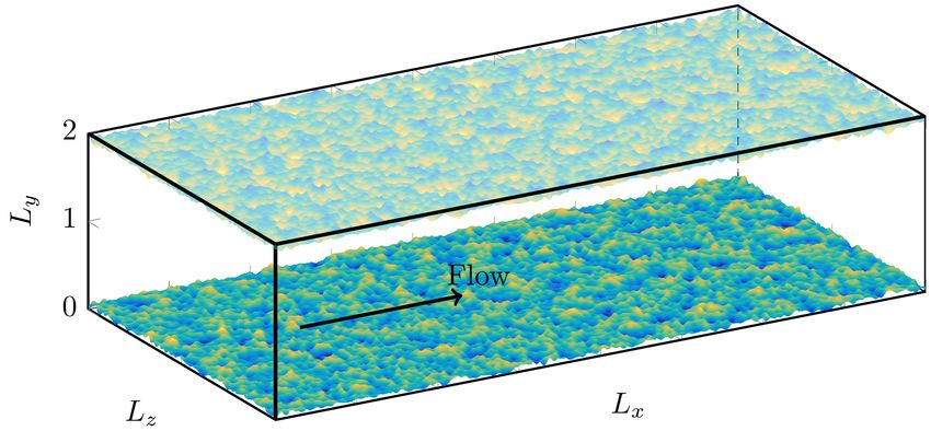
simulation domain is shown in figure 1, where x, y and z denote streamwise, wall-
normal and spanwise directions with respective velocity components u, v and w. The
roughness are mounted on both upper wall and lower wall. Channel half height, which is
the distance between the deepest trough in roughness and the centre plane of the channel,
is labeled as H and will be used to normalize the geometrical scales. The incompressible6 J. Yang, A. Stroh, D. Chung and P. Forooghi
Figure 1: Schematic representation of simulation domain with an example pseudo-realistic
surface mounted. Normalization of lengths with H is applied in the figure.
Navier-Stokes equations are solved using the pseudo-spectral solver SIMSON (Chevalier
et al. 2007), where wall-parallel directions are discretized in Fourier space, while in wall-
normal direction Chebyshev discretization is employed. Immersed Boundary Method
(IBM) based on Goldstein et al. (1993) is used to impose the no-slip boundary condition
on the roughness by introducing an external volume force field directly to the Navier-
Stokes equation. The presently used IBM implementation has been validated and used
in previous studies (Forooghi et al. 2018b; Vanderwel et al. 2019; Stroh et al. 2020).
The Navier-Stokes equation writes
∇⋅u = 0 , (2.1)
∂u 1 1
+ ∇ ⋅ (uu) = − ∇p + ν∇2 u − Px eˆx + fIBM , (2.2)
∂t ρ ρ
where u = (u,v,w)⊺ is the velocity vector and Px is the mean pressure gradient in the
flow direction added as a constant and uniform source term to the momentum equation
to drive the flow in the channel. Here p, eˆx , ρ, ν and fIBM are pressure fluctuation,
streamwise basis vector, density, kinematic viscosity and external body force term due
to IBM, respectively. Periodic boundary conditions are applied in the streamwise and
spanwise directions. No-slip boundary condition is applied on the rough√ walls. The friction
Reynolds number is defined as Reτ = uτ (H − kmd )/ν, where uτ = τw /ρ and τw = −Px ⋅
(H − kmd ) are the friction velocity and wall shear stress, respectively. Melt-down height
denoted by kmd is the mean roughness height measured from the deepest trough. Note
that we use (H − kmd ) which is the mean half cross section area divided by the channel
width – or arguably the effective channel half height – as the reference length scale in these
definitions. In total, four different values of Reτ in the range of 250-1000 are simulated in
the present work in order to be able to cover different regimes. The simulations designed
to study the effect of roughness topography are, however, performed mainly at Reτ = 500.
The simulation domain is discretized in equidistant grid in wall-parallel directions
while in wall-normal direction cosine stretching based on Chebyshev node distribution is
applied. The selection of grid size must take into consideration both flow and roughness
length scales. As reflected by Busse et al. (2015), each roughness wavelength should be
represented by multiple computational cells. Since we prescribe the PS in the roughness
generation approach, the range of present roughness wavelengths can be prescribed. Here
the smallest roughness wavelength, labeled as λ1 , is the crucial quantity for horizontal
grid resolution. Therefore, in the view of the present computational capacity, λ1 = 0.08H
is prescribed for the following simulations. Mesh independence study is carried out, fromDNS-based characterization of pseudo-random roughness in minimal channels 7
−2
⋅10
101
λ = 0.08H
λ = 0.8H
4
10−1
qref Ek (q)/krms
p = −2
Sk = 0
2
Sk = 0.48 Sk = −0.48 p = −1
PDF
2 −3
10
0 10−5
0 5 ⋅ 10−2 0.1 10−1 100 101 102
k/H q/qref
(a) PDF of roughness. (b) Normalized PS density with different p.
1
10 101
λ = 0.08H
λ = 0.08H
λ = 1.6H
λ = 0.8H
λ = 1.6H
λ = 0.8H
10−1 10−1
qref Ek (q)/krms
qref Ek (q)/krms
p = −2
p = −1
2
2
10−3 10−3
10−5 10−5
10−1 100 101 102 10−1 100 101 102
q/qref q/qref
(c) Normalized PS density with different λ0 , (d) Normalized PS density with different λ0 ,
p = −1. p = −2.
Figure 2: Statistical representation of the studied Roughness-In (b,c,d) wavenumber q
is normalized by the reference wavenumber qref = 2π/(0.8H). Vertical dashed lines are
high-pass filtering and low-pass filtering, corresponding to λ0 & λ1 respectively.
which the smallest roughness wavelength being resolved by 8-10 cells in each directions
is found adequate to obtain the converged double averaged velocity profile. Overall, the
grid size ∆+ < 5 in wall-parallel directions is proven to be appropriate through the mesh
independence test. In wall-normal directions, cosine stretching mesh is adopted for the
Chebychev discretization. It is also checked through the mesh independence test that for
present types of rough surfaces, a vertical cell number of 401 is sufficient in delivering a
converged result at highest Reτ ≈ 1000, thanks to the overresolving of roughness structure
by cosine stretching grid near wall.
2.3. Description of cases
Using the roughness generation algorithm introduced in section 2.1, multiple samples
are generated. In the present work, different types of PDF will be combined with power-
law PS, that is Ek (q) = C0 (∥q∥/q0 )p , where q is the wavenumber vector q = (qx ,qz )⊺ ,
q0 = 2π/λ0 is the smallest wavenumber corresponding to the largest in-plane length scale
λ0 , C0 is a constant to scale the roughness height, and p is the spectral slope of the power-
law PS. The overview of the configurations of PDF and PS is illustrated in figure 2. In
figure 2 (b,c,d) the PS density normalized by the r.m.s. of the roughness height are8 J. Yang, A. Stroh, D. Chung and P. Forooghi
compared in pairs. The upper and lower cutoff wavelength λ0 and λ1 are transformed to
cutoff wavenumbers q0 = 2π/λ0 and q1 = 2π/λ1 , which are represented by the red dashed
lines in figure 2 (b,c,d) on the left and right side of the figures respectively. As stated
in the previous section, the lower cutoff wavelength is related to the grid resolution
and a value of λ1 = 0.08H ≈ 8∆x ≈ 8∆z is applied for all roughness topographies in the
present work. With an isotropic roughness and a fixed λ1 , the PS is determined by two
remaining parameters, λ0 and p. In present work, two values of p (p = −1 and p = −2) are
examined, the PS of which are shown in figure 2 (b). For the selection of p values we
seek similarity to previous works (Anderson & Meneveau 2011; Barros et al. 2018; Nikora
et al. 2019). Moreover, two different upper cutoff wavelengths (λ0 = 0.8H and λ0 = 1.6H)
of the roughness PS are investigated. Power spectrum with λ0 = 0.8H and 1.6H with
identical slopes p are compared in figure 2(c,d), where wavenumber q is normalized by
referencing wavenumber qref = 2π/(0.8H)
Three types of PDFs with positive, zero and negative skewness are examined in the
present work. Covering a relatively large range of Sk is intended to ensure that the
results can be generalized to a wide spectrum of naturally occurring roughness in different
applications. The non-skewed roughness is described by a Gaussian distribution. For the
positively skewed roughness, Weibull distribution is used, which writes
f (k) = Kβ K k (K−1) e−(βk)
K
, (2.3)
where the parameters K and β can be used to adjust the standard deviation and skewness
of the distribution. The skewness is always adjusted to the value of 0.48. Similar to
the Gaussian distribution the Kurtosis of the Weibull distribution is always equal to
three. A negatively skewed PDF is obtained by flipping the PDF of a positively skewed
Weibull PDF. Here Sk = −0.48 is prescribed. In the present work, the 99% confidence
interval of roughness height PDF, k99 , is used as the characteristic size of roughness, i.e.
k = k99 . This measure is related to the standard deviation of the roughness, and hence
can be directly prescribed. We used a fixed value of k = 0.1H in all cases. Indeed, k is a
statistical measure of maximum peak-to-trough roughness size, which unlike the absolute
peak-to-trough size kt , is not deteriorated by extreme events. These types of PDFs are
illustrated in figure 2. Moreover, in order to avoid extreme high roughness elevations in
the simulations, roughness heights outside 1.2 times the 99% confidence interval of PDF
are excluded. Therefore, the peak-to-trough height kt = 0.12H for all roughness in the
present work. Combining the three types of PDF (with different values of Sk) with four
types of PS (two values of p and λ0 each) twelve different roughness topographies are
studied in the present work, which are summarized in table 1. Selected patches of all 12
roughness topographies on surfaces with size 2.4H ×0.8H, are displayed in figure 3. Above
each roughness map, the 1D roughness profile at z = 0.4H along streamwise direction is
shown.
For each roughness sample, simulations in full-span and minimal channels are carried
out. For minimal channels the spanwise size Lz is the main subject of the study. As the
log-layer flow structures are set by the spanwise dimension Lz (Flores & Jiménez 2010),
it is often most critical in terms of reducing the computational cost. The spanwise size
of the present minimal channels are designed to fulfil the three criteria set by inequality
(1.1). The first criterion (L+z > 100) stems from the fact that the computational domain
must accommodate the near wall cycle of turbulence and, unlike the other two criteria,
is independent of the roughness topography. The second criterion (L+z ≥ k̃ + /0.4) ensures
that roughness can be included in ’healthy turbulent’ zone under critical height. We
translate the criteria for a realistic roughness by replacing k̃ for the sinusoidal roughnessDNS-based characterization of pseudo-random roughness in minimal channels 9
k/H
k/H
0.12 0.12
0 0
z/H
z/H
0.4 0.4
(a) N 14 (b) N 24
0.8 0.8
0 0.6 1.2 1.8 2.4 0 0.6 1.2 1.8 2.4
k/H
k/H
0.12 0.12
0 0
z/H
z/H
0.4 0.4
(c) N 18 (d) N 28
0.8 0.8
0 0.6 1.2 1.8 2.4 0 0.6 1.2 1.8 2.4
k/H
k/H
0.12 0.12
0 0
z/H
z/H
0.4 0.4
(e) G14 (f) G24
0.8 0.8
0 0.6 1.2 1.8 2.4 0 0.6 1.2 1.8 2.4
k/H
k/H
0.12 0.12
0 0
z/H
z/H
0.4 0.4
(g) G18 (h) G28
0.8 0.8
0 0.6 1.2 1.8 2.4 0 0.6 1.2 1.8 2.4
k/H
k/H
0.12 0.12
0 0
z/H
z/H
0.4 0.4
(i) P 14 (j) P 24
0.8 0.8
0 0.6 1.2 1.8 2.4 0 0.6 1.2 1.8 2.4
k/H
k/H
0.12 0.12
0 0
z/H
z/H
0.4 0.4
(k) P 18 (l) P 28
0.8 0.8
0 0.6 1.2 1.8 2.4 0 0.6 1.2 1.8 2.4
x/H x/H
0 0.12 0 0.12
k/H k/H
Figure 3: Roughness maps with configuration M 1 − 500, color indicates height. 1D
roughness profile at z = 0.4H ( ) is shown above each roughness map. (a-d): negatively
skewed, (e-h): zero skewness, (i-l): positively skewed; left column: p = −1. right column,10 J. Yang, A. Stroh, D. Chung and P. Forooghi
by the characteristic roughness height k for any arbitrary roughness. The third criterion
states that the minimal channel should contain the roughness wavelength. However, for
the realistic surfaces a single characteristic wavelength is not naturally determined. A
conservative choice for this limit of the channel width can be the largest in-plane length
scale, which is λ0 in the present study. This ensures that all wavelengths present in the
roughness topography are included in the spanwise domain. Recalling the aim of reducing
the roughness simulation cost, however, we seek a less conservative choice, in which
some of the larger wavelengths are excluded. Particularly, for simulations of engineering
roughness, it is often impractical to include extremely large roughness scales. To formalize
our choice, we denote the largest spanwise wavelength that a domain can accommodate
as λ∗ , and calculate the portion of surface energy that larger wavelengths contribute to
the original roughness as
2π/λ∗
2π ∫2π/λ Ek (q)dq
Φ( ∗ ) = 2π/λ0 . (2.4)
λ ∫2π/λ0 Ek (q)dq
1
where λ is the discrete wavelength. If the spanwise domain size is λ∗ , the simulation
resolves a roughness with 1 − Φ portion of the original surface variance.
In the current research we examine a choice of spanwise channel size corresponding
to half the size of the largest length scale, i.e. λ0 /2. With the adopted power-law PS, it
leads to the values of 1 − Φ equal or larger than 90% for all samples under investigation.
Hence the third criterion is replaced by Lz ≥ λ1/2 , where λ1/2 = λ0 /2, which means that the
simulations resolve at least 90% of the original surface variance. The new criterion leads to
a minimum channel width of Lz = 0.8H for half of the investigated roughness topographies
(those with λ0 = 1.6H) and Lz = 0.4H for the other half (those with λ0 = 0.8H). We label
the minimal channels with the former (larger) and latter (smaller) spanwise sizes as M 1
and M 2, respectively. For roughness samples with λ0 = 0.8H simulations at both M 1
and M 2 channels are carried out. To complete the investigation, some simulation with
a further reduced channel size M 3 (Lz = 0.3H) are carried out. It is worth mentioning
that, since k = 0.1H holds for all topographies, M 1, M 2 and M 3 channels fulfill the
Lz ≥ k/0.4 criterion. For all simulation configurations the streamwise channel size Lx is
set according to the equation 1.2 once Lz is known.
Simulations are carried out at four different friction Reynolds numbers Reτ = 250,
500, 750 and 1000, at fixed k/H = 0.1, leading to k + = 25, 50, 75, and 100. However
the parametric study on roughness topography is only conducted at k + = 50. Apart
from minimal channel simulations, conventional full span channel simulations with the
size Lx × Ly × Lz = 8H × 2H × 4H, labeled as F , are also carried out for all roughness
topographies. For the two highest Reynolds numbers, however, such large simulations
are costly. Consequently, for these Reynolds numbers, the largest investigated channels
are smaller than the F channel (but still larger than M 1/M 2/M 3). These channels are
labeled as M 0. Table 2 summarizes the details of all simulations carried out for rough
channels. In order to provide a reference for determining the roughness function ∆U + ,
additional smooth-wall simulations are also performed in M 2, M 1 and F -sized channels
at Reτ = 500 (not shown in the table). Overall, each rough-wall simulation case is defined
by a combination of roughness topography and simulation configuration (channel size
and Reynolds number). Throughout the article, the following naming convention is usedDNS-based characterization of pseudo-random roughness in minimal channels 11
Topography Sk p λ0 /H ka /H kmd /H krms /H Lcorr
x /H Sf /S ESx
P 14 0.48 −1 0.8 0.017 0.046 0.0208 0.050 0.28 0.57
P 18 0.48 −1 1.6 0.017 0.046 0.0208 0.054 0.27 0.54
P 24 0.48 −2 0.8 0.017 0.046 0.0208 0.104 0.21 0.44
P 28 0.48 −2 1.6 0.017 0.046 0.0208 0.170 0.19 0.39
G14 0 −1 0.8 0.016 0.061 0.0200 0.050 0.27 0.54
G18 0 −1 1.6 0.016 0.061 0.0200 0.054 0.26 0.53
G24 0 −2 0.8 0.016 0.061 0.0200 0.104 0.20 0.43
G28 0 −2 1.6 0.016 0.061 0.0200 0.168 0.18 0.37
N 14 −0.48 −1 0.8 0.017 0.074 0.0208 0.050 0.28 0.57
N 18 −0.48 −1 1.6 0.017 0.074 0.0208 0.054 0.27 0.54
N 24 −0.48 −2 0.8 0.017 0.074 0.0208 0.104 0.21 0.44
N 28 −0.48 −2 1.6 0.017 0.074 0.0208 0.170 0.19 0.39
Table 1: Roughness topographical properties, where Sk = (1/krms 3
) ∫S (k − kmd )3 dS, ka =
(1/S) ∫S ∣k − kmd ∣dS is the mean absolute height deviation from the melt-down height
√
kmd = (1/S) ∫S kdS measured from deepest trough. krms = (1/S) ∫S (k − kmd )2 dS is the
standard deviation of the height function. Sf is the total frontal projected area of
the roughness. Lcorr
x refers to the length scale where the roughness auto-correlation in
streamwise direction drops under 0.2. ES = (1/S) ∫S ∣∂k/∂x∣dS represents the effective
slope.
to describe the cases:
Topography Simulation configuration
³¹¹ ¹ ¹ ¹ ¹ ¹ ¹ ¹ ¹ ¹ ¹ ¹ ¹ ¹ ¹ ¹ ¹ ¹ ¹ ¹ ¹ ¹ ¹ ¹ ¹ ¹ ¹ ·¹¹ ¹ ¹ ¹ ¹ ¹ ¹ ¹ ¹ ¹ ¹ ¹ ¹ ¹ ¹ ¹ ¹ ¹ ¹ ¹ ¹ ¹ ¹ ¹ ¹ ¹ ¹ µ ³¹¹ ¹ ¹ ¹ ¹ ¹ ¹ ¹ ¹ ¹ ¹ ¹ ¹ ¹ ¹ ¹ ¹ ¹· ¹ ¹ ¹ ¹ ¹ ¹ ¹ ¹ ¹ ¹ ¹ ¹ ¹ ¹ ¹ ¹ ¹ ¹µ
G 2 4 ∣ F − 500 . (2.5)
± ° ° ± ²
PDF −p 10λ1/2 /H ch. size 10k +
● The first character indicates the type of PDF; G for Gaussian distribution, P for
positively skewed (Sk ≈ 0.48), and N for negatively skewed (Sk ≈ −0.48).
● The second digit indicates the PS spectral slope; 1 for p = −1 and 2 for p = −2.
● The third digit represents the half of large cutoff wavelength λ1/2 , with which channel
width is determined; 4 for λ1/2 = 0.4H and 8 for λ1/2 = 0.8H.
● The following character(s) indicates the channel spanwise size; F for full channel
(Lz = 4H), M 1 and M 2 for the larger (Lz = 0.8H) and the smaller (Lz = 0.4H) minimal
channels, respectively. M 3 utilizes the spanwise width Lz = 0.3H. M 0 is introduced to
the cases which k + = 75 and 100 with Lz = 2H and 1H, respectively
● The last number denotes 10k + , or equivalently, Reτ .
2.4. Post-processing
The time-averaged flow field over a rough surface is heterogeneous in horizontal
directions. In order to analyze the one-dimensional mean profile of the flow, we apply
double averaging, as proposed by Finnigan & Shaw (2008). The double-averaged velocity
profile in the wall-normal direction ⟨u⟩(y) is obtained by averaging the time-averaged
velocity over wall-parallel directions, i.e.
1
⟨u⟩(y) = ∬ u(x,y,z)dxdz . (2.6)
S S12 J. Yang, A. Stroh, D. Chung and P. Forooghi
Topographies Configuration Reτ Lx /H Lz /H Nx Nz ∆+ x ∆+ z ∆+y,k FTT
G24 M 2 − 250 250 4.0 0.4 512 48 1.95 2.08 0.88 1200
G24 M 1 − 250 250 5.0 0.8 576 96 2.17 2.08 0.88 300
G24 F − 250 250 8.0 4.0 900 480 2.22 2.08 0.88 100
G24 M 3 − 500 500 2.0 0.3 256 48 3.91 3.13 1.74 1000
∗ ∗ 4 & G28 M 2 − 500 500 2.0 0.4 256 48 3.91 4.17 1.74 2000
all M 1 − 500 500 2.4 0.8 256 96 4.69 4.17 1.74 500
all F − 500 500 8.0 4.0 900 480 4.44 4.17 1.74 80
G24 M 2 − 750 750 1.4 0.4 288 96 3.65 3.13 2.59 1200
G24 M 1 − 750 750 2.4 0.8 480 160 3.75 3.75 2.59 300
G24 M 0 − 750 750 4.0 2.0 640 320 4.69 4.69 2.59 100
G24 M 2 − 1000 1000 1.2 0.4 288 96 4.17 4.17 3.53 500
G24 M 1 − 1000 1000 2.4 0.8 576 192 4.17 4.17 3.53 300
G24 M 0 − 1000 1000 3.0 1.0 720 240 4.17 4.17 3.53 100
Table 2: Summary of all simulation cases including roughness topography and simulation
configurations. For all cases Ly /H = 2,Ny = 401. Moreover, ∗ ∗ 4 indicates all roughness
topographies with λ1/2 = 0.4H, ∆+y,k indicates the grid size at the roughness height i.e.
y = 0.1H, flow through time (FTT= T Ub /Lx ) for statistics collection duration are shown
H
in the last column, where T is the total integral time, Ub = (1/Heff ) ∫0 U dy is the bulk
velocity, Heff = H − kmd .
where u(x,y,z) is time averaged streamwise velocity, S is the wall-normal projected
plan area (i.e. area of the corresponding smooth wall) and angular bracket ⟨⋅⟩ denotes
horizontal averaging. The double-averaged velocity profile ⟨u⟩(y) will be denoted as U
for simplicity. The time-averaged velocity field is obtained over a long enough period
of time. A minimum of 300 flow-through-times is used for the statistical integration in
minimal channels due to the bursting effect (Flores & Jiménez 2010). Initial transients
are removed from the statistical integration.
The influence of roughness on the mean flow is a downward shift in the inner-scaled
streamwise velocity profile relative to the smooth case (Schultz & Flack 2009). In other
words, as a result of the outer layer similarity (Townsend 1976), which states that outer-
layer flow is unaffected by the near wall events except for the effect due to the wall shear
stress, the downward shift of the velocity profile is approximately a constant value in the
logarithmic region and possibly beyond if the outer-flow geometry and Reynolds number
are matched. This downward velocity shift in the logarithmic region is referred to as
roughness function (Clauser 1956; Hama et al. 1954) ∆U + . Introducing the roughness
function to the logarithmic law of the wall (log-law hereafter), it writes
U+ = ln(y + − d+ ) + B − ∆U + .
1
(2.7)
κ
where κ ≈ 0.4 is the von Kármán constant, B ≈ 5.2 is the log-law intercept for the smooth
wall, d indicates the zero plane displacement which will be talked in detail in the following
section, and the superscript + indicates scaling in wall units. Based on the pioneering
work by Nikuradse (1933), the roughness function in the fully rough regime is a sole
function of the inner-scaled roughness size ks+ for the sand-grain roughness according to
∆U + = B − 8.48 + ln(ks+ ) .
1
(2.8)
κDNS-based characterization of pseudo-random roughness in minimal channels 13
Equation 2.8 is the basis for the definition of ‘equivalent’ sand-grain roughness (also
denoted by ks ) for an arbitrary roughness with the same roughness function.
In the present work, the roughness function ∆U + is calculated as the mean offset of
the inner-scaled mean velocity profile over the logarithmic layer for the cases with Reτ ≈
500. Since corresponding smooth channels in M 2, M 1 and F with matched Reτ ≈ 500
are available, this quantity is calculated by direct comparison to the smooth case. For
those cases with varied Reτ , further smooth channel simulations with matched Reτ are
required in order to derive the corresponding profile shift, which causes unfavourable
computational effort. Having in mind that log-law applies for minimal smooth channels
under critical height yc , a good approximation of velocity profile in log region of the
smooth channels can be drawn from the log-law, thus ∆U + is estimated by the velocity
shift at the critical height yc+ = 0.4 × L+z relative to the log-law U + = (1/κ)ln(y + ) + 5.2,
where κ = 0.4.
Finally it must be noted that, unlike a smooth channel, the origin of the wall-normal
coordinate for the log-law is not naturally defined for a rough wall. In this regard, Jackson
(1981) suggested use of moment centroid of the drag profile on rough surface as the virtual
origin for the logarithmic velocity profile. The definition of the virtual wall zero-plane
displacement d in present work follows Jackson’s method.
3. Results
3.1. Evaluation of minimal-channel simulations
In order to assess the applicability of the minimal channel, the simulations of the
roughness topography G24 with variation of channel size and k + are analyzed. The
comparison of different channel sizes at matched k + ≈ 50, i.e. the cases G24M 3 − 500,
G24M 2−500, G24M 1−500 and G24F −500, is discussed in section 3.1.1. This is followed
by the results for all different roughness topographies in section 3.1.2. As mentioned
before, the roughness generation process in the present research has a random nature, and
only statistical properties can be prescribed. To assess the effect of this randomness eight
independent simulations are carried out for eight random realizations of the roughness
topography G24 with k + ≈ 50. The results are presented in section 3.1.3. Finally in
section 3.1.4, one roughness topography is studied in a wide range of roughness Reynolds
numbers (k + = 25−100) in order to assess the prediction of the minimal channel in different
rough regimes. Here the roughness topography G24 is evaluated using minimal channels
M 2 and M 1 and (pseudo) full-span channels F /M 0.
3.1.1. Minimal channels with different spanwise sizes
The 3D schematic representations of minimal channels M 2 and M 1 as well as the
full span channel F used for simulations at k + ≈ 50 are shown in figure 4(a); M 3 is
not shown for simplicity. The hatched pattern indicates where the roughness is mounted.
Roughness topography G24 in the full-size simulation is shown in figure 4(b). For a direct
comparison, boundaries of minimal channels M 1 and M 2 are represented by the black
frames. The pseudo-random surfaces for each configuration is generated independently.
That is, for a specific topography, the surface height map in each simulation is unique,
but they all share identical statistical properties.
The inner-scaled velocity profiles obtained from roughness topography configuration
G24 with k + ≈ 50 are shown in figure 5(a). Colored dashed lines are the velocity profiles
extracted from smooth channel. The color indicates the size of channel. The critical
heights of minimal channels M 2 − 500 and M 1 − 500, i.e. yc+ = 0.4 × L+z = 80 and 160 are
illustrated by black vertical dashed lines in the figure, respectively. While the critical14 J. Yang, A. Stroh, D. Chung and P. Forooghi
0 M 2-500 0.12
M 1-500
Lz /H
2 2
Ly /H
1
0
0 8 F -500
6 4 0
2 4
4 0 2 0 2 4 6 8
Lz /H Lx /H Lx /H k/H
(a) Schematic simulation domain of F −
500, M 1 − 500 and M 2 − 500, hatch (b) Roughness map of G24F − 500
pattern represents roughness.
Figure 4: Comparison of channel sizes, black frames indicate minimal channels M 1 − 500
& M 2 − 500
30 8
critical height yc
G24M 3 − 500
G24M 2 − 500
6
20 G24M 1 − 500
G24F − 500 4
∆U +
U+
U + = ( 1 )log(y + ) + 5.2
0.4
2 critical height yc
10
G24M 2 − 500
0 G24M 1 − 500
G24F − 500
0 −2
100 101 102 100 101 102
(y − d)+ (y − d)+
(a) Mean velocity profile. ( : Rough, : (b) Velocity offset profile.
Smooth)
Figure 5: Simulation results of roughness type G24. Gray: M 3−500, red: M 2−500, green:
M 1 − 500, blue: F − 500. Red vertical line indicates roughness height measures from the
zero-plane displacement (k − d)+ .
height of M 3 − 500 i.e. yc+ = 60 is shown with gray vertical dashed line. It can be observed
from the figure, that minimal channel cases M 2−500 and M 1−500 successfully reproduce
the velocity profile of a conventional full-span channel under the critical height yc .
The velocity profiles deviate above the critical height yc due to the nature of minimal
channels. For G24M 3 − 500, however, some discrepancy of the profile can be observed
even under its critical height. In figure 5(b), the velocity offset profiles for F , M 1 and
M 2 channels are displayed. The velocity offset profiles are obtained by subtracting the
rough channel velocity profile from each corresponding smooth channel velocity profiles.
The velocity offset profile from minimal channels M 1, M 2 and full-span channel on the
right panel show excellent agreement. Consequently, it seems like the velocity offset is not
meaningfully affected by absence of the large wavelengths in spanwise direction with small
contribution to the roughness height power spectrum. This however does not hold for
channel M 3 where Φ(2π/Lz ) = 18%. A similar parameter study performed for roughness
topography G28 (not shown here) revealed that the velocity offset starts to deviate for
channel M 2 (Φ(2π/Lz ) = 16%). In both cases the deviation of the velocity profiles startsDNS-based characterization of pseudo-random roughness in minimal channels 15
∆U + d/k
Case F − 500 M 1 − 500 M 2 − 500 F − 500 M 1 − 500 M 2 − 500
P 14 7.33 7.28 7.35 0.81 0.81 0.82
P 24 6.99 6.86 6.92 0.78 0.77 0.80
P 18 7.23 7.34 - 0.81 0.81 -
P 28 6.57 6.87 - 0.76 0.76 -
G14 6.67 6.66 6.56 0.95 0.94 0.95
G24 6.30 6.39 6.43∗ 0.92 0.90 0.92∗
G18 6.56 6.59 - 0.95 0.95 -
G28 5.94 5.88 - 0.90 0.90 -
N 14 6.14 6.07 5.87 1.06 1.06 1.06
N 24 5.82 5.63 5.80 1.03 1.03 1.05
N 18 6.09 6.06 - 1.06 1.06 -
N 28 5.51 5.58 - 1.01 1.02 -
Table 3: Summary of roughness function ∆U + (left) and zero plane displacement d/k
(right) at k + ≈ 50, bold values are taken as the minimal channel results. ∗ : mean value
over 8 independent G24M 2 − 500s
when the contribution of excluded large wavelengths in the roughness height spectrum
is larger than 10%.
It is observed that due to the outer layer similarity the velocity offset in logarithmic
layer reaches approximately a constant value. In the present work, ∆U + of minimal
channels is obtained by averaging the mean velocity offset from each critical height yc+ to
the half of channel half-height 0.5H + , while full span channels is averaged in the region
y+ = 80 − 250. This gives ∆U + = 6.3 for case G24F − 500 and ∆U + = 6.4 and 6.2 for cases
G24M 1 − 500 and G24M 2 − 500, respectively.
3.1.2. Minimal channels for different roughness topographies
Applying the same analysis to all topographies at k + ≈ 50, roughness function ∆U +
are calculated and listed in table 3. It has to be mentioned that for case G24M 2 − 500,
multiple simulations are carried out for the purpose that will be discussed in section 3.1.3.
Therefore, roughness function of G24M 2 − 500 is the mean roughness function ∆U + over
G24M 2 − 500s and marked with ∗ . The value of ∆U + predicted by minimal channels
are compared with the prediction by full-span channels with matched topographical
property in figure 6. In this plot, the ±5% disagreement interval is illustrated by the green
+ +
shadow around ∆UMini /∆UFull = 1 (red line). Another key quantity widely discussed in
the framework of roughness studies is the zero-plane displacement d. Similar to ∆U + , d is
often used as input to roughness models, and therefore, its prediction is of practical value.
Motivated by that, in this section we also discuss predictions of d by minimal channels.
The value of d/k are also exhibited in the Table 3. Predicted zero-plane displacements d
in minimal channels are compared with full span channels in figure 7. It can be observed
that minimal channel predictions show excellent agreement with conventional full span
channel, the discrepancy lies under 5%. Consistent predictions of roughness function
∆U + indicate the capability of the minimal channels in reproducing roughness function
∆U + of the irregular pseudo-realistic roighness.16 J. Yang, A. Stroh, D. Chung and P. Forooghi
±5%
1
0.8 1.1
/∆UFull
+
1.05 ±5%
0.6
∆UMini
1
+
0.4
0.95
0.2 M 1 − 500
0.9
5.5 6 6.5 7 7.5
M 2 − 500
0
5 6 7 8
+
∆UFull
+
Figure 6: Roughness function predicted by minimal channels ∆UMini normalized with
+
full span channel prediction ∆UFull , ○: M 1 − 500, ◻: M 2 − 500. Green shadow indicates
+ +
prediction error interval of ±5% around ∆UMini /∆UFull =1 ( ). 99% confidence interval
is shown for case G24M 2 − 500
1.2
±5%
1
0.8 1.1
dMini /dFull
1.05 ±5%
0.6
1
0.4
0.95
0.2 M 1 − 500 0.9
M 2 − 500 40 45 50
0
35 40 45 50 55 60
dFull
Figure 7: Zero plane displacement predicted by minimal channels d+Mini normalized with
full span channel prediction d+Full , ○: M 1 − 500, ◻: M 2 − 500,
3.1.3. Effect of randomness
Due to the random nature of the roughness generation process, each generated rough-
ness is different from the other in a deterministic sense despite being statistically identical.
This randomness can be a source of uncertainty when pseudo-random roughness is used
as a surrogate of realistic roughness. As already observed in figure 6, the estimations of
∆U + in minimal channel show some scatter, which indicates a small uncertainty. The
present section is aimed to study randomness as a potential source of this uncertainty.
In the present section the prediction uncertainty caused by the random generation
process is studied. To this end, eight rough surfaces corresponding to the identical
topographical configuration G24 are generated independently. As a consequence, theDNS-based characterization of pseudo-random roughness in minimal channels 17
Case ∆U + d/k Case ∆U + d/k
No.1 6.46 0.92 No.5 6.64 0.92
No.2 6.44 0.91 No.6 6.23 0.92
No.3 6.59 0.91 No.7 6.58 0.92
No.4 6.20 0.92 No.8 6.30 0.91
Table 4: Roughness function and zero-plane displacement of G24M 2 − 500s. Mean
+
roughness function ∆U + G24M 2−500s = 6.43 comparing with ∆UG24F −500 = 6.30.
30
Reτ = 1000, k+ = 100 10 Moody (1944)
Reτ = 750, k+ = 75 Nikuradse (1933)
F /M 0
Reτ = 500, k+ = 50
Reτ = 250, k+ = 25
M1
20
M2
U + = ( 1 )log(y + ) + 5.2
0.4
∆U +
U+
5
10
0 0
0 1 2 3
10 10 10 10 101 102
+
(y − d) ks+
(a) Mean velocity profiles, line color (b) Roughness function. Data from Niku-
gradually changes from gray to black with radse’s uniform sand grain roughness and
increasing Reτ . Colebrook relation provide for industrial
( : F /M 0, : M 1, : M 2) pipes are added for comparison.
Figure 8: Simulations at different k + at fixed k/H; k + = 25 − 100.
roughness realization of each randomly generated surface is unique while the statistical
properties are nearly identical. To assess the effect of this randomness eight independent
simulations are run for eight random realizations of the roughness topography G24 with
k + ≈ 50 in minimal channel M 2. The computed values of ∆U + for all surfaces along
with the zero-plane displacement d/k are summarized in table 4. The averaged value of
roughness function over the eight G24M 2 − 500s is ∆U + G24M 2−500 = 6.43, while the 99%
uncertainty interval of all values is 0.31. The averaged ∆U + is shown in figure 6 along with
the 99% uncertainty interval. One can observe that the uncertainty bar well encompasses
the ∆U + in the full channel. This can be taken as an indication that minimal channel
prediction can converge to the exact value if the uncertainty due to randomness is ruled
out. Nevertheless, as stated before, the error associated with one random realization is
still considerably low. It is observed in figure 6 that the 99% confidence bar lies in the
green area, which is the 5% disagreement. Overall, it can be stated that DNS in minimal
channels with matched roughness statistics is an accurate tool for the prediction of ∆U +
of realistic roughness, apart from the small discrepancy, which is arguably linked to the
effect of randomness.18 J. Yang, A. Stroh, D. Chung and P. Forooghi
3.1.4. Minimal channels in transitionally and fully rough regimes
The values of ∆U + reported for the simulations with k + ≈ 50 suggest that the flow likely
lies in the border between transitionally and fully rough regimes. In order to ensure that
minimal channels deliver acceptable predictions in a wide range of scenarios including
both regimes, in this section we study one roughness topography (G24) in a range of
roughness Reynolds numbers k + ≈ 25 − 100. Both minimal channel simulations M 2 and
M 1 as well as large-span channel simulations F /M 0 are carried out. Simulation setups are
summarized in table 2. Mean velocity profiles are shown in figure 8(a), while roughness
functions ∆U + against ks+ are shown in figure 8(b). In figure 8(a) the value obtained
in minimal channels M 2 are plotted with dotted lines, M 1 are plotted with dashed
line while (pseudo) full span channels F /M 0 are represented by solid lines. One can
observe from figure 8(a) that each velocity profile deviates above the respective critical
height yc+ = 0.4 × L+z which are not shown for clarity. However outer-layer similarity can
be observed valid from the parallel velocity profile in the outer region. Here roughness
functions are obtained by calculating the velocity difference at each critical height relative
to the log-law U + = (1/0.4)log(y + ) + 5.2 . The calculated values of roughness function are
shown in figure 8(b) as a function of equivalent sand-grain size ks+ . Notably, the calculated
values of roughness function from both minimal and full channels show an excellent
agreement. Equivalent sand-grain roughness is calculated by fitting roughness function
to the asymptotic roughness function in fully rough regime as shown in figure 8(b). In
doing so we obtain an equivalent sand-grain roughness size of ks ≈ 1.05k for roughness
topography G24. It can be observed that ∆U + asymptotically approaches fully rough
regime at ∆U + ≈ 6. It is worth mentioning that each data point from figure 8(b) represents
unique realization of rough surface.
3.2. Roughness surface force
In the present simulations, IBM introduces a volume force within the solid area
imposing zero velocity and hence represents the action of pressure and viscous drag force.
One of the advantages of IBM is the explicit representation of localized hydrodynamic
force exerted by roughness (Chan-Braun et al. 2011), here referred to as ‘surface force’.
In this section, we investigate the link between the mean surface force distribution and
the roughness height distribution. Given the satisfactory performance of the minimal
channel demonstrated in section 3.1, the following analysis is carried out based on the
results achieved from minimal channels. Previous studies on irregular roughness report
that a certain range of roughness scales is dominant in generation of skin friction (Barros
et al. 2018). A deeper insight into the contribution of different roughness scales to the
drag force is the aim of this section. To this end, the local forcing map f(x,z) is obtained
by time-averaging the IBM force field fIBM (x,y,z,t) and integrating the force in wall-
normal direction y:
1 H T
f(x,z) = ∫ ∫ fIBM (x,y,z,t)dtdy, (3.1)
T 0 0
⊺
where f(x,z) = (fx ,fy ,fz ) is the force vector and fx , fy and fz are streamwise, wall-
normal and spanwise force component, respectively. The visualization of normalized
forcing map for all M 2 − 500 cases with their roughness distribution maps are shown in
figure 9. The entire set of surface force distributions show spanwise-elongated coherent
areas of negative forcing. Furthermore, force distributions in streamwise direction at
z = 0.2H are displayed for three cases N 24M 2−500 (negative skewness), G24M 2−500
(Gaussian) and P 24M 2−500 (positive skewness) in figure 10 along with the surface height
functions at the same location. In this figure, solid blue line represents the normalizedYou can also read