The road weather model RoadSurf (v6.60b) driven by the regional climate model HCLIM38: evaluation over Finland
←
→
Page content transcription
If your browser does not render page correctly, please read the page content below
Geosci. Model Dev., 12, 3481–3501, 2019
https://doi.org/10.5194/gmd-12-3481-2019
© Author(s) 2019. This work is distributed under
the Creative Commons Attribution 4.0 License.

The road weather model RoadSurf (v6.60b) driven by the regional
climate model HCLIM38: evaluation over Finland
Erika Toivonen1 , Marjo Hippi1 , Hannele Korhonen1 , Ari Laaksonen1,2 , Markku Kangas1 , and
Joni-Pekka Pietikäinen1,a
1 Finnish Meteorological Institute, Helsinki, Finland
2 Department  of Applied Physics, University of Eastern Finland, Kuopio, Finland
a now at: Climate Service Center Germany (GERICS), Hamburg, Germany

Correspondence: Erika Toivonen (erika.toivonen@fmi.fi) and Joni-Pekka Pietikäinen (joni-pekka.pietikaeinen@hzg.de)

Received: 19 December 2018 – Discussion started: 1 February 2019
Revised: 14 June 2019 – Accepted: 1 July 2019 – Published: 7 August 2019

Abstract. In this paper, we evaluate the skill of the road       can be used to study the impacts of climate change on road
weather model RoadSurf to reproduce present-day road             weather conditions in Finland by forcing RoadSurf with fu-
weather conditions in Finland. RoadSurf was driven by            ture climate projections from RCMs, such as HCLIM.
meteorological input data from cycle 38 of the high-
resolution regional climate model (RCM) HARMONIE-
Climate (HCLIM38) with ALARO physics (HCLIM38-
ALARO) and ERA-Interim forcing in the lateral boundaries.        1   Introduction
Simulated road surface temperatures and road surface con-
ditions were compared to observations between 2002 and           The road traffic sector is one field benefiting from im-
2014 at 25 road weather stations located in different parts      proved regional weather and climate information, especially
of Finland. The main characteristics of road weather condi-      at northern high latitudes. These regions do not only expe-
tions were accurately captured by RoadSurf in the study area.    rience frequent wintertime snow and ice conditions but also
For example, the model simulated road surface temperatures       rapidly changing road weather due to, for instance, the on-
with a mean monthly bias of − 0.3 ◦ C and mean absolute          set of snowfall (Juga et al., 2012) or during temperature
error of 0.9 ◦ C. The RoadSurf’s output bias most probably       variations around the freezing point (Kangas et al., 2015).
stemmed from the absence of road maintenance operations in       Systematic consideration of upcoming weather events helps
the model, such as snow plowing and salting, and the biases      the general public in their everyday commute and, further-
in the input meteorological data. The biases in the input data   more, road maintenance authorities to attend the roads in a
were most evident in northern parts of Finland, where the re-    cost-effective manner (Nurmi et al., 2013). In Finland, the
gional climate model HCLIM38-ALARO overestimated pre-            Finnish Meteorological Institute (FMI) has a duty to issue
cipitation and had a warm bias in near-surface air tempera-      warnings of hazardous traffic conditions to the general pub-
tures during the winter season. Moreover, the variability in     lic. To support this, the institute has developed a road weather
the biases of air temperature was found to explain on aver-      model, RoadSurf, which has been in operational use since
age 57 % of the variability in the biases of road surface tem-   2000 (Kangas et al., 2015).
perature. On the other hand, the absence of road maintenance        Road weather conditions are expected to be affected by
operations in the model might have affected RoadSurf’s abil-     ongoing anthropogenic climate change (e.g. Jaroszweski et
ity to simulate road surface conditions: the model tended to     al., 2014) throughout the inhabited northern high latitudes.
overestimate icy and snowy road surfaces and underestimate       This region is strongly impacted by the Arctic amplifica-
the occurrence of water on the road. However, the overall        tion of climate warming (Screen, 2014), which can clearly
good performance of RoadSurf implies that this approach          be seen, for instance, in the Finnish temperature records of
                                                                 the past 170 years (Mikkonen at al., 2015). The expected

Published by Copernicus Publications on behalf of the European Geosciences Union.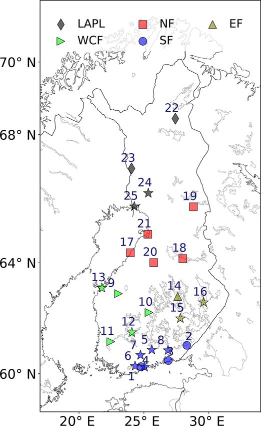
3482                                                             E. Toivonen et al.: The road weather model RoadSurf (v6.60b)

warmer and wetter future climate implies new challenges for           include reanalysis-driven RCM simulations at very high tem-
road maintenance and traffic safety, especially in the south-         poral resolutions, such as 1-hourly. Therefore, meteorologi-
ern parts of Finland: precipitation events are likely to shift to-    cal input data for RoadSurf are taken from HCLIM, which is
wards less snowfall and more frequent rain and sleet episodes         run for the years 2002–2014 with ALARO physics (Gerard,
(Räisänen, 2016). This kind of change in climate will de-             2007; Gerard et al., 2009; Piriou et al., 2007) at 12.5 km reso-
crease snowy road conditions but at the same time increase            lution. These HCLIM simulations are evaluated against stan-
the occurrence of wet road surfaces, which could lead to              dard meteorological datasets over Finland: E-OBS v19.0e
more frequently observed slippery and icy road conditions             (Cornes et al., 2018) and the ERA5 reanalysis product (C3S,
during the coldest times of a day, such as nighttime (Ander-          2017).
sson and Chapman, 2011a). Moreover, the events of temper-                In the previous studies, mainly NWP model outputs have
ature change around the freezing point might become more              been used to force RoadSurf. The simulated road weather
frequent in the northern parts of Finland (Makkonen et al.,           parameters, such as Troad , have been verified against obser-
2014), leading to an increased occurrence of black ice con-           vations over Finland (Karsisto et al., 2016) and the Nether-
ditions and making the roads more vulnerable to erosion.              lands (Karsisto et al., 2017). In addition, Kangas et al. (2015)
Therefore, policymakers and other stakeholders should have            have studied RoadSurf’s ability to simulate the amount of
access to credible regional climate projections that can pro-         water, snow, frost, and ice on the road (called storage terms in
vide a solid basis for informed impact assessments and adap-          RoadSurf) as well as road surface conditions and friction val-
tation measures in the road weather sector. A central tool for        ues, although only for two road weather stations in Finland.
producing such projections is high-resolution regional cli-           These studies have considered relatively short verification
mate models (RCMs).                                                   periods varying from 1 week to some months. In this paper,
   Although the impacts of climate change on road weather,            we concentrate on 13-year-long simulations of HCLIM and
safety, and design have been assessed in many studies (e.g.           HCLIM-driven RoadSurf. First, the performance of HCLIM
see Koetse and Rietveld, 2009), most of these studies have            is evaluated by comparing the model results with E-OBS
only considered relative changes in air temperature and pre-          v19.0e dataset of near-surface air temperature and precipi-
cipitation and related these to the possible impacts on the           tation and with ERA5 reanalysis for downwelling shortwave
roads (e.g. Andersson and Chapman, 2011a, b; Hambly et                and longwave radiation, total cloud fraction (clt), relative hu-
al., 2013; Hori et al., 2018; Makkonen et al., 2014). It would        midity, and wind speed. All of these parameters, excluding
be beneficial to study the climate change impacts on, for in-         clt, are used as inputs for RoadSurf. This comparison is fol-
stance, road surface temperatures (Troad ) or road surface con-       lowed by an evaluation of HCLIM-driven RoadSurf against
ditions using an approach in which these impacts can be ac-           observations at 25 road weather stations located in Finland.
cessed more directly. Furthermore, as slippery road condi-            The focus is on Troad but also the simulated road surface con-
tions, such as snowy or icy roads, are the major cause for the        ditions and storage terms are compared to the observations.
wintertime and weather-related road accidents in Fennoscan-           In addition, this study investigates the role of the biases in
dia (Andersson and Chapman, 2011b; Malin et al., 2019;                the HCLIM data on the biases in road surface temperature
Salli et al., 2008), it is essential to estimate how frequently       produced by HCLIM-driven RoadSurf.
these conditions will occur in the future.
   The main goal of this paper is to evaluate the skill
of RoadSurf to reproduce present-day road weather con-                2     Models and data
ditions in Finland when driven by a state-of-the-art high-
resolution RCM, cycle 38 of the HIRLAM-ALADIN Re-                     2.1     Models
gional Mesoscale Operational Numerical Weather Prediction
(NWP) In Europe (HARMONIE) Climate (HCLIM) (Lind-                     2.1.1    HARMONIE-Climate (HCLIM)
stedt et al., 2015). HCLIM is forced by the ERA-Interim
reanalysis product (Dee et al., 2011) in the lateral bound-           HARMONIE is a seamless NWP model framework devel-
aries since it is a standard procedure to carry out evaluation        oped in collaboration with several European national mete-
experiments using the (close to) perfect boundary settings            orological services (Bengtsson et al., 2017). The nonhydro-
in RCMs (e.g. Kotlarski et al., 2014). This is the first time         static and spectral dynamical cores in HARMONIE are pro-
that such a modeling chain is evaluated, and therefore this           vided by ALADIN–NH (Bénard et al., 2010), which solves
evaluation is needed in order to build and study future sce-          the fully compressible Euler equations using a two-time
narios of road weather in this area with higher confidence.           level, semi-implicit, semi-Lagrangian discretization on an
Although high-resolution climate projections for Europe are           Arakawa A grid. This study applied a model setup using the
currently available through the EURO-CORDEX interna-                  cy38h1 climate model version of HARMONIE with ALARO
tional climate downscaling initiative that provides RCM data          physics (HCLIM38-ALARO hereafter), as mentioned be-
at 50 km (EUR-44) and 12.5 km (EUR-11) resolutions (Jacob             fore; a hydrostatic version of the dynamical core; and a time
et al., 2014), the EURO-CORDEX dataset does not publicly              step of 300 s. The HCLIM38-ALARO version used in this

Geosci. Model Dev., 12, 3481–3501, 2019                                                 www.geosci-model-dev.net/12/3481/2019/
E. Toivonen et al.: The road weather model RoadSurf (v6.60b)                                                                      3483

                                                                        melting, and evaporation, are parameterized. The model esti-
                                                                        mates road surface friction using a numerical statistical equa-
                                                                        tion (Juga et al., 2013). RoadSurf assumes a flat horizontal
                                                                        surface which does not have any shading elements, such as
                                                                        trees. However, topography in general is taken into account
                                                                        implicitly through the input data. Thermodynamic properties
                                                                        of the road surface and ground are assumed to be similar
                                                                        for all simulated points, and the first two layers of the sur-
                                                                        face are always described as asphalt. In addition, the effect
                                                                        of traffic on the road surface is included: the model assumes
                                                                        that traffic packs some part of the snow into ice, whereas
                                                                        the remaining part is assumed to be blown away from the
                                                                        road. However, the model does not take into account winter-
                                                                        time road maintenance operations, such as salting and snow
                                                                        plowing, because RoadSurf is also used to plan and optimize
                                                                        these maintenance actions. The absence of road maintenance
Figure 1. The HCLIM38-ALARO model domain and topography at
                                                                        in the model implies that there will be unavoidable discrepan-
12.5 km × 12.5 km grid resolution. Colored overlays depict the re-      cies when comparing the modeled and observed road weather
gions that are evaluated in more detail. The transparent areas depict   conditions.
the model’s 8-point wide relaxation zone.                                  As inputs, RoadSurf needs near-surface air temperature
                                                                        (Tair ), near-surface relative humidity (RH), 10 m wind speed
                                                                        (WS), precipitation (Pr); and downwelling shortwave (SWd )
study includes a lake model, FLake (Mironov, 2008; Mironov              and longwave (LWd ) radiation. In the operational use, the
et al., 2010), and a surface parameterization framework, sur-           model employs observations from road weather stations, me-
face externalisée (SURFEX) (Masson et al., 2013). A more                teorological SYNOP (surface synoptic observations) weather
thorough description of HCLIM can be found in Lindstedt et              stations, and radar precipitation networks to initialize road
al. (2015) and cycle 38 of HCLIM is described in more detail            conditions while the road weather is predicted for the up-
in Belušić et al. (2019).                                              coming days utilizing forecasts produced by NWP models.
   For this study, HCLIM38-ALARO was run from Jan-                      In this study, we did not include any forecasted periods im-
uary 2002 to December 2014 (years 2000 and 2001 as a                    plying that no in situ observations were used to initialize and
spinup) over the Fennoscandian domain (151 × 181 grid                   force RoadSurf. Instead, RoadSurf was modified so that it
boxes) with 12.5 km × 12.5 km horizontal grid resolution                utilizes the RCM data, in this case the output of reanalysis-
and 65 vertical layers. Figure 1 depicts the HCLIM38-                   driven HCLIM38-ALARO. In addition to the abovemen-
ALARO simulated domain along with the model’s 8-point                   tioned inputs needed by RoadSurf, we utilized the bottom
wide relaxation zone as well as the regions of Finland that             layer ground temperature (at the depth of 4.28 m) produced
are analyzed in more detail in this study. The sea surface              by HCLIM38-ALARO. Using the simulated ground temper-
(sea-surface temperature and sea-ice concentration) and lat-            ature instead of the climatological one was motivated by the
eral boundary conditions of HCLIM38-ALARO were taken                    fact that although in the original RoadSurf version this tem-
from ERA-Interim reanalysis (Dee et al., 2011) every 6 h. In            perature is assumed to vary sinusoidally, it is estimated by
this study, the HCLIM38-ALARO output parameters were                    an equation in which some of the parameter values are based
produced every full hour and were used to force RoadSurf                on measurements retrieved from only one FMI observatory
offline.                                                                located in Southern Finland. RoadSurf’s main outputs are
                                                                        Troad and a traffic index describing driving conditions, but the
2.1.2   RoadSurf                                                        model produces also surface friction; prevailing road condi-
                                                                        tions; and the sizes of water, snow, and ice storages on the
The road weather model RoadSurf used in this study is a 1-              road. RoadSurf divides the road surfaces into eight classes:
D model based on solving the energy balance at the ground               dry, damp, wet, wet snow, frosty, partly icy, icy, and dry snow.
surface. This study employed the RoadSurf version 6.60b,                This classification is mainly based on the storage terms and
which is the operational version of the FMI’s research de-              Troad . The model physics of RoadSurf is described in more
partment with slight I/O changes made for this study. The               detail in Kangas et al. (2015).
model takes into account the conditions at the road surface
and beneath it, and calculates the vertical heat transfer into
the ground as well as at the interface of ground and atmo-
sphere. Hydrological processes, such as accumulation of rain
and snow, run-off from the surface, sublimation, freezing,

www.geosci-model-dev.net/12/3481/2019/                                                    Geosci. Model Dev., 12, 3481–3501, 2019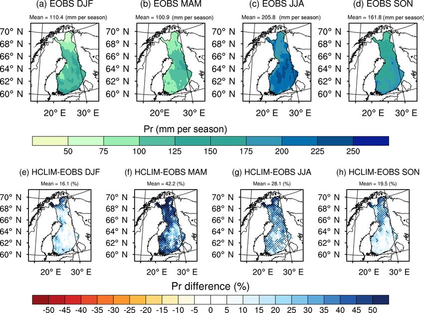
3484                                                          E. Toivonen et al.: The road weather model RoadSurf (v6.60b)

2.2     Evaluation data                                            2.2.2   ERA5 reanalysis product

2.2.1    E-OBS dataset of gridded daily precipitation and          Reanalysis is a scientific method that is based on a combi-
         near-surface air temperature                              nation of data assimilation and numerical models. The fifth
                                                                   generation of the ECMWF’s atmospheric reanalyses of the
The HCLIM38-ALARO simulated daily precipitation and                global climate, ERA5, provides hourly atmospheric data esti-
near-surface air temperatures were compared with the E-            mates at a horizontal grid resolution of approximately 30 km
OBS dataset, version 19.0e (Cornes et al., 2018), which con-       (Hersbach et al., 2018). This product was created using 4D-
sists of daily precipitation and 2 m air temperature (daily        Var data assimilation and the ECMWF’s Integrated Forecast
minimum, mean, and maximum) data retrieved from stations           System (IFS) cycle 41r2 that was used as the operational
located in Europe. The data are available as a regular grid        medium-range forecasting system in 2016. The model in-
which covers the pan-European domain with a resolution of          cludes 137 levels in the vertical reaching to 1 Pa. Overall,
0.11◦ (approximately 12 km). This E-OBS version, 19.0e,            ERA5 assimilates more observations compared to the ERA-
consists of a 100-member ensemble of realizations for each         Interim reanalysis product. However, it is good to note that
daily field. We utilized ensemble means that can be taken as       the ERA5 dataset is based on a model that is assimilating
grid box averages (Cornes et al., 2018) and that are compa-        observations and thus the dataset is prone to similar model
rable to the best guess grid in the earlier versions of E-OBS      deficiencies as other weather and climate models.
(Haylock et al., 2008).                                               We utilized the monthly means of daily means for clt,
   In general, gridded datasets, such as E-OBS, include un-        SWd , LWd , 10 m WS, and near-surface RH to evaluate
certainties due to the use of point measurements (e.g. rain        the performance of HCLIM38-ALARO. Monthly means of
gauges) and interpolation procedures. For example, the un-         daily-mean RH were computed employing the ERA5 product
dercatch of precipitation can lead to high biases especially       of hourly near-surface Tair and dew point temperature (Tdew )
in winter at high latitudes as well as in the areas of rough       (RH = 100×es (Tdew )/es (Tair )) as RH is not archived directly
topography (e.g. Prein and Gobiet, 2017). These undercatch         in the ERA5 dataset. Saturation vapor pressure (es ) was cal-
errors are typically between 3 % and 20 % for rainfall and up      culated based on the Magnus formula and with respect to
to 40 % (for shielded) or even up to 80 % (for nonshielded         water (WMO, 2008). Modeled near-surface RH was directly
gauges) for snow (Goodison et al., 1998). Moreover, the ac-        available and used as such.
curacy and success of the E-OBS dataset depend on the num-            Similarly to the comparison with the E-OBS data, the eval-
ber of stations used in the gridding process (Cornes et al.,       uation was carried out using the coarsest grid resolution by
2018): the sparse station density can introduce errors into the    remapping HCLIM38-ALARO model results into the ERA5
gridded dataset (e.g. Prein and Gobiet, 2017). For Finland,        grid using bilinear interpolation. Again, a standard Student’s
the station density is sparser in the northern parts compared      t test at a 95 % confidence level was used to assess the signif-
to the south (Fig. S1 in the Supplement). Although these ob-       icance of the differences between the modeled and observed
servational uncertainties are not in the scope of this study,      monthly averages (in the case of clt, LWd , WS, and RH) or
they should be kept in mind when analyzing the results.            seasonal averages (in the case of SWd ).
   The comparison of modeled and observed data was per-
formed using the coarsest grid resolution. The HCLIM38-            2.2.3   Road weather stations
ALARO model results covering Finland were thus compared
with E-OBS by remapping the E-OBS values into the grid of          The results obtained by the RoadSurf-HCLIM configuration
HCLIM38-ALARO: temperature data by using bilinear and              were compared with observations retrieved from 25 road
precipitation data by using first-order conservative remap-        weather stations located in different regions of Finland. Ta-
ping. The areas with a lake fraction greater than or equal to      ble 1 describes the features of these stations, such as location,
0.5 have been excluded from the analysis because E-OBS             surrounding characteristics, road maintenance class, and the
data over the lakes are based on the interpolation of the mea-     monthly average air temperatures, during October and April
surements over land. Moreover, the modeled 2 m air tem-            from 2002 to 2014. Stations 1–8 are located in Southern Fin-
perature values have been corrected using a lapse rate of          land, stations 9–13 in Western and Central Finland, stations
0.0064 ◦ C m−1 to account for the differences between the          14–16 in Eastern Finland, stations 17–21 in Northern Fin-
orography in the E-OBS dataset and the model. A standard           land, and stations 22–25 in Lapland (Fig. 2). The model grid
Student’s t test at a 95 % confidence level was used to assess     cell closest to each of these stations was selected for evalu-
the significance of the differences between the modeled and        ation. However, it needs to be noted that the model output
observed monthly averages (in the case of temperature) or          represents an areal average over the whole model grid cell,
monthly sums (in the case of precipitation).                       whereas the road weather observations are point measure-
                                                                   ments.
                                                                      The road weather stations are equipped with the Vaisala
                                                                   ROSA road weather package and Vaisala DRS511 sensors

Geosci. Model Dev., 12, 3481–3501, 2019                                              www.geosci-model-dev.net/12/3481/2019/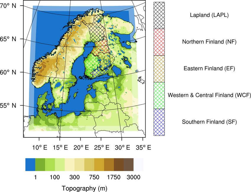
Table 1. Descriptions of the road weather stations with the mean observed air temperatures (◦ C) for the months between October and April in 2002–2014. The stations with an optical
sensor are marked with an asterisk (*). The road orientation is defined in parenthesis. As an example, SE–NW means that the orientation of the road is from southeast to northwest. The
maintenance classes are described in Appendix A (class 1 means high maintenance and class 4 low maintenance).
Region Number Station Coordinates Surrounding characteristics Maintenance Mean T Mean T Mean T Mean T Mean T Mean T Mean T
name and road class (◦ C) (◦ C) (◦ C) (◦ C) (◦ C) (◦ C) (◦ C)
orientation October November December January February March April
Southern 1 Askisto 60.27◦ N, 24.77◦ E Open area and a few trees (E–W) 1 5.8 1.6 −2.0 −5.1 −5.5 −2.1 4.4
Finland 2 Lappeenranta 61.07◦ N, 28.31◦ E Open area and trees nearby (SW–NE) 2 4.3 0.0 −4.4 −7.6 −7.6 −3.3 3.6
3 Sutela 60.50◦ N, 26.88◦ E Open area and a few trees, river nearby (E–W) 2 5.6 1.1 −2.4 −5.5 −7.0 −2.7 3.8
www.geosci-model-dev.net/12/3481/2019/
4* Jakomäki 60.25◦ N, 25.06◦ E Open area and trees on both sides of the road (SW–NE) 1 6.1 1.8 −1.5 −4.4 −5.2 −1.7 4.4
5* Lahti 60.91◦ N, 25.61◦ E Open area (SW–NE) 1 4.7 0.8 −3.2 −6.5 −6.6 −2.6 4.0
6* Palojärvi 60.29◦ N, 24.32◦ E Open area and a few trees, trees on the opposite side 1 5.1 1.2 −2.5 −5.5 −5.8 −2.6 3.8
(E–W)
7* Riihimäki 60.71◦ N, 24.74◦ E Empty lane between the road (SE–NW) 1 4.8 0.4 −3.9 −6.1 −5.9 −2.4 4.2
8* Utti 60.89◦ N, 26.86◦ E Open area, a few trees, and trees on the opposite side of 2 4.2 0.3 −3.8 −7.1 −7.1 −2.9 3.7
the road (E–W)
Western & 9 Lapua 62.94◦ N, 23.04◦ E Open area and trees on both sides of the road (S–N) 2 3.8 −0.3 −4.0 −6.9 −6.6 −3.0 3.5
Central Finland 10 Petäjävesi 62.27◦ N, 25.39◦ E Open area, a few trees, and trees on the opposite side of 3 3.5 −0.7 −5.0 −8.2 −8.2 −4.2 2.7
the road (E–W)
E. Toivonen et al.: The road weather model RoadSurf (v6.60b)
11 Seppälänahde 61.21◦ N, 22.45◦ E Open area and trees on both sides of the road (SE–NW) 2 4.9 0.9 −2.8 −5.9 −5.7 −2.3 4.0
12* Suinula 61.55◦ N, 24.07◦ E Open area and trees on both sides of the road (SW–NE) 2 4.3 0.2 −4.0 −7.0 −7.1 −3.5 3.3
13* Vaasa 63.14◦ N, 21.76◦ E Open area and trees on both sides of the road (SW–NE) 2 4.6 0.3 −3.6 −5.7 −6.6 −3.2 2.9
Eastern 14 Kuopio E 62.84◦ N, 27.61◦ E Empty lane between the road (S–N) 1 3.6 −0.7 −5.2 −8.9 −8.8 −4.1 2.8
Finland 15* Puunkolo 62.06◦ N, 27.81◦ E Open area, a few trees, and trees on the opposite side of 3 3.6 −0.9 −5.6 −8.7 −8.7 −4.3 2.6
the road (S–N)
16* Ylämylly 62.63◦ N, 29.60◦ E Open area (SW–NE) 2 3.8 −1.0 −5.7 −9.1 −9.2 −4.5 2.3
Northern 17 Kalajoki 64.34◦ N, 23.96◦ E Open area and trees on both sides of the road (SW–NE) 3 4.3 −0.1 −3.8 −7.1 −7.3 −4.1 1.8
Finland 18 Korholanmäki 64.14◦ N, 28.00◦ E A few trees and trees on the opposite side of the road 3 2.3 −2.5 −6.6 −9.6 −9.4 −4.9 2.0
(SE–NW)
19 Kuolio 65.83◦ N, 28.82◦ E Open area (SW–NE) 4 0.9 −4.4 −8.6 −12.2 −11.6 −7.7 −0.5
20 Kärsämäki 64.01◦ N, 25.76◦ E Open area and trees on the opposite side of the road (S– 3 2.7 −1.8 −6.1 −9.4 −9.0 −4.7 2.1
N)
21 Ouluntulli 64.95◦ N, 25.53◦ E Open area and a small hill nearby (SE–NW) 1 3.2 −1.4 −5.6 −9.1 −8.8 −5.1 2.0
Lapland 22 Saariselkä 68.46◦ N, 27.43◦ E Open area (SW–NE) 4 −0.5 −6.0 −8.4 −11.2 −11.2 −7.2 −1.4
23 Sieppijärvi 67.00◦ N, 24.05◦ E Open area and trees on both sides of the road (S–N) 4 0.1 −6.7 −9.1 −12.8 −11.9 −6.9 0.5
24* Jaatila 66.25◦ N, 25.34◦ E Open area and trees on both sides of the road (SW–NE) 3 1.6 −4.0 −7.4 −11.2 −10.6 −6.2 1.0
25* Kyläjoki 65.84◦ N, 24.26◦ E Open area, at the start of an overpass (E–W) 2 2.6 −2.6 −6.1 −9.8 −9.7 −5.6 0.8
Geosci. Model Dev., 12, 3481–3501, 2019
3485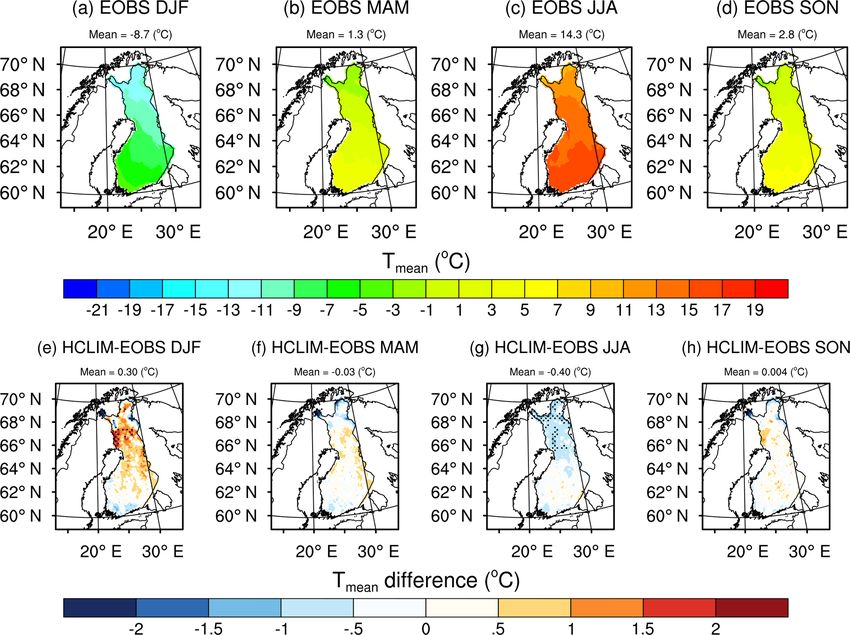
3486                                                              E. Toivonen et al.: The road weather model RoadSurf (v6.60b)

                                                                       gether considering that observations did not have a directly
                                                                       comparable class for wet snow. In addition, observations
                                                                       do not include a “partly icy” class which is defined in the
                                                                       model. Therefore, these divergent definitions of road condi-
                                                                       tion classes might cause some discrepancies when comparing
                                                                       the modeled and observed road conditions.

                                                                       3     Results and discussion

                                                                       3.1     Evaluation of HCLIM38-ALARO

                                                                       3.1.1    Mean near-surface air temperature

                                                                       The HCLIM38-ALARO model accurately captured the daily
                                                                       and seasonal mean 2 m air temperatures (Tair ) over Finland
                                                                       between 2002 and 2014. This is confirmed by Fig. S2 which
                                                                       illustrates the probability density functions (PDF) of the
                                                                       daily Tair for the observations and model during different sea-
                                                                       sons over all the grid points falling over Finland. Overall, the
                                                                       general shapes of Tair distributions were correctly reproduced
                                                                       by HCLIM38-ALARO with the largest deviations found in
                                                                       the winter season (December–February).
                                                                          Also, the multiyear mean seasonal Tair was well captured
                                                                       by HCLIM38-ALARO. Figure 3 shows the seasonal means
                                                                       from E-OBS as well as the mean biases in the HCLIM38-
                                                                       ALARO simulated mean seasonal Tair with a reference to
                                                                       E-OBS. The stippled areas depict significant differences in-
Figure 2. Locations of road weather stations used in this study. The   dicated by the Student’s t test (p < 0.05). The mean biases
numbers refer to Table 1. The stations with an additional optical      averaged over Finland were slightly positive in the autumn
sensor are marked as stars. SF stands for Southern Finland, WCF        and winter (September–February) and negative in the spring
for Western and Central Finland, EF for Eastern Finland, NF for        and summer (March–August). The autumn season had the
Northern Finland, and LAPL for Lapland.                                smallest domain-averaged bias of 0.004 ◦ C and the summer
                                                                       season the highest domain-averaged bias of −0.40 ◦ C. The
                                                                       biases were statistically significant mainly over the north-
(Vaisala, 2018a), which are installed in the road surface.             ern parts of Finland where the model had an enhanced warm
Thirteen of the selected stations included also the Vaisala            bias in the winter and cold bias in the summer. These bi-
DSC111 optical sensor (Vaisala, 2018b), which provides in-             ases might partly be caused by the lower station density in
formation on, for instance, water, snow, and ice storages on           the northernmost domain, which might decrease the accu-
the road. Two of the stations with an optical sensor had a             racy of the E-OBS data. On the other hand, the model was in
large amount of missing data and, therefore, only 11 of them           good agreement with the observations during the spring and
were included in this study. This study employs the road               autumn when most of the differences were not statistically
surface temperature and the information on the road surface            significant.
classes provided by the ROSA stations and the storage terms               It is good to note that Lindstedt et al. (2015) encoun-
provided by the stations with the additional optical sensors.          tered similar warm biases in their HCLIM-ALARO simu-
Data availability was on average 79 % (range 57 %–91 %) at             lations with cycle 36 over Sweden during the wintertime
ROSA stations and 32 % (range 18 %–38 %) at stations with              and they suggested it might originate from the nonprognos-
the optical sensor during the study period of 2002–2014.               tic lake surface temperatures. A prognostic lake model was
   The classification of observed and modeled road surface             included in the model version used in this study, and thus
conditions differ slightly. For example, the observations in-          the warm bias might have stemmed from other reasons, such
cluded “damp and salty” as well as “wet and salty” road sur-           as from SURFEX’s own features or the possible biases in
face classes. These classes were combined with “damp” and              ERA-Interim’s sea-surface temperatures or sea-ice concen-
“wet”, respectively because RoadSurf does not include in-              trations that are used to force the sea surface in HCLIM. On
formation on salting of the roads. The “wet snow” and “dry             the other hand, the HCLIM38-ALARO results for mean sea-
snow” classes provided by RoadSurf were also grouped to-               sonal Tair were in agreement with EURO-CORDEX RCMs

Geosci. Model Dev., 12, 3481–3501, 2019                                                  www.geosci-model-dev.net/12/3481/2019/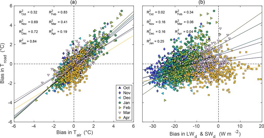
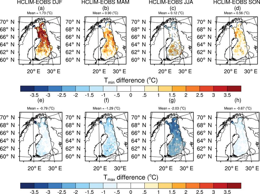
E. Toivonen et al.: The road weather model RoadSurf (v6.60b)                                                                  3487

Figure 3. (a–d) The reference values of mean near-surface air temperatures (Tmean ) from E-OBS data and (e–h) the biases of HCLIM38-
ALARO modeled Tmean with a reference to E-OBS. The seasonal means were calculated over the whole model domain for the time period
of January 2002–December 2014. Stippled areas represent statistically significant differences with p values < 0.05.

that were run at 12.5 km grid resolution. For instance, Kot-
larski et al. (2014) showed that some of the ERA-Interim-
driven EURO-CORDEX RCMs had a warm (cold) bias es-
pecially over the northern parts of Finland during the winter
(summer). However, a more detailed analysis of the causes
of the model biases is out of the scope of this study.
   Figure 4 demonstrates that the mean monthly biases in the
simulated daily Tair with a reference to the E-OBS dataset
were generally between ±1 ◦ C when the biases were av-
eraged over different regions of Finland for the period of
2002–2014. The highest positive biases occurred in the win-
ter season and the highest negative biases in the summer
as discussed before. However, some regional differences             Figure 4. The monthly mean biases of simulated near-surface air
were apparent. For example, in Southern Finland, the biases         temperature averaged over Southern Finland (SF), Western and
were mainly negative during the autumn and winter months            Central Finland (WCF), Eastern Finland (EF), Northern Finland
(October–February). Similarly, the biases were negative at          (NF), Lapland (LAPL), and the whole of Finland (ALL) in 2002–
the beginning of the winter season in Western and Cen-              2014 with a reference to E-OBS.
tral Finland but the biases during the late winter and early
spring season were positive as opposed to the negative bi-
ases in Southern Finland (excluding March when the bias             3.1.2   Minimum and maximum near-surface air
in Southern Finland was also positive). In Eastern Finland,                 temperature and percentiles of mean temperature
the mean biases resembled Western and Central Finland but
were slightly higher for every month except for July, Novem-        Similarly to the mean near-surface Tair , we assessed the
ber, and December. The monthly biases were even higher in           differences between the observed and modeled daily PDFs
Northern Finland and Lapland compared to the other parts            as well as the multiyear seasonal means of daily mini-
of Finland. In the northernmost areas, the biases were mostly       mum and maximum near-surface temperatures (Tair,min and
positive during the autumn and winter seasons and negative          Tair,max , respectively) in 2002–2014 over Finland. Again,
during the spring and summer.                                       the PDFs of both Tair,min and Tair,max were adequately rep-

www.geosci-model-dev.net/12/3481/2019/                                                 Geosci. Model Dev., 12, 3481–3501, 2019
3488                                                           E. Toivonen et al.: The road weather model RoadSurf (v6.60b)

Figure 5. The biases in the simulated seasonal means of (a–d) minimum near-surface air temperature (Tmin ) and (e–h) maximum near-
surface air temperature (Tmax ) with a reference to E-OBS. The seasonal mean biases were calculated over Finland for the time period of
January 2002–December 2014. Stippled areas represent statistically significant differences with p values < 0.05.

resented in HCLIM38-ALARO with the largest deviations                 appeared in the summer with a maximum domain-averaged
in the winter season (not shown). Figure 5 shows that the             difference of −2.2 ◦ C.
multiyear seasonal means of Tair,min were mainly overes-
timated and, contrarily, Tair,max underestimated. The stip-           3.1.3   Precipitation and wet-day frequency
pled areas in Fig. 5 depict significant differences pointed out
by the Student’s t test (p < 0.05). The differences between           Also multiyear mean seasonal precipitation sums were reli-
HCLIM38-ALARO and E-OBS were significant mainly in                    ably simulated by HCLIM38-ALARO although slight over-
the winter and summer season for Tair,min with the largest            estimation was evident. Figure 6 depicts both observed mul-
domain-averaged difference of 1.73 ◦ C found in the winter.           tiyear mean seasonal precipitation sums from the E-OBS
For Tair,max , the differences were significant mostly in the         dataset over Finland in 2002–2014 as well as the differ-
summer with also the largest domain-averaged difference of            ences between HCLIM38-ALARO with a reference to E-
−2.03 ◦ C occurring in the summertime.                                OBS. Similarly to the figures shown before, the stippled areas
   In addition to daily minimum and maximum temperatures,             represent significant differences confirmed by the Student’s
the differences in the 5th, 25th, 75th, and 95th percentiles of       t test (p < 0.05). Overall, precipitation was overestimated
the daily-mean Tair between the model and observations were           rather than underestimated throughout the year. The biases
computed for different seasons (Fig. S5). The spatial differ-         were the smallest in the winter with a domain-averaged bias
ences for each season and over all the percentiles were sim-          of 16.1 % and highest in the spring with a domain-averaged
ilar to each other with generally more positive biases found          bias of 42.2 %. The largest biases in simulated precipitation
for the 5th percentile and more negative biases for the 95th          occurred in the north of Finland, especially over Lapland,
percentile (excluding the autumn), which is in line with the          where the biases were also statistically significant for ev-
results for Tair,min that are overestimated and Tair,max that         ery season. The biases were statistically significant over the
are underestimated. In the winter, Finland could clearly be           whole model domain during the spring and summer season.
divided into two regions as the biases were positive in the           We stress that E-OBS might suffer from undercatch errors
northern parts of Finland and negative in the south (exclud-          during the winter and spring. The larger biases in the north-
ing the 5th percentile). For all seasons, the maximum biases          ern parts of Finland might again originate from the sparser
in the 5th, 25th, and 75th percentiles occurred in the winter         observation network in the northernmost domain. The results
with a maximum domain-averaged difference of 4.9 ◦ C for              obtained for HCLIM38-ALARO showed similar magnitude
the 5th percentile. For the 95th percentiles, the largest biases      and spatial patterns of the precipitation biases compared to

Geosci. Model Dev., 12, 3481–3501, 2019                                                 www.geosci-model-dev.net/12/3481/2019/
E. Toivonen et al.: The road weather model RoadSurf (v6.60b) 3489
other EURO-CORDEX RCMs that are mainly overestimat- significant only over restricted areas. These results are in
ing seasonal precipitation over Finland during the winter and agreement with the previous comparison of clt, LWd , and
summer as shown by Kotlarski et al. (2014). SWd between HCLIM36-ALARO and ERA-Interim reanal-
The overall overestimation of spring and summertime pre- ysis product over northern Europe shown by Lindstedt et
cipitation in HCLIM38-ALARO might be due to too fre- al. (2015).
quent low- and moderate-intensity precipitation events as In addition, RH was underestimated in the winter and au-
Lindsted et al. (2015) and Lind et al. (2016) pointed out in tumn with a domain-averaged bias of −4.3 % during the win-
their studies of HCLIM36 and HCLIM37. Also the wet-day ter and overestimated during the summer with a domain-
frequency with a 1 mm d−1 threshold was slightly overes- averaged bias of 6.3 % (not shown). WS was mainly underes-
timated especially during the spring and summer with the timated during all seasons with the largest domain-averaged
highest domain-averaged bias of 4.6 d per season (Fig. S6). negative bias of −0.6 m s−1 appearing in the winter and au-
Contrarily, HCLIM38-ALARO slightly underestimated wet- tumn seasons (not shown).
day frequency during the winter (excluding the most north-
ern and southern parts of Finland) with the domain-averaged 3.2 Evaluation of HCLIM-driven RoadSurf
bias of −0.2 d per season. In addition, HCLIM38-ALARO
slightly overestimated the relative frequency of daily pre- 3.2.1 Road surface temperature
cipitation over Finland for the intensities that were approx-
imately between 10 and 40 mm d−1 in the spring season and The meteorological data from HCLIM38-ALARO were used
10 and 80 mm d−1 in the summer reason (Fig. S3). Other- as an input to RoadSurf that was further evaluated against
wise, the PDFs of daily precipitation were adequately cap- 25 road weather stations in Finland. Here, we mostly con-
tured by HCLIM38-ALARO. centrate on the evaluation of road surface temperature as it
Figure 7 further confirms that precipitation was overes- is the main output of RoadSurf. Only the results obtained
timated over different regions of Finland throughout the for an extended winter season from October to April were
year. The mean monthly biases between the regions did explored because this period is the most relevant for road
not substantially differ from each other. However, the bi- maintenance (e.g. salting of the roads and snow plowing) and
ases were the smallest in Northern Finland during the win- road safety in Finland. Road surface temperature produced
ter (December–March) and in the southern parts of Finland by RoadSurf was evaluated against the observations by cal-
during the other months (April–November). Consistently, the culating the PDFs of observed and modeled daily Troad at the
largest biases were found in Lapland. As already seen in road weather stations as well as computing mean monthly
Fig. 6, the largest biases appeared during the spring season biases and mean absolute errors (MAEs) using the average
(especially between April and May) and the second largest monthly road surface temperature values. It is good to keep
biases during the summer and early autumn season (from in mind that the hourly and daily temporal resolutions are
June to September). the most crucial for road weather because the accident rates
might increase rapidly in the case of a sudden change of the
3.1.4 Other variables prevailing weather (Juga et al., 2012). The monthly timescale
was selected for the evaluation to account for the fact that
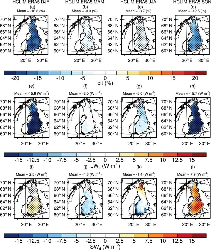
The modeled seasonal averages of total cloud fraction (clt), RoadSurf was driven using an RCM that was forced by a
SWd , LWd , RH, and WS were compared against the ERA5 reanalysis product only in the lateral boundaries. This im-
reanalysis product over 2002–2014 since these parameters, plies that the modeled day-to-day variability might not en-
excluding clt, were used as inputs for RoadSurf together with tirely match with observations at all locations. However, cal-
Tair and precipitation. Again, the stippled areas in Fig. 8 il- culating monthly statistics gives us a clear understanding of
lustrate significant differences revealed by the Student’s t test the model performance for different months during the study
(p < 0.05). Clt was significantly underestimated throughout period from 2002 to 2014.
the year with the highest domain-averaged bias of −16.3 % Figure 9 makes it evident that the HCLIM-driven
in the winter (Fig. 8a–d). Consequently, LWd was signif- RoadSurf was able to simulate the monthly means of Troad
icantly underestimated during the winter, summer (in the with high accuracy and with most of the biases falling be-
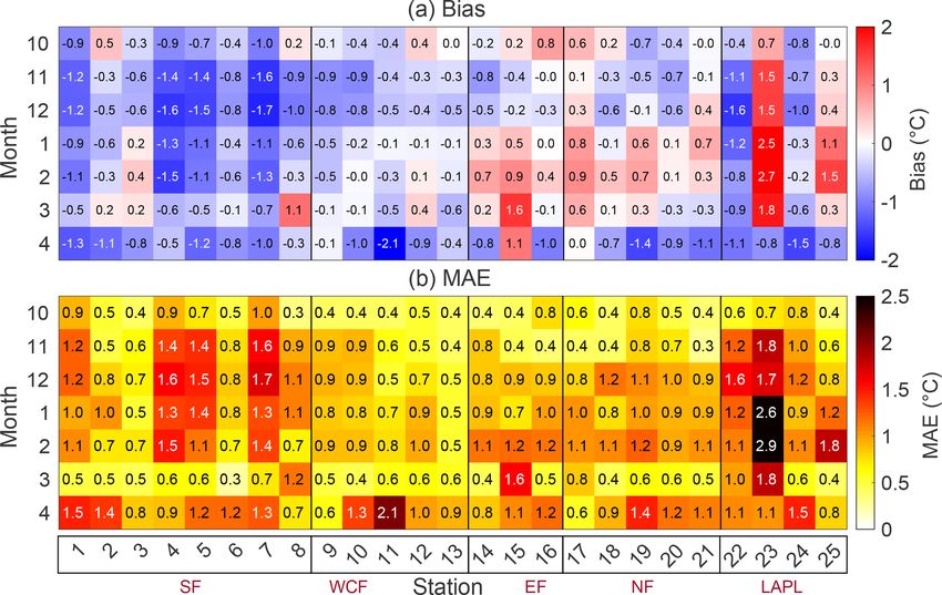
north), and autumn with the largest domain-averaged bias of tween ±2 ◦ C. The mean monthly bias at all 25 stations was
−15.7 W m−2 occurring in the autumn (Fig. 8e–h). SWd was, −0.3 ◦ C (range −2.1 to 2.7 ◦ C) and MAE 0.9 ◦ C (range 0.3–
in turn, mostly significantly overestimated, especially during 2.9 ◦ C). Some regional and seasonal differences were appar-
the autumn when the domain-averaged bias was 7.9 W m−2 ent. In January and February, most of the stations located
(Fig. 8i–l). The biases in SWd during the winter were small in Southern Finland and Western and Central Finland had
as the received actual SWd is, in general, limited during this mainly negative mean biases, whereas the biases were pre-
time of the year at the high latitudes. However, negative bi- dominantly positive at the stations located in Eastern Fin-
ases in SWd were found over the southern parts of Finland land, Northern Finland, and Lapland. When looking at the
during the spring and summer, although the differences were results for all stations, most of the positive mean biases oc-
www.geosci-model-dev.net/12/3481/2019/ Geosci. Model Dev., 12, 3481–3501, 2019
3490                                                           E. Toivonen et al.: The road weather model RoadSurf (v6.60b)

Figure 6. (a–d) The reference values of precipitation (Pr) from E-OBS data and (e–h) the biases of HCLIM38-ALARO modeled Pr with a
reference to E-OBS. The seasonal averages were calculated for the time period of January 2002–December 2014. Stippled areas represent
statistically significant differences with p values < 0.05.

                                                                     with the largest deviations found in the winter (Fig. S4) in
                                                                     accordance with the PDFs of daily Tair .
                                                                        Probable reasons for the seasonal and regional differences
                                                                     in the model performance are the biases in the HCLIM38-
                                                                     ALARO data and the fact that RoadSurf works well in the
                                                                     vicinity of 0 ◦ C. To address the impact of the biases in the in-
                                                                     put parameters on the Troad biases, we computed the monthly
                                                                     mean biases in the HCLIM38-ALARO model outputs with
                                                                     a reference to E-OBS (in the case of Tair and precipitation)
                                                                     and ERA5 (in the case of LWd , SWd , RH, and WS) at the
                                                                     grid cell closest to the road weather station in question. The
                                                                     monthly biases in the input parameters were plotted against
                                                                     the monthly biases in Troad . The analysis shown in Fig. 10
Figure 7. The monthly mean biases of simulated precipitation av-
                                                                     revealed that the variability in the monthly biases of Tair
eraged over Southern Finland (SF), Western and Central Finland
                                                                     explained on average 57 % (range 19 %–84 % in October–
(WCF), Eastern Finland (EF), Northern Finland (NF), Lapland
(LAPL), and the whole of Finland (ALL) in 2002–2014 with a ref-      April) of the variability in the monthly biases of Troad while
erence to E-OBS.                                                     the LWd biases explained on average 16 % (range 2 %–34 %
                                                                     in October–March). Furthermore, the variability in SWd bi-
                                                                     ases was found to explain a small amount (4 %) of the vari-
curred in January and March, whereas negative biases oc-             ability in Troad biases during April. The comparison between
curred in April, November, and December. Eleven stations             other input parameters and Troad did not reveal clear linear
had negative mean biases throughout all the analyzed months          responses and are thus not discussed here. Also, Karsisto et
while the rest of the stations had both negative and positive        al. (2017) noted that a part of the Troad biases is caused by
mean biases depending on the month. Overall, the MAE val-            the biases in the input parameters used to force road weather
ues were the lowest in March and October while the highest           models. In their study, the input was provided by a fore-
MAE values occurred in Lapland in January and February.              cast produced with a high-resolution NWP version of HAR-
Despite the apparent mean monthly biases, the shapes of the          MONIE (cy36h1.4) with a grid resolution of 2.5 km over the
daily Troad PDFs were sufficiently reproduced by RoadSurf            Netherlands. In that study, the KNMI (the Royal Netherlands

Geosci. Model Dev., 12, 3481–3501, 2019                                                www.geosci-model-dev.net/12/3481/2019/
E. Toivonen et al.: The road weather model RoadSurf (v6.60b) 3491 Figure 8. The biases in the simulated seasonal means of (a–d) total cloud fraction (clt), (e–h) downwelling longwave and (i–l) shortwave radiation (LWd and SWd , respectively) with a reference to the ERA5 reanalysis product. The seasonal mean biases were calculated over Finland for the time period of January 2002–December 2014. Stippled areas represent statistically significant differences with p values < 0.05. Meteorological Institute) road weather model (a 1-D heat in the modeled Troad at the northernmost stations. In addi- balance model similar to RoadSurf) was run by removing tion, Kangas et al. (2015) noted that RoadSurf is designed the bias of one of the model inputs, 2 m Tair . This reduced to work especially well when temperatures are close to 0 ◦ C. the Troad bias during the nighttime by 50 % indicating that Based on the monthly statistics obtained for the study pe- the biases in the input parameters clearly affect road weather riod (2002–2014), road surface temperatures were crossing model outcomes. 0 ◦ C particularly often during March, April, and October (see Moreover, the comparison of the simulated and observed Sect. 3.2.2). This good model performance near 0 ◦ C could, Tair in the wintertime (December–February) revealed a warm in turn, partly explain why the MAE values were lower in bias ranging from 0.1 to 1.1 ◦ C in the northern parts of Fin- October and March compared to other months. land (Northern Finland and Lapland) while Southern Finland Some part of the biases in Troad might originate from the had negative biases ranging between −0.4 and −0.04 ◦ C (see RoadSurf model itself. For instance, the absence of snow re- Fig. 4). Thus, the larger and more positive biases in the sim- moval and salting in the model might keep the road surface ulated Tair in Northern Finland and Lapland compared to colder than what it would be with the maintenance actions. Southern Finland seem to explain the larger positive biases In addition, traffic is assumed to pack some part of the snow www.geosci-model-dev.net/12/3481/2019/ Geosci. Model Dev., 12, 3481–3501, 2019
3492                                                              E. Toivonen et al.: The road weather model RoadSurf (v6.60b)

Figure 9. (a) The mean monthly biases and (b) MAE values of simulated road surface temperature between October and April in 2002–2014.
The station indices on the x axis refer to Table 1. SF refers to Southern Finland, WCF to Western and Central Finland, EF to Eastern Finland,
NF to Northern Finland, and LAPL to Lapland.

Figure 10. Scatter plots of the mean monthly biases of road surface temperature (Troad ) against (a) the mean monthly biases of near-surface
air temperature (Tair ) and (b) the mean monthly biases of downwelling longwave (LWd for October–March) and shortwave radiation (SWd
for April) at the road weather stations. The squared R values represent linear regression for different months with p values < 0.001 (p value
for LWd in October 0.01).

into ice while the remaining part is assumed to be blown                 the other hand, the snowpack that is observed might actu-
away from the road. For example, the real traffic amounts                ally stay longer than what is simulated by the model leading
are higher in Southern Finland compared to the other parts               to positive biases in Troad at locations with less traffic: this
of the country, which can lead to an overestimation of the               could especially happen at stations such as station 23 (Siep-
simulated icy and snowy conditions in the south and, hence,              pijärvi). The biases in Troad might also stem from the absence
to colder road surface conditions than what is observed. On

Geosci. Model Dev., 12, 3481–3501, 2019                                                     www.geosci-model-dev.net/12/3481/2019/
E. Toivonen et al.: The road weather model RoadSurf (v6.60b) 3493
of shading effects as this effect is not taken into account by days declined in March and increased in April when mov-
RoadSurf. ing towards the north. In Lapland, most of the zero crossings
Although the results obtained in this study indicated a occurred in April instead of March. This was also expected
good skill of RoadSurf to realistically capture Troad , the mean as the winter season (and therefore the coldest period) lasts
biases were slightly larger compared to the previous studies longer in Lapland compared to the southern parts of Finland,
of RoadSurf. For example, Karsisto et al. (2016) found that leading to less zero-crossing days in March. The smallest
the biases in the simulated Troad varied between −1 and 1 ◦ C number of zero crossings took place in January, February,
(mostly ±2 ◦ C in our study) at 20 stations in Finland during and December. These are usually the coldest months of the
October and December 2013 when RoadSurf was driven by year, especially in Lapland (see also Table 1); thus, 0 ◦ C is
a high-resolution NWP version of HARMONIE (cy36h1.4) not crossed as often during these months.
with a grid resolution of 2.5 km without any data assimila-
tion. However, it is good to note that the results obtained in 3.2.3 Road surface classes
our study and by Karsisto et al. (2016) are not directly com-
parable since in their study RoadSurf was initialized using The majority of the wintertime and weather-related road
road weather station measurements for 48 h and only the first accidents in Fennoscandia are caused by the snowy and
forecasted hour was analyzed. However, one possible reason icy road conditions in addition to, for example, driving
for the slightly larger errors obtained in the present study habits and worn out tires (Salli et al., 2008). To investigate
might be the coarser grid resolution of HCLIM38-ALARO RoadSurf’s skill to correctly predict the road surface classes
as compared to the NWP version: coarser grid resolution im- (e.g. snowy and icy surfaces), the model results and obser-
plies that not all the local features, such as topography, are vations were compared by calculating the fraction of each
described as in detail as they are in higher resolution NWP road surface class occurring within a month. The fraction
models. Increasing the grid resolution of HCLIM38-ALARO was calculated as a multiyear sum of the occurrence of the
might therefore yield better performance for RoadSurf al- surface class in question divided by the multiyear sum of the
though increasing the grid resolution of a climate model will occurrence of all surface classes and then taking an average
also increase the computational cost. However, the longer between stations falling into the same region. It is good to re-
time period used in this study makes the results more robust member that the observed and modeled road surface classes
compared to the previous studies in which only short time might not fully match as they are defined differently.
periods were analyzed. Figure 12 shows that overall RoadSurf captured well the
prevailing road surface conditions although the observed and
3.2.2 Zero-crossing days modeled fractions differed slightly. For example, the model
overestimated the fraction of dry surfaces in all regions (av-
Temperatures close to 0 ◦ C should be predicted correctly be- erage bias over all regions and all months was 7 % as a frac-
cause in these conditions wet road surfaces have a tendency tion) and underestimated damp surfaces slightly more (av-
to freeze (e.g. Vajda et al., 2014) and roads are the most slip- erage bias −16 %). The model underestimated also wet sur-
pery in the copresence of ice (Moore, 1975). In this study, a faces (average bias −6 %), but the fraction of the partly icy
zero-crossing day was defined as a day when the road surface class (8 % on average) was almost equal to this difference be-
temperature had been at least once both below −0.5 ◦ C and tween the modeled and observed wet surface fraction. There-
above 0.5 ◦ C. fore, these results indicated that wet surfaces tended to be
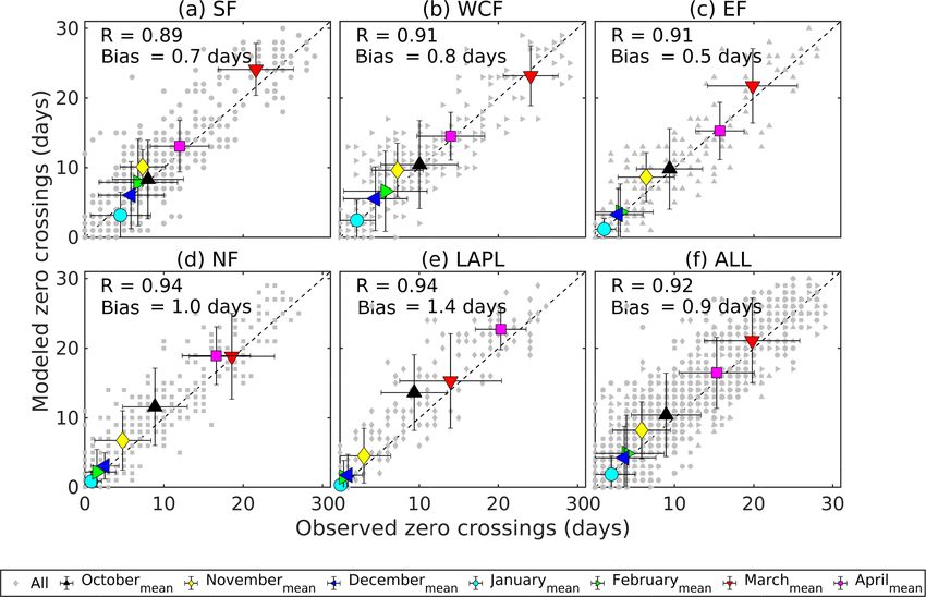
Figure 11 shows that the monthly number of zero-crossing predicted as partly icy, although it has to be remembered that
days and the monthly variation (standard deviation) were observations do not have a partly icy class. The underestima-
well captured by RoadSurf. This was expected as RoadSurf tion of the frost on the road (average bias −1 %) and overes-
has been confirmed to simulate Troad accurately in the vicin- timation of ice (2 %) were also of a similar magnitude with
ity of 0 ◦ C (Kangas et al., 2015; Karsisto et al., 2016). On opposite signs. Moreover, the snow class was slightly overes-
average, the correlation coefficient was very high (0.92) and timated with an average bias of 2 %. These results are in line
the mean bias was approximately 0.9 d (Fig. 11f). The perfor- with the study by Kangas et al. (2015) where they encoun-
mance of the model differed slightly depending on the ana- tered an overestimation of ice and snow storages produced
lyzed region. Surprisingly, the correlation coefficient was the by RoadSurf at two stations located in Finland. In addition,
lowest in Southern Finland and the highest in Northern Fin- they found that sometimes frost predicted by the model was
land and Lapland, whereas the bias was the lowest in Eastern observed as ice in the measurements. In the present study,
Finland and the highest in Lapland. The higher biases in La- frosty surfaces were, however, mainly underestimated. On
pland might be explained by the overall overestimation of the other hand, both icy and frosty surfaces are slippery, so
zero-crossing days, which might, in turn, be caused by the in that aspect the model behavior (i.e., the tendency of the
warm bias in the simulated Troad values as discussed before. model to underestimate frost and to overestimate ice with the
Overall, most of the zero-crossing days occurred in March, same magnitude) is acceptable.
April, and October. However, the number of zero-crossing
www.geosci-model-dev.net/12/3481/2019/ Geosci. Model Dev., 12, 3481–3501, 20193494 E. Toivonen et al.: The road weather model RoadSurf (v6.60b) Figure 11. Modeled vs. observed days per month when road temperatures had been both below −0.5 ◦ C and above 0.5 ◦ C (zero-crossing day) during October and April in 2002–2014 in (a) Southern Finland (SF), (b) Western and Central Finland (WCF), (c) Eastern Finland (EF), (d) Northern Finland (NF), (e) Lapland (LAPL), and (f) the whole of Finland (ALL). Grey color represents the monthly values for every year and the multiyear monthly means are illustrated in other colors. The vertical and horizontal bars represent ±1 standard deviation based on 13 years of monthly values from the model and observations, respectively. R stands for the Pearson correlation coefficient and BIAS for the mean difference between the modeled and observed values. The dashed black line represents a 1 : 1 reference line. Figure 12. Observed (O) and modeled (M) fractions of road surface classes (e.g. dry, wet, or icy) within each month in 2002–2014 in (a) Southern Finland (SF), (b) Western and Central Finland (WCF), (c) Eastern Finland (EF), (d) Northern Finland (NF), (e) Lapland (LAPL), and (f) the averages for whole of Finland (ALL). The definitions of road surface classes differ slightly for the observations and model (e.g. the partly icy class is included only in the model). The absence of road maintenance could be one logical rea- ing, is performed far less frequently compared to the more son why the model overestimated icy and snowy surfaces: in southern parts of Finland in real life. The icy road fraction real life, salting prevents roads becoming icy and snow is re- was underestimated in Lapland, whereas this fraction was moved from the roads. Accordingly, the observed and mod- overestimated in the other regions: in reality, salting is not eled fractions of snowy surfaces were very similar to each performed as often at the stations in Lapland as in South- other in Lapland where maintenance, such as snow plow- ern Finland and thus icy roads can occur more frequently in Geosci. Model Dev., 12, 3481–3501, 2019 www.geosci-model-dev.net/12/3481/2019/
You can also read