Spatial and temporal variability of snowfall over Greenland from CloudSat observations - Atmos. Chem. Phys
←
→
Page content transcription
If your browser does not render page correctly, please read the page content below
Atmos. Chem. Phys., 19, 8101–8121, 2019
https://doi.org/10.5194/acp-19-8101-2019
© Author(s) 2019. This work is distributed under
the Creative Commons Attribution 4.0 License.

Spatial and temporal variability of snowfall over Greenland
from CloudSat observations
Ralf Bennartz1,2 , Frank Fell3 , Claire Pettersen2 , Matthew D. Shupe4 , and Dirk Schuettemeyer5
1 Earth and Environmental Sciences Department, Vanderbilt University, Nashville, Tennessee, USA
2 Space  Science and Engineering Center, University of Wisconsin – Madison, Madison, Wisconsin, USA
3 Informus GmbH, Berlin, Germany
4 Physical Sciences Division, Cooperative Institute for Research in Environmental Science and

NOAA Earth System Research Laboratory, Boulder, Colorado, USA
5 ESA ESTEC, Noordwijk, the Netherlands

Correspondence: Ralf Bennartz (ralf.bennartz@vanderbilt.edu)

Received: 30 September 2018 – Discussion started: 7 January 2019
Revised: 15 April 2019 – Accepted: 22 May 2019 – Published: 21 June 2019

Abstract. We use the CloudSat 2006–2016 data record to            ferred from CloudSat to be 34 ± 7.5 cm yr−1 liquid equiva-
estimate snowfall over the Greenland Ice Sheet (GrIS). We         lent (where the uncertainty is determined by the range in val-
first evaluate CloudSat snowfall retrievals with respect to re-   ues between the three different Z–S relationships used). In
maining ground-clutter issues. Comparing CloudSat obser-          comparison, the ERA-Interim reanalysis product only yields
vations to the GrIS topography (obtained from airborne al-        30 cm yr−1 liquid equivalent snowfall, where the majority of
timetry measurements during IceBridge) we find that at the        the underestimation in the reanalysis appears to occur in the
edges of the GrIS spurious high-snowfall retrievals caused        summer months over the higher GrIS and appears to be re-
by ground clutter occasionally affect the operational snow-       lated to shallow precipitation events. Comparing all available
fall product. After correcting for this effect, the height of     estimates of snowfall accumulation at Summit Station, we
the lowest valid CloudSat observation is about 1200 m above       find the annually averaged liquid equivalent snowfall from
the local topography as defined by IceBridge. We then use         the stake field to be between 20 and 24 cm yr−1 , depend-
ground-based millimeter wavelength cloud radar (MMCR)             ing on the assumed snowpack density and from CloudSat
observations obtained from the Integrated Characterization        23 ± 4.5 cm yr−1 . The annual cycle at Summit is generally
of Energy, Clouds, Atmospheric state, and Precipitation at        similar between all data sources, with the exception of ERA-
Summit, Greenland (ICECAPS) experiment to devise a sim-           Interim reanalysis, which shows the aforementioned under-
ple, empirical correction to account for precipitation pro-       estimation during summer months.
cesses occurring between the height of the observed Cloud-
Sat reflectivities and the snowfall near the surface. Using the
height-corrected, clutter-cleared CloudSat reflectivities we
next evaluate various Z–S relationships in terms of snowfall      1   Introduction
accumulation at Summit through comparison with weekly
stake field observations of snow accumulation available since     The Greenland Ice Sheet (GrIS) is currently losing mass at a
2007. Using a set of three Z–S relationships that best agree      rate of roughly 240 Gt yr−1 , translating into a sea level rise
with the observed accumulation at Summit, we then calcu-          of 0.47 ± 0.23 mm yr−1 (van den Broeke et al., 2016), which
late the annual cycle snowfall over the entire GrIS as well as    corresponds to roughly 15 %–20 % of the total annual mean
over different drainage areas and compare the derived mean        sea level rise. Precipitation is the sole source of mass of the
values and annual cycles of snowfall to ERA-Interim reanal-       GrIS. Additionally, the inter-annual precipitation variability
ysis. We find the annual mean snowfall over the GrIS in-          appears to be the main driver of inter-annual variability in
                                                                  the mass balance of the GrIS (van den Broeke et al., 2009).

Published by Copernicus Publications on behalf of the European Geosciences Union.
8102                                        R. Bennartz et al.: Spatial and temporal variability of snowfall over Greenland

It is also the largest source of uncertainty in the surface mass   plied to CloudSat. Based on these corrections and findings,
balance of the GrIS (van den Broeke et al., 2009). At the          we then calculate our best estimates of surface snowfall from
same time, ground-based long-term observations of precip-          all available CloudSat observations and assess the annual cy-
itation over the GrIS are sparse. Over the GrIS surface sta-       cle and spatial distribution of snowfall over the entire GrIS.
tion networks include the Greenland Climate Network (GC-              The remainder of this paper is structured as follows:
NET; Box and Steffen, 2000) and the Programme for Moni-            in Sect. 2 we discuss the different data source including
toring of the Greenland Ice Sheet (PROMICE; by the Danish          the ground-based observations at Summit Station, CloudSat
Energy Agency; van As, 2017). These networks of surface            satellite observations, and reanalysis products. Section 3 ad-
stations do not directly observe precipitation; however lim-       dresses the aforementioned issues related to using CloudSat
ited information on accumulation may be inferred by boom           as a proxy for surface snowfall. In Sect. 4 we compare Cloud-
height measurements using sonic ranging. Van den Broeke            Sat and ERA-Interim reanalysis data products and provide
et al. (2016) point out the importance of individual mass          estimates for the annual cycle of snowfall over the different
sources, i.e., snowfall, contributing to the GrIS surface mass     drainage systems of the GrIS as well as over Summit. Con-
balance which “[...] must be interpolated from scarce in situ      clusions and an outlook are provided in Sect. 5.
measurements and/or simulated using dedicated regional cli-
mate models, which introduces potentially large uncertain-
ties”. Comparison studies of different climate and reanalysis      2     Datasets and methods
models show an about 25 %–40 % spread in snowfall esti-
mates over the GrIS between the different models (Cullather        2.1    CloudSat data
et al., 2014; Vernon et al., 2013).
                                                                   CloudSat (Stephens et al., 2002, 2008) carries the single-
    Since 2006, CloudSat observations have been used in a se-
                                                                   frequency, W-band (94 GHz) cloud-profiling radar (CPR;
ries of studies addressing snowfall globally (Liu, 2008; Hiley
                                                                   Tanelli et al., 2008). The CPR has provided global cloud
et al., 2011; Palerme et al., 2014; Kulie et al., 2016; Adhikari
                                                                   and precipitation profiles since 2006; however, only day-
et al., 2018; Kulie and Milani, 2018). While some of the
                                                                   time scenes can be observed since 2011 due to a hard-
global studies include Greenland, a detailed assessment of
                                                                   ware failure1 . The CPR is a non-scanning, near-nadir point-
snowfall over the GrIS using CloudSat has to our knowledge
                                                                   ing instrument with a mean spatial resolution of ∼ 1.5 km
not yet been performed. Here we present such an assessment.
                                                                   and a vertical range gate spacing of 500 m, although instru-
    Several factors complicate snowfall estimates from Cloud-
                                                                   ment oversampling enables 240 m data bins in the Cloud-
Sat over the GrIS. First, the height of the central GrIS makes
                                                                   Sat data products. In the framework of this study, we use
for a unique environment in terms of snowfall characteristics.
                                                                   the 2C-SNOW-PROFILE (Wood et al., 2014) together with
For example, Pettersen et al. (2018) find that a large frac-
                                                                   the GEOPROF reflectivity profiles and ECMWF-AUX tem-
tion of the total accumulation at Summit Station falls from
                                                                   perature and moisture profiles (Stephens et al., 2008). Prod-
clouds that contain no liquid water with only ice microphys-
                                                                   uct documentation can be obtained from the CloudSat Data
ical processes involved. Secondly, the steep altitude changes
                                                                   Processing Center (DPC, http://www.cloudsat.cira.colostate.
at the edges of the ice sheet pose challenges to the space-
                                                                   edu/, last access: 9 June 2019). All analysis is based on the
borne radar observations due to ground clutter. This issue has
                                                                   CloudSat Release 5 data, which were made publicly available
a compounding impact on CloudSat’s clutter-affected blind
                                                                   by the DPC in June 2018.
zone near the surface, which typically extends from the sur-
                                                                      Figure 1 shows the number of CloudSat measurements
face to about 1200 m (Maahn et al., 2014). Thus, “surface”
                                                                   available over Greenland (top) and within a 50 km range from
snowfall rates observed from CloudSat are typically taken at
                                                                   Summit Station (bottom). One can clearly identify the re-
an altitude of 1200 m above the surface.
                                                                   duction in data coverage after the CloudSat battery failure
    To account for the above issues related to surface topog-
                                                                   in April 2011. Even after operations were restored, data col-
raphy and CloudSat’s blind zone, we use auxiliary informa-
                                                                   lection was limited to the sunlit part of the orbit, leading to
tion about the GrIS surface topography (the IceBridge Bed-
                                                                   an annual cycle in the number of observations available over
Machine V3 topography; Morlighem et al., 2017) to better
                                                                   Greenland.
characterize which CloudSat radar bin can be regarded as the
                                                                      Figure 2 shows the spatial distribution of these mea-
lowest clutter-free observation. We then use millimeter wave-
                                                                   surements over Greenland. Because of CloudSat’s 16 d re-
length cloud radar (MMCR) observations from ICECAPS
                                                                   peat pattern, coverage at high spatial resolution creates a
to estimate the impact of CloudSat’s observation height on
                                                                   diamond-shaped pattern over Greenland, as can be seen in
estimated surface snowfall, and we propose a simple GrIS-
                                                                   Fig. 2b. This pattern limits the maximum resolution of any
specific empirical correction to account for the difference be-
                                                                   climatology based on CloudSat data. For a resolution of
tween actual surface snowfall and the CloudSat observations
made at about 1200 m height above the surface. We further             1 For a detailed timeline of CloudSat availability, see the op-
use ground-based snowfall accumulation from Summit Sta-            erational CloudSat Radar Status blog at https://cloudsat.atmos.
tion to assess the validity of different Z–S relationships ap-     colostate.edu/news/CloudSat_status (last access: 9 June 2019).

Atmos. Chem. Phys., 19, 8101–8121, 2019                                              www.atmos-chem-phys.net/19/8101/2019/
R. Bennartz et al.: Spatial and temporal variability of snowfall over Greenland                                                 8103

Figure 1. Number of CloudSat observations per month all over Greenland (a) and within 50 km of Summit Station (b).

Figure 2. CloudSat data density over Greenland at 1◦ × 2◦ (a, corresponding to 100 km × 100 km at 60◦ N) and 0.025◦ × 0.05◦ (b, corre-
sponding to 2.5 km × 2.5 km at 60◦ N). Shown is the total number of observations per grid box over the time period from 2006 to 2016.

roughly 100 km × 100 km, the coverage appears fairly uni-            tion at Summit Station, located near the apex of the GrIS at
form apart from a north–south gradient, which is a result            an elevation of 3200 m above sea level (Shupe et al., 2013).
of the better coverage near the maximum coverage latitude            These instruments have been in operation at the NSF Mobile
around 81.8◦ , due to CloudSat’s inclination of about 98.2◦ .        Science Facility nearly continuously since July 2010. This
                                                                     comprehensive dataset of atmospheric properties above the
2.2   ICECAPS observations                                           GrIS is unprecedented, due to both the large number of dis-
                                                                     tinct and complementary measurements that are being made
The ICECAPS (Integrated Characterization of Energy,                  and the length of the time series.
Clouds, Atmospheric state, and Precipitation at Summit) ex-             The ICECAPS experiment, as well as instrument specifi-
periment operates a sophisticated suite of instruments that          cations, measurements, and derived products, are described
observe properties of the atmosphere, clouds, and precipita-

www.atmos-chem-phys.net/19/8101/2019/                                                  Atmos. Chem. Phys., 19, 8101–8121, 2019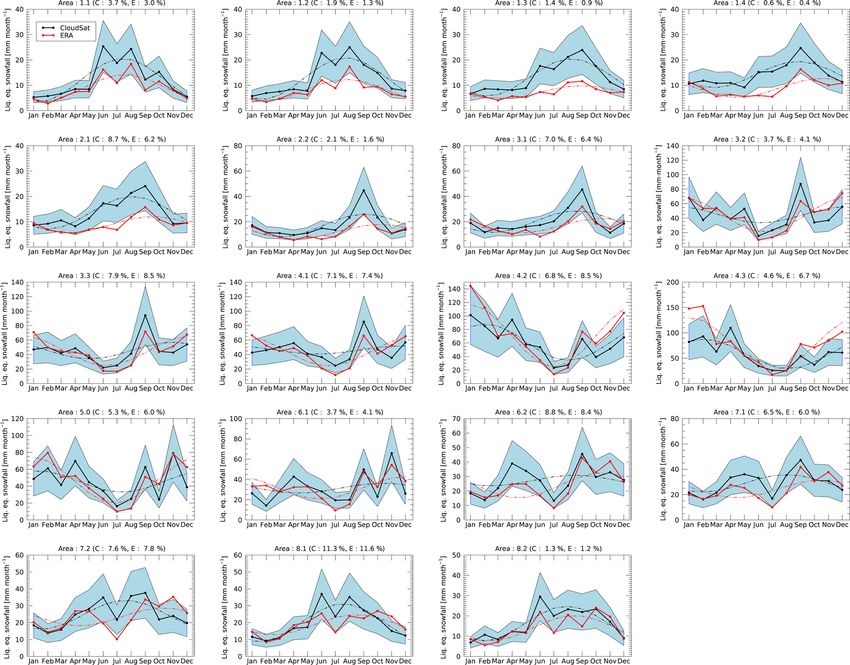
8104                                       R. Bennartz et al.: Spatial and temporal variability of snowfall over Greenland

in Shupe et al. (2013). In particular, the Ka-band MMCR,          2.4   Z–S relations used in this study
the X-band Precipitation Occurrence Sensor System (POSS),
and the Multi-Angle Snowflake Camera (MASC, 2015–                 To compare CloudSat CPR and the MMCR, we apply a set
2016, selected dates only) are of relevance with respect          of different published Z–S relationships as well as Z–S rela-
to precipitation. In this study we build on earlier work by       tionships empirically fitted to some of the observational data.
Castellani et al. (2015) and Pettersen et al. (2018). The lat-    The Z–S relationships used are summarized in Table 1. In
ter study also provides a combined dataset of relevant pa-        addition to the Matrosov (2007, hereafter M07) relationship
rameters for studying precipitation variability over the cen-     used in various previous studies, we employ a set of Z–S re-
tral GrIS. This dataset is available with a temporal resolu-      lationships that apply to single habits, which, based on the
tion of 1 min and is used as a basis for the investigations       above considerations and observations, might be better prox-
performed here but complemented with additional MMCR              ies for snowfall at Summit than M07. While some Z–S rela-
observations. For more details on the MMCR and its calibra-       tionships are only available at Ka band (i.e., MMCR), others
tion, see Castellani et al. (2015) and references therein.        are available only at W band (i.e., CloudSat). Only four Z–
   In addition to these ICECAPS data, other observations are      S relationships are available consistently for both Ka and W
available at Summit Station. Most important in this context       band and, therefore, allow transferring results between the
is the so-called “snow stake field”, which consists of 11 × 11    two bands. Uncertainties of instantaneous snowfall retrievals
bamboo stakes planted in a square a few hundred meters            using Z–S relationships can be large and are discussed in
away from the station. The height of all 121 stakes above the     detail in the publications referenced in the last column of Ta-
snow surface is read off approximately every week, thereby        ble 1. The individual uncertainties should not be confused
creating a unique reference for surface height changes. Once      with systematic errors introduced by the choice of particu-
a year, the stakes are raised by about 70 cm in order to al-      lar Z–S relationships. Such systematic errors are of greater
low for continuous measurements. The stake measurements           importance when generating climatological precipitation es-
go back to 2003, with easily accessible data going back to        timates (as random uncertainties average out in the process
2007, covering the full ICECAPS period, and providing an          of generating, e.g., monthly means). Here we follow an ap-
independent set of observations of snowfall accumulation.         proach developed in our earlier publications (Kulie and Ben-
Similar to Castellani et al. (2015), who provide a discussion     nartz, 2009; Hiley et al., 2011), where we define uncertain-
on the accuracy of the stake field data, we herein use these      ties on the climatological end product in terms of differences
stake observations to assess the other accumulation measure-      between different Z–S relationships. We believe that this ap-
ments, namely from the ground-based and space-borne radar.        proach provides more realistic error estimates on climatolog-
Castellani et al. (2015) address the importance of blowing        ical products (for more details, see Hiley et al., 2011).
snow as a source of noise for individual stake field obser-
vations and suggest using the average of all 121 individual       2.5   Assumption on snowpack density used in this study
stakes as an estimate or the actual accumulation. We follow
their approach. They further discuss existing literature on the   Dibb and Fahnestock (2004), based on snow pits, find
importance of blowing snow over the GrIS and indicate that        snow densities over central Greenland between 240 and
the net effect of blowing snow is small (see Cullen et al.,       370 kg m−3 at depths between 15 and 45 cm, which is prob-
2014).                                                            ably a realistic average depth range for annual accumula-
                                                                  tion studies. More recent results by Fausto et al. (2018)
2.3    ERA-Interim                                                indicate an average density of the uppermost snow layer
                                                                  over Greenland to be 315 ± 44 kg m−3 for the uppermost
ERA-Interim (Dee et al., 2011) is a third-generation global       10 cm and 341 ± 37 kg m−3 for the uppermost 50 cm. Fausto
atmospheric reanalysis provided by the European Centre for        et al. (2018), as well as earlier studies (e.g., Reeh et al.,
Medium-Range Weather Forecasts (ECMWF). It expands on             2005), also find a weak dependency of density on temper-
previous versions (e.g., ERA-40) by using an improved at-         atures. Here we use snowpack density in two ways: firstly,
mospheric model and assimilation system (ECMWF, 4D-               in Sect. 3.4.2 we use the stake field observations as a refer-
VAR, 2006). The spatial resolution of the dataset is approx-      ence to assess the validity of different CloudSat-based Z–S
imately 80 km (T255 spectral) on 60 vertical levels from          relationships. Following the work of Castellani et al. (2015),
the surface up to 0.1 hPa. Among other data, it assimi-           we compared the stake field data with CloudSat-based liquid
lates data from a number of satellites. ERA-Interim data          equivalent snowfall rates by calculating the effective density
are available since 1979 and are continuously updated. For        needed for the CloudSat snowfall estimates to match the ob-
this study, monthly gridded snowfall estimates were used          served accumulation. We then reject as unrealistic Z–S rela-
(downloaded from https://rda.ucar.edu/datasets/ds627.0/, last     tionships that fall outside the above wide range of densities
access: 9 June 2019).                                             reported for Summit. Secondly, in Sect. 4.2 we compare the
                                                                  annual cycle of liquid equivalent snowfall over Summit from
                                                                  different observations. To convert the stake field values into

Atmos. Chem. Phys., 19, 8101–8121, 2019                                            www.atmos-chem-phys.net/19/8101/2019/
R. Bennartz et al.: Spatial and temporal variability of snowfall over Greenland                                                      8105

Table 1. Parameters of Ka-band (MMCR) Z–S relations and W band (CloudSat) used in this study. The POSS operates at X band so that the
Z–S relation is not directly comparable to the Z–S relations for MMCR. A Z–S relationship is defined as Z = AS B where S is the snowfall
rate (in mm h−1 ) and Z the radar reflectivity (in mm6 m−3 ).

        Name          A (Ka band)    B (Ka band)     A (W band)     B (W band)    Reference
        M07                  56.0            1.20           10.0           0.80   Castellani et al. (2015), Matrosov (2007),
                                                                                  Pettersen et al. (2018)
        KB09_LR3             24.0            1.51           13.2           1.40   Kulie and Bennartz (2009), using Liu (2008)
                                                                                  three-bullet rosettes
        KB09_HA             313.3            1.85           56.4           1.52   Kulie and Bennartz (2009), using Hong (2007)
                                                                                  aggregates
        L08                      –               –          11.5           1.25   Liu (2008)
        HI11_L                   –               –           7.6           1.30   Hiley et al. (2011)
        HI11_A                   –               –          21.6           1.20   Hiley et al. (2011)
        HI11_H                   –               –          61.2           1.10   Hiley et al. (2011)
        POSS                   n/a             n/a             –              –   Pettersen et al. (2018), Sheppard and Joe (2008)

liquid equivalent snowfall we use the conversions proposed            radar reflectivity itself, as well as from an underlying digital
by Fausto et al. (2018) and Reeh et al. (2005) to provide a           elevation model.
range of liquid equivalent snowfall rates based on the stake             In our analysis, we found that the height of the surface bin
field observations.                                                   is not always accurately represented over Greenland. This oc-
                                                                      casionally causes significant outliers in the retrieved surface
                                                                      snowfall rate. In order to study and possibly correct for this
3     Evaluation of CloudSat observations                             issue, we use the IceBridge BedMachine (V3) surface topog-
                                                                      raphy measurements (Morlighem et al., 2017) and collocate
Here we assess the full CloudSat snowfall dataset over                those with each individual CloudSat observation. We then
Greenland in terms of its viability for climatological snow-          re-derive the snowfall rates based on the fifth radar bin above
fall studies. Amount and spatial distribution of the data used        the surface as defined by this new topography. We compare
for this assessment are shown in Figs. 1 and 2. We analyze            these new retrievals to the originally retrieved snowfall rates,
the dataset with respect to the following issues:                     which also typically are taken from the fifth radar bin above
    a Effects and removal of ground clutter.                          the surface, but with a different prescribed surface eleva-
                                                                      tion model defining the surface. We restrict our analysis to
    b. Impact of height of CloudSat observation above the sur-        SNOWPROF confidence flag values 3 and 4, which indicate
       face.                                                          high confidence in the retrieval.
                                                                         The difference in elevation reported between CloudSat and
    c. Impact of choice of Z–S relationship.                          BedMachine can be seen in Fig. 3. It is not entirely unrealis-
                                                                      tic that some of the differences seen between the two digital
At Summit, concurrent observations from the snow stake                elevation models may be caused by melting in the ablation
field and MMCR allow for a detailed assessment of these               zone. However, differences might also be caused by other
issues.                                                               factors. Clearly, some of the coastal regions with the largest
                                                                      differences experience significant amounts of snowfall. The
3.1    Effects and removal of ground clutter
                                                                      impact of using different underlying surface topographies
CloudSat observations in the lowest range bins above the sur-         for snowfall retrieval and accumulation is shown in Figs. 4
face are affected by ground clutter. Because of topography,           through 6.
this effect is more pronounced over land than over ocean.                Figure 4 shows two-dimensional histograms of radar re-
The CloudSat SNOWPROF product accounts for the impact                 flectivity and derived SNOWPROF surface snowfall rate. For
of ground clutter by providing a confidence flag for the re-          each reported snowfall rate, the corresponding radar reflec-
trieved surface snowfall rates. This flag depends on the type         tivity was obtained from the CloudSat GEOPROF product.
of surface as well as on other criteria, such as vertical consis-     Figure 4a shows the surface snowfall rate and reflectivity
tency of retrieved snowfall rates. A key input over the highly        reported directly from the product. Figure 4b shows the re-
structured coastal terrain of Greenland and the edges of the          vised snowfall rate accounting for the BedMachine topogra-
GrIS is the height of the surface bin, which describes where          phy. Note that for Fig. 4b all snowfall rates are also directly
the radar beam first interacts with the surface. This quantity        retrieved from SNOWPROF. In contrast to Fig. 4a, the snow-
is provided in the CloudSat data and is retrieved from the            fall rates are occasionally taken from radar bins higher in the

www.atmos-chem-phys.net/19/8101/2019/                                                   Atmos. Chem. Phys., 19, 8101–8121, 2019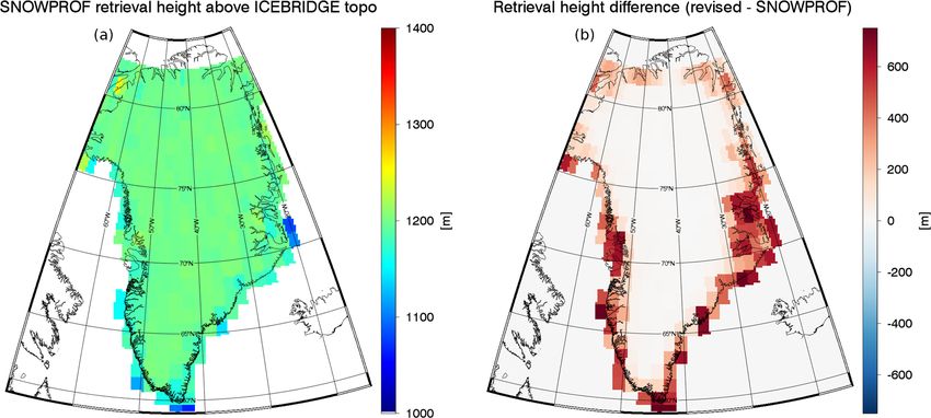
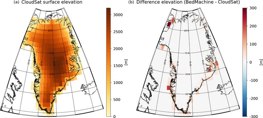
8106                                          R. Bennartz et al.: Spatial and temporal variability of snowfall over Greenland

Figure 3. Panel (a) shows the mean elevation reported from CloudSat binned to 1◦ × 2◦ . Panel (b) shows the difference between the elevation
difference between IceBridge BedMachine v3 (Morlighem et al., 2017) and CloudSat. Note that open water and sea ice observations are
excluded from the dataset, so that differences observed near the coast only stem from ice-free land or GrIS observations within each grid
box.

Figure 4. Histogram of occurrence of snowfall rate versus radar reflectivity for the entire CloudSat dataset over Greenland. Panel (a) shows
the relation if the SNOWPROF surface snowfall rate is used as provided in the original SNOWPROF product. Panel (b) shows the relation
with corrected topography. Different Z–S relations are shown as well.

atmosphere to account for the higher topography estimates               between the original SNOWPROF heights and the revised
from BedMachine.                                                        heights. It can be seen that in the original formulation the
   Comparing the panels in Fig. 4, we note that there is a              distance to the surface near the coast is often in the 1000 m
significant number of high reflectivities associated with very          range, which would likely lead to ground clutter (Maahn et
high and often physically implausible snowfall rates of up to           al., 2014), in particular given the complex orography. Note
50 mm h−1 (see upper right part of Fig. 4a). Using the Bed-             that Fig. 5 shows the effect of the correction on the height
Machine topography to update the estimated surface elimi-               of the lowest valid CloudSat observation above the surface
nates these high snowfall rates (see Fig. 4b). A visual inspec-         (whereas Fig. 3 only shows the difference between two to-
tion of a few of these cases indicates these are clutter-affected       pographies). The impact of these differences in topographies
observations in the original CloudSat product, which are suc-           (see Fig. 3) is amplified as CloudSat observations are binned
cessfully eliminated using the BedMachine topography. The               at 240 m vertical resolution. Because of this 240 m binning,
revised formulation for the lowest valid CloudSat bin above             the slight changes in height observed in Fig. 3 can result in
the surface thus leads to a significant reduction of surface            larger changes in CloudSat observation height as indicated in
clutter as shown in Fig. 4.                                             Fig. 5 (e.g., a difference in topography of 50 m might lead to
   The impact of the above revisions can be seen in Fig. 5,             the lowest valid CloudSat bin increasing by 240 m).
which shows the actual heights of CloudSat surface snowfall                Over the central GrIS the average observation height is
rate observations above the surface, as well as the difference          not affected. We have examined this for the 1◦ × 2◦ grid

Atmos. Chem. Phys., 19, 8101–8121, 2019                                                    www.atmos-chem-phys.net/19/8101/2019/
R. Bennartz et al.: Spatial and temporal variability of snowfall over Greenland                                                    8107

Figure 5. Panel (a) shows the height of the CloudSat SNOWPROF surface snowfall rate observation above the local topography (from
IceBridge BedMachine). Panel (b) shows the difference between the height used in the revised product and original height. For example, at
the southern tip of Greenland, the surface snowfall rate reported in the SNOWPROF product comes from an actual altitude of about 1000 m
above the surface. In the revised formulation discussed in the text, this height is pushed up by 500 to 1500 m.

box around Summit Station, where typically the fifth radar
bin above the surface is selected (around 1200 m above the
surface). In general, it is important to bear in mind that the
CloudSat surface snowfall rate observations over structured
terrain typically come from about 1200 m above the sur-
face and thus do not observe precipitation processes below
that altitude. The impact of CloudSat’s “blind zone”, where
measurements are affected by ground clutter, below roughly
1200 m above ground for the high GrIS is studied in Sect. 3.2.
   Figure 6 shows the integrated effect of the ground-clutter
artifacts in the CloudSat surface snowfall rates on accumu-
lation. The mean snowfall rate for all CloudSat data over
Greenland would be approximately 0.225 mm h−1 in the re-               Figure 6. Impact of surface topography issues on cumulative snow-
vised formulation. Not correcting for artifacts reduces the            fall rates.
mean by 15 % to about 0.2 mm h−1 , but with significant con-
tributions from reflectivities larger than 20 dBZ, which are
eliminated when the IceBridge BedMachine surface topog-                fall rates we use here are also available in the SNOWPROF
raphy is applied. Observations that are corrected for ground           product. However, occasionally, mostly near the coasts, our
clutter contribute toward the total snowfall at lower reflec-          analysis uses snowfall data from higher radar bins than the
tivities, thereby increasing retrieved snowfall rates between          SNOWPROF surface snowfall rates to avoid clutter artifacts
+5 and +15 dBZ and increasing snowfall rate in this dBZ                that would otherwise be present. We note that, while our
interval. Note that Fig. 6 only presents the grand mean of all         paper was under review as a discussion paper, the issue of
snowfall rates. Because of the large differences in surface el-        ground clutter was also studied independently by Palerme et
evation between CloudSat and BedMachine near the coasts,               al. (2019). Their findings corroborate the results we present
the impact of artifacts in coastal areas will be much higher           here.
when snowfall climatologies are reported. In contrast, these
artifacts will not play a major role in the higher elevations of       3.2   Impact of height of observations above ground on
the GrIS.                                                                    estimated surface snowfall rate
   Based on the results reported in the current section, we
                                                                       As shown in Fig. 5, CloudSat snowfall observations over
will hereafter only use the revised snowfall rates that are
                                                                       Greenland stem from altitudes of around 1200 m above the
obtained using the IceBridge BedMachine surface elevation
                                                                       surface to avoid ground clutter issues. This might cause sev-
and discard the surface snowfall rates reported in the SNOW-
                                                                       eral issues because any precipitation processes happening
PROF product. We again note that the revised surface snow-
                                                                       at lower altitudes are not observed and, consequently, not

www.atmos-chem-phys.net/19/8101/2019/                                                    Atmos. Chem. Phys., 19, 8101–8121, 2019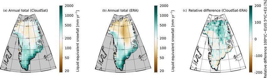
8108                                           R. Bennartz et al.: Spatial and temporal variability of snowfall over Greenland

Figure 7. Panels (a) and (b) show histograms of MMCR observations at Summit. Panel (a) compares radar reflectivity at 135 m above
the surface with the average radar reflectivity between 1000 and 1500 m above the surface, which corresponds to the height range where
CloudSat observations are obtained. Panel (b) shows a similar plot but with a height correction applied. See text for details. Panel (c) shows
cumulative mean snowfall rates for the different radar reflectivities show in (a) and (b).

accounted for in CloudSat estimates. Here we use MMCR
observations from Summit to study the difference between
the observed reflectivities at an altitude of 1200 m and those           dBZcorrected =
closer to the surface (135 m). We first average the vertical                dBZ1000...1500 + [(1 − 0.2 × dBZ1000...1500 ) > 0] .          (1)
reflectivity profile of the MMCR between 1000 and 1500 m
to account for the vertical resolution of CloudSat. After con-           This statistical correction produces the joint histogram
verting the averaged reflectivity back into units of decibel             shown in Fig. 7b and, by design, matches the total cumula-
relative to Z (dBZ), we compare it with the MMCR reflec-                 tive snowfall near the surface (see blue curve in Fig. 7c). The
tivity observed at 135 m above the surface. This compari-                correction was developed by fitting a regression line to the
son is shown in Fig. 7a. One can see that for most cases,                data between −20 and +5 dBZ. The correction drops to zero
the MMCR reflectivity observed at CloudSat height (1000–                 at 5 dBZ and thus does not affect reflectivities higher than
1500 m) is lower than the reflectivity near the surface, pos-            5 dBZ. While the above formula provides larger corrections
sibly owed to precipitation processes occurring at altitudes             to the very low reflectivity values, those corrections affect
below 1000 m. There are also cases where the upper reflec-               snowfall accumulation only very weakly. For example, for
tivity is higher than the reflectivity near the surface. Cases for       an observed reflectivity of −30 dBZ, the correction is +7 dB,
such events could include non-precipitating clouds around                leading to a corrected reflectivity of −23 dBZ, which does
1200 m or ice particles sublimating before they reach the sur-           not produce any significant snowfall.
face (virga). These cases might also include situations where               There are caveats to this correction: importantly, it will
the lowest MMCR radar bin saturates under high reflectivi-               only work if the observed atmospheric states are statistically
ties (see Castellani et al., 2015). Our analysis of this satura-         similar to the ones on which the correction was derived.
tion effect shows that 0.3 % of the MMCR observations are                Since the data used for the correction stems from Summit,
impacted, with only a vanishing effect on the MMCR snow-                 we expect this correction not to produce viable results out-
fall rates reported here. The correction developed in the fol-           side the high elevations of the GrIS. In order to highlight this
lowing paragraph is also not affected. We therefore ignore               limitation, we show in Fig. 8 the same analysis but for Bar-
this saturation effect.                                                  row, Alaska. As one can see, the application of the correction
   By applying the KB09_LR3 Z–S relationship (see Ta-                    outlined in Eq. (1) has no effect on the snowfall rate. This is
ble 1), the red and black curves in Fig. 7c show the impact              because at Barrow snowfall is produced under different at-
of the differences in reflectivity on total cumulative snow-             mospheric conditions. The application of the correction also
fall at Summit. The lower reflectivity at 1000–1500 m yields             does not deteriorate the results at Barrow because it has, by
an underestimation of snowfall rate of about 20 % compared               design, little to no effect on higher reflectivities. This point is
to using the reflectivity near the surface. Most of this differ-         important as near the GrIS ablation zone and in Greenland’s
ence accumulated in a reflectivity range between −10 and                 coastal regions one may expect atmospheric conditions to be
+5 dBZ.                                                                  more similar to Barrow than to Summit.
   In order to correct for this effect, we applied an ad hoc                Results presented in Figs. 7 and 8 apply to the MMCR,
correction that statistically accounts for this effect:                  which operates at Ka band. However, we wish to apply this
                                                                         relationship to CloudSat, which is a W-band radar. Z–S rela-
                                                                         tionships between Ka band and W band are different, because

Atmos. Chem. Phys., 19, 8101–8121, 2019                                                     www.atmos-chem-phys.net/19/8101/2019/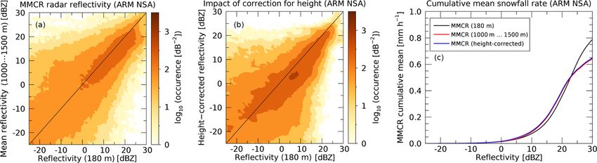
R. Bennartz et al.: Spatial and temporal variability of snowfall over Greenland                                                   8109

Figure 8. Same as Fig. 7 but for the DOE ARM site at the North Slope of Alaska (NSA) at Barrow, Alaska. The figures are based on
1.08 million radar profiles obtained between November 2008 and April 2011. Only data for the winter months of November through April
are shown. The Barrow MMCR data were obtained from https://www.archive.arm.gov/discovery/ (last access: 9 June 2019).

medium-sized ice particles enter the Mie-scattering region at
a smaller size at W band than at Ka band. As snowfall rate
increases, the difference between W band and Ka band typi-
cally increases because the number of large particles outside
the Rayleigh scattering region will increase at W band. This
leads to a different slope of the Z–S relationships at W band
and Ka band, which might affect the correction proposed
here. The Z–S relationships for the two bands are shown in
Fig. 9 for KB09_ LR3. For other Z–S relationships, depend-
ing on the ice particles used and, in particular, the underly-
ing size distribution, these differences can be much larger.
However, as discussed below, KB09_LR3 is likely more rep-
resentative of the light snowfall observed over the high GrIS       Figure 9. Radar reflectivity at Ka band (MMCR) and W band
than other Z–S relationships, which apply more to the mid-          (CloudSat) as function of snowfall rate for KB09_LR3 Z–S rela-
latitudes. From Fig. 9, one can identify the slight difference      tion. The dashed blue curve has the same slope as the red curve and
in slope between Ka band and W band. However, since the             is provided only as a visual reference to show the slight difference
above-proposed correction only has a significant effect in the      in slope between the red and black curves.
range between −10 and +5 dBZ, the impact of the earlier on-
set of Mie scattering in W band versus Ka band will be very
small.                                                              some of the issues related to the height above surface of
   Based on this discussion, we will apply the above-               CloudSat snowfall estimates.
formulated correction to CloudSat observations without fur-            A similar correction method has recently been developed
ther modification for radar wavelength. This will affect the        by Souverijns et al. (2018). In contrast to our correction, their
retrieved snowfall estimates over the higher elevations of the      method works on retrieved snowfall rates rather than reflec-
GrIS but will have little impact on estimates in the ablation       tivities. Their method is not directly applicable to our ap-
zones near the coast, where snowfall is expected to be asso-        proach because we use a set of Z–S relationships to deter-
ciated with higher reflectivities. In future studies it would be    mine uncertainty (see Sect. 2.4). Thus, a correction based on
interesting to look at this issue further and study, for exam-      snowfall rate (rather than reflectivity) would be dependent
ple, potential temperature dependencies. Initial results from       on which Z–S relationship is used. In general, we prefer per-
Summit do show a weak dependency of the correction on               forming such corrections on observations (radar reflectivity)
surface temperature (not shown). We have also tested for a          rather than retrieved quantities (snowfall rate).
dependency on precipitation type using the classification by
Pettersen et al. (2018) but did not find any significant differ-    3.3   Impact of Z–S relation
ences in the correction between their IC (ice-only cloud) and
LWC (liquid-water containing) clouds. However, expanding            Figure 10 shows cumulative snowfall rates based on the full
this analysis to more Arctic sites, such as Barrow, might al-       CloudSat dataset in a similar manner to Fig. 6. The original
low for a more general correction that would help mitigate          CloudSat SNOWPROF optimal estimation retrieval and L08,
                                                                    KB09_LR3, and M07 are relatively similar in their results (to

www.atmos-chem-phys.net/19/8101/2019/                                                 Atmos. Chem. Phys., 19, 8101–8121, 2019
8110                                        R. Bennartz et al.: Spatial and temporal variability of snowfall over Greenland

Figure 10. Cumulative snowfall rates derived from all CloudSat observations over Greenland. The thick black line corresponds to the
CloudSat-derived surface snowfall rate from SNOWPROF with ground clutter removed (revised, same as in Fig. 6). The other lines corre-
spond to the Z–S relations applied to CloudSat reflectivities without height correction (a) and with height correction (b).

within ±10 %). All other Z–S relationships fall outside that         lation for each snow stake field observation period (week),
range. Figure 10b shows the impact of the height correction          we added up all MMCR (or POSS) snowfall rates for that
(previous section) on the retrieval, which, by example of the        same period. For the MMCR we used three different Z–S re-
KB09_LR3 relationship, increases cumulative snowfall rate            lationships. The POSS reports snowfall rate based on Shep-
near 30 % at around 0 dBZ and 7 % at around 30 dBZ (differ-          pard and Joe (2008), so only this one value was obtained.
ence between red curves between Fig. 10a and b). Note that           Figure 11 shows the derived liquid equivalent snowfall rate
for the original SNOWPROF CloudSat retrieval this correc-            from MMCR (or POSS) plotted against the stake field accu-
tion cannot be applied, as the original retrieval is an optimal      mulation. The ratio between the stake field accumulation and
estimation retrieval that cannot simply be recalculated with         the MMCR (or POSS) accumulation can be interpreted as
revised reflectivities.                                              the effective density that would be needed to explain the ob-
   Figure 10 also highlights the importance of low de-               served stake field snowfall accumulation by the liquid equiv-
tectability thresholds for space-borne precipitation radar if        alent snowfall of the MMCR or POSS (see also Castellani et
GrIS snowfall is to be observed. About 50 % of the to-               al., 2015).
tal accumulation over the GrIS occurs at reflectivities be-             One can see that between the different Z–S relation-
tween −10 dBZ and +7 dBZ. A minimum radar detectability              ships used most yield an effective snowpack density around
threshold should therefore be lower than −10 dBZ to accu-            100 kg m−3 . Only KB09_LR3 yields a significantly higher
rately account for snowfall over the GrIS.                           effective density of 426 kg m−3 . As discussed in Sect. 2.5,
                                                                     observed densities in the upper snow layers at Summit
3.4     Comparison of Summit Station snowfall estimates              are likely in the range of 240–380 kg m−2 . None of the
        against snow stake field                                     above Z–S relationships fall into that range. Based on this
                                                                     consideration and the slightly higher correlation between
Snow stake field accumulation measurements are available             stake field and radar estimates, KB09_LR3 is likely clos-
from 2007 onwards and coincide with CloudSat data avail-             est to a representative Z–S relationship for Summit, al-
ability, as well as with the availability of MMCR observa-           though it likely overestimates actual accumulation slightly.
tions from ICECAPS. Here we compare both radars to the               KB09_LR3 would also be most consistent with the type of
stake field observations.                                            snowfall often observed at Summit, that is, mostly individ-
                                                                     ual ice crystals with little aggregation or riming (e.g., Pet-
3.4.1    MMCR versus stake field                                     tersen et al., 2018). Deposition onto (or sublimation from)
                                                                     the snow surface is not accounted for in these estimates. If
In Fig. 11, we compare liquid equivalent snowfall accumu-
                                                                     deposition (sublimation) was included it would somewhat
lation derived from MMCR and POSS with the geometric
                                                                     enhance (reduce) the accumulation observed by the radar.
accumulation obtained from the stake field. The ratio be-
                                                                     Based on ERA-Interim reanalysis data, the effect of subli-
tween the two quantities is the effective density the snowpack
                                                                     mation/deposition is very small (∼ 2 %).
would need to have to account for the accumulation via the
radar-derived liquid equivalent snowfall rates. As mentioned
earlier, the snow stake field is read typically once per week.
In order to obtain corresponding MMCR (or POSS) accumu-

Atmos. Chem. Phys., 19, 8101–8121, 2019                                               www.atmos-chem-phys.net/19/8101/2019/
R. Bennartz et al.: Spatial and temporal variability of snowfall over Greenland 8111
Figure 11. Comparison between snowpack accumulation rates from stake field and MMCR-derived or POSS-derived liquid equivalent
accumulation rates. EFF DENS is the effective density in kilograms per cubic meter (kg m−3 ) of the snowpack needed to explain the mean
stake accumulation by the liquid equivalent precipitation from either MMCR or POSS. The lines start at [0,0] and have the reported effective
density (divided by 1000) as slope. Each data point corresponds to 1 week of observations as the snow stake heights are read typically once
a week.
3.4.2 CloudSat versus stake field CloudSat provides only one to three orbits per week around
Summit. However, in terms of total accumulation over longer
To compare CloudSat observations with the snow stake field, time periods, CloudSat does show a good agreement with the
we selected all CloudSat data (height- and clutter-corrected) snow stake field as shown in Fig. 13. We note that the good
within 50 km from Summit and averaged them over the time agreement of the total accumulation seen in Fig. 13 is by de-
intervals between stake field observations, which are typi- sign, as the effective density is used to scale the CloudSat ob-
cally in weekly intervals. We rejected any matchups where servations to the snow stake field. However, the curves follow
there were less than 30 CloudSat observations within a given each other closely over the entire observation period, which
snow stake field time interval. This resulted in 369 pairs of could not necessarily be expected if, for example, CloudSat
weekly accumulation statistics from CloudSat and concur- would preferably sample certain types of snowfall. The good
rent snow stake field observations over the time period 2007– agreement in accumulation is despite the large scatter be-
2016. tween CloudSat and the stake field seen in Fig. 12. This scat-
Figure 12 shows the accumulation rates obtained from ter can partly be explained by CloudSat not being perfectly
CloudSat compared to the snow stake field for 369 data collocated in space and time with the ground-based observa-
points for different Z–S relationships. Compared to the cor- tions, as well as by relatively few individual CloudSat over-
responding figure for MMCR (previous section), correlations passes contributing to each weekly average. Often CloudSat
are much lower. This increased scatter is not surprising as
www.atmos-chem-phys.net/19/8101/2019/ Atmos. Chem. Phys., 19, 8101–8121, 20198112 R. Bennartz et al.: Spatial and temporal variability of snowfall over Greenland
Figure 12. Same as Fig. 11 but for CloudSat versus stake field.
Similar to the above discussion on MMCR, choosing an
appropriate Z–S relationship remains critical in terms of the
effective density needed to transfer CloudSat liquid equiv-
alent snowfall rates to accumulation. The four Z–S rela-
tionships shown in Fig. 12 provide effective density values
between 181 and 365 kg m−3 , providing a generally better
agreement with the numbers of 240–380 kg m−2 discussed in
Sect. 2.5. The three Z–S relationships (HI11_H, KB09_LR3,
and L08) produce a mean value of 298 kg m−2 .
Figure 13 shows the accumulation at Summit between
Figure 13. Total snowfall from CloudSat and stake field for all 369 2007 and 2016 based on 369 weeks where concurrent Cloud-
weeks where data were available for both CloudSat and the stake Sat observations were available and using the effective den-
field. sities reported in Fig. 12 for the three different Z–S relation-
ships. Total accumulation based on these estimates is about
65 cm yr−1 , derived from the 4.75 m of accumulation seen in
might miss an individual snowfall event and hence report a Fig. 13 over the 369 weeks.
near-zero snowfall rate. In other cases, CloudSat might ob- Based on the findings presented here, we will from here
serve a single snowfall event, which is not representative for on apply the three Z–S relationships that produced realistic
the entire week, and thereby overestimate the weekly snow- effective densities and average them to obtain a final surface
fall. Both effects can be observed in Fig. 12. snowfall estimate for each CloudSat observation. The spread
Atmos. Chem. Phys., 19, 8101–8121, 2019 www.atmos-chem-phys.net/19/8101/2019/R. Bennartz et al.: Spatial and temporal variability of snowfall over Greenland 8113
between the three relationships is used to determine an un- little precipitation. These differences can also be identified
certainty range. in the monthly snowfall plots shown in Figs. 16 and 17. It
is interesting to note that the area where the ERA-Interim
3.5 Final form of retrieval used reanalysis product seems to underestimate snowfall coin-
cides nearly perfectly with areas where the CloudSat-derived
Based on the findings in the previous sections, the final snowfall is associated with low, cumuliform snowfall (see
CloudSat processing used from here on consists of three Fig. 10a in Kulie et al., 2016). The months with the high-
steps. est positive bias (Fig. 15c) also show the lowest spatial cor-
1. We find the fifth radar bin above the IceBridge BedMa- relation between ERA-Interim reanalysis data and CloudSat
chine topography and use this radar bin to derive snow- snowfall estimates (Fig. 15b).
fall rates as outlined in Sect. 3.1. This step results in a Total snowfall over the GrIS from CloudSat adds up to
set of radar reflectivities observed by CloudSat typically 34 ± 7.5 cm yr−1 liquid equivalent, where the uncertainty
at altitudes around 1200 m above the surface. range is given by the spread in Z–S relationships. The ERA
estimate is 30 cm yr−1 . Comparing these results to an earlier
2. We correct the so-obtained reflectivities for the height publication (see Table 1 in Cullather et al., 2014), we find
difference between their observation height (around our ERA-Interim reanalysis estimate to be lower. The vari-
1200 m) and the surface following the method outlined ous total snowfall values reported in Table 1 in Cullather et
in Sect. 3.2. This step results in a set of height-corrected al. (2014) show a wide spread depending on which model
reflectivities. was used. Further, the values in Cullather et al. (2014) refer
to total precipitation, whereas our values are snowfall only.
3. We then apply the three Z–S relationships (HI11_H, Ettema et al. (2009) find a fraction of 6 % liquid and 94 %
KB09_LR3, and L08; see Sect. 3.3) to convert those re- snow over the GrIS, which can only partly explain the bias
flectivities to equivalent snowfall rates. We average the we see for ERA-Interim compared to Cullather et al. (2014).
three estimates to get a final surface snowfall estimate Snowfall rates from CloudSat are in better agreement with
and use the spread between the three as an estimate for other studies. For example, Ettema et al. (2009) report snow-
uncertainties related to the choice of Z–S relationship. fall over the GrIS based on high-resolution model simula-
Throughout the entire process we use the official Cloud- tions to be 40.7 cm yr−1 (94 % of their total precipitation),
Sat SNOWPROF product solely to determine precipita- which is higher than both the CloudSat and ERA estimates
tion type. That is, only if the SNOWPROF product re- reported here but still in agreement with CloudSat within the
ports snowfall, we use the snowfall rate derived accord- range of uncertainty of the CloudSat retrievals.
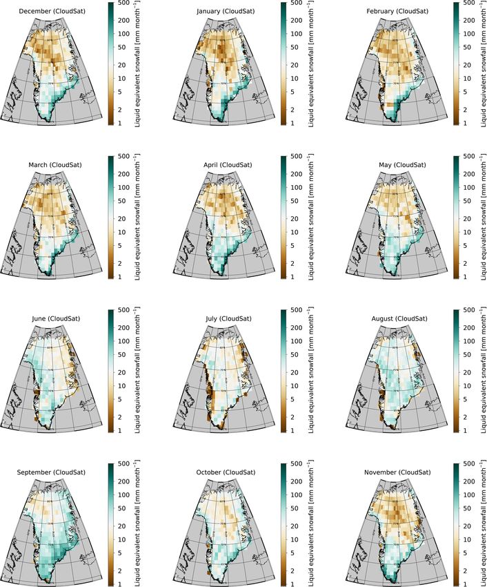
ing to the approach outlined here. This screens out cases Figures 16 and 17 show the monthly mean spatial distribu-
with high reflectivity that are associated with rainfall. tion of snowfall from CloudSat and ERA, respectively. Both
datasets identify a band near the southwest coast of Green-
These derived snowfall rates will form the basis of all further
land, where snowfall in summer is near zero. These coastal
discussion from here on.
areas are presumably too warm in summer for snow to reach
the ground before melting. Note that the CloudSat data are at
4 Comparison of CloudSat with ERA-Interim snowfall a coarser (1◦ × 2◦ ) resolution than the ERA-Interim reanaly-
climatology sis data, which explains this narrow coastal feature to be less
pronounced in CloudSat compared to ERA.
Using the strategy laid out in the previous section, we de-
rive monthly mean CloudSat estimates over the GrIS for all 4.1 Snowfall by drainage system
months where CloudSat data are available and at a resolution
of 1◦ × 2◦ , which roughly corresponds to 111 km × 111 km As can be seen in Fig. 14, even at a resolution 1◦ × 2◦ ,
at 60◦ N. In comparison, the resolution of ERA-Interim re- the monthly CloudSat precipitation estimates over the GrIS
analysis at 60◦ N is 0.7◦ × 0.7◦ or 78 km × 39 km. Figure 14 are relatively noisy. As a nadir-looking instrument, CloudSat
shows the annual mean values (calculated as a mean of only provides few overpasses per grid-box per month. In ad-
monthly means) for CloudSat (Fig. 14a) and ERA (Fig. 14b), dition to grid-box-averaged precipitation estimates, we there-
as well as their relative difference in percentage (Fig. 14c). fore also evaluate CloudSat per major GrIS drainage system.
Figure 15 shows the annual cycle over the GrIS. We first binned CloudSat data onto the 0.7◦ × 0.7◦ ERA-
Marked differences between ERA-Interim reanalysis and Interim reanalysis grid and subsequently averaged these grid-
CloudSat exist in the months June–September, where ERA ded data onto the drainage basins.
shows less precipitation over the GrIS than CloudSat. For Figures 18 and 19 show the annual cycle of precipitation
the summer months, the spatial correlation between ERA for the different major GrIS drainage areas as defined by
and CloudSat is also worst. Differences are most pronounced Zwally et al. (2012). Consistent with earlier studies (Berdahl
over the high GrIS north of 72◦ N, where ERA shows very et al., 2018), the southeast of Greenland experiences the
www.atmos-chem-phys.net/19/8101/2019/ Atmos. Chem. Phys., 19, 8101–8121, 20198114 R. Bennartz et al.: Spatial and temporal variability of snowfall over Greenland Figure 14. Annual mean liquid equivalent snowfall from CloudSat (a), ERA-Interim (2006–2016, b), and the relative difference between both (c). Figure 15. Annual cycle of liquid equivalent snowfall over the GrIS from CloudSat and ERA-Interim (a), spatial correlation between the two (b), mean bias (c), and mean relative bias (d). The dashed horizontal lines represent the annual average. highest mean snowfall, and snowfall there peaks typically (e.g., Area 1.1). In some areas on the east coast of Greenland in wintertime. We note that the snowfall values reported in (e.g., Area 3.3), the agreement between CloudSat and ERA Berdahl et al. (2018) are much higher than our estimates but is strikingly good. The agreement in these areas seems to in- also higher than other published estimates (e.g., Cullather et dicate that snowfall associated with cyclonic activity over the al., 2014). This appears to be related to Berdahl et al. (2018)’s southeast of Greenland is represented well by ERA, whereas use of only coastal stations, which experience more precip- snowfall associated with summertime precipitation is poten- itation than inland (Mira Berdahl, personal communication, tially underrepresented in the reanalysis model. 10 May 2018). In contrast, much of the northern parts of the The dashed curves in Fig. 19 are cosine fits of the an- GrIS receive very little snowfall, but peak snowfall in those nual cycle of precipitation, which are used to determine the areas is in August. These features can also be observed in months of maximum snowfall as well as the amplitude of Figs. 16 and 17. snowfall reported in Fig. 18. We note that these cosine fits do Figure 19 compares the annual cycle of snowfall between not necessarily correspond to physical features in the annual CloudSat and ERA for all drainage areas. With few excep- cycle of precipitation for all drainage systems, so the values tions, the annual cycles between CloudSat and ERA are very given for the annual cycle in Fig. 18 should not be interpreted similar. Furthermore, the summertime negative bias of ERA too quantitatively. It does appear, however, that large parts of is apparent for many of the more northern drainage areas the central and northwestern GrIS see maximum precipita- Atmos. Chem. Phys., 19, 8101–8121, 2019 www.atmos-chem-phys.net/19/8101/2019/
R. Bennartz et al.: Spatial and temporal variability of snowfall over Greenland                                8115

Figure 16. CloudSat-derived monthly mean snowfall rates.

www.atmos-chem-phys.net/19/8101/2019/                                        Atmos. Chem. Phys., 19, 8101–8121, 2019
8116                                        R. Bennartz et al.: Spatial and temporal variability of snowfall over Greenland

Figure 17. Same as Fig. 16 but for ERA-Interim.

Atmos. Chem. Phys., 19, 8101–8121, 2019                                          www.atmos-chem-phys.net/19/8101/2019/
R. Bennartz et al.: Spatial and temporal variability of snowfall over Greenland                                                        8117

Figure 18. Annual snowfall associated with the different drainage systems defined by Zwally et al. (2012). Panel (a) shows the mean annual
snowfall, panel (b) shows the fractional contribution to the total snowfall over the GrIS, panel (c) shows the month of maximum precipitation
as well as the drainage-basin identifier used in Zwally et al. (2012), and panel (d) shows the amplitude of the annual cycle of snowfall. The
month of maximum precipitation and amplitude are derived using a cosine fit to the annual cycle (see Fig. 19).

tion in summer, whereas the southeastern part of the GrIS                mates agree well with the snow stake field with the exception
sees maximum precipitation in winter.                                    of June and July, where CloudSat (as well as the MMCR)
   In the next section we further investigate the differences            report much higher snowfall accumulation than the snow
between ERA-Interim reanalysis and CloudSat based on                     stake field. A similar discrepancy between June/July stake
monthly mean snowfall accumulation over Summit, where                    field observations and other snowfall measurements was al-
independent observational data are available.                            ready reported by Dibb and Fahnestock (2004). Castellani
                                                                         et al. (2015), in their Fig. 4, show a similar behavior. No-
4.2   Annual cycle of snowfall at Summit                                 tably, June and July are the months with the highest inter-
                                                                         annual variability in snowfall. For completeness, we have
Figure 20 compares monthly mean snowfall rates over Sum-                 also included the annual cycle based on the original Cloud-
mit from all data sources discussed here. The snow stake                 Sat SNOWPROF retrieval (green). One can see that using the
field data have been corrected for sublimation/deposition us-            SNOWPROF surface snowfall rate retrieval without the cor-
ing ERA estimates and converted to liquid equivalent snow-               rections discussed and applied here would yield a precipita-
fall in order to make results directly comparable to the                 tion estimate lower than ERA and would also fail to show the
other snowfall estimates. Cullen et al. (2014) study sublima-            strong annual cycle seen in the other observational datasets.
tion/deposition over the high GrIS in detail and find the con-
tribution of sublimation/deposition to be generally around
2 % of the total accumulation. On a monthly basis, values
from ERA were a bit higher but still did not significantly
alter the snow stake field values. The CloudSat snowfall esti-

www.atmos-chem-phys.net/19/8101/2019/                                                      Atmos. Chem. Phys., 19, 8101–8121, 2019
You can also read