Identifying insects, clouds, and precipitation using vertically pointing polarimetric radar Doppler velocity spectra
←
→
Page content transcription
If your browser does not render page correctly, please read the page content below
Atmos. Meas. Tech., 14, 4425–4444, 2021
https://doi.org/10.5194/amt-14-4425-2021
© Author(s) 2021. This work is distributed under
the Creative Commons Attribution 4.0 License.

Identifying insects, clouds, and precipitation using vertically
pointing polarimetric radar Doppler velocity spectra
Christopher R. Williams1 , Karen L. Johnson2 , Scott E. Giangrande2 , Joseph C. Hardin3 , Ruşen Öktem4,5 , and
David M. Romps4,5
1 Ann  and H. J. Smead Aerospace Engineering Sciences Department, University of Colorado,
Boulder, CO, 80309, United States
2 Brookhaven National Laboratory, Upton, NY, 11973, United States
3 Pacific Northwest National Laboratory, Richland, WA, 99354, United States
4 Department of Earth and Planetary Science, University of California, Berkeley, CA, 94720, United States
5 Climate and Ecosystem Sciences Division, Lawrence Berkeley National Laboratory, Berkeley, CA, 94720, United States

Correspondence: Christopher R. Williams (christopher.williams@colorado.edu)

Received: 5 February 2021 – Discussion started: 9 February 2021
Revised: 6 May 2021 – Accepted: 6 May 2021 – Published: 16 June 2021

Abstract. This study presents a method to identify and dis-      rithms are combined in the Doppler velocity spectra domain
tinguish insects, clouds, and precipitation in 35 GHz (Ka-       and then filtered to produce a binary hydrometeor mask in-
band) vertically pointing polarimetric radar Doppler velocity    dicating the occurrence of cloud, raindrops, or ice particles
power spectra and then produce masks indicating the occur-       at each range gate. Forty-seven summertime days were pro-
rence of hydrometeors (i.e., clouds or precipitation) and in-    cessed with the insect–hydrometeor discrimination method
sects at each range gate. The polarimetric radar used in this    using US Department of Energy (DOE) Atmospheric Radia-
study transmits a linear polarized wave and receives signals     tion Measurement (ARM) program Ka-band zenith pointing
in collinear (CoPol) and cross-linear (XPol) polarized chan-     radar observations in northern Oklahoma, USA. For these
nels. The measured CoPol and XPol Doppler velocity spec-         47 d, over 70 % of the hydrometeor mask column bottoms
tra are used to calculate linear depolarization ratio (LDR)      were within ±100 m of simultaneous ceilometer cloud base
spectra. The insect–hydrometeor discrimination method uses       heights. All datasets and images are available to the public
CoPol and XPol spectral information in two separate algo-        on the DOE ARM repository.
rithms with their spectral results merged and then filtered
into single value products at each range gate. The first algo-
rithm discriminates between insects and clouds in the CoPol
Doppler velocity power spectra based on the spectra tex-         Copyright statement. This paper has been authored by employees
ture, or spectra roughness, which varies due to the scatter-     (Karen L. Johnson and Scott E. Giangrande) of Brookhaven Science
                                                                 Associates, LLC, under contract No. DE-SC0012704 with the US
ing characteristics of insects vs. cloud particles. The second
                                                                 Department of Energy (DOE). The publisher by accepting the paper
algorithm distinguishes insects from raindrops and ice parti-    for publication acknowledges that the United States Government
cles by exploiting the larger Doppler velocity spectra LDR       retains a nonexclusive, paid-up, irrevocable, worldwide license to
produced by asymmetric insects. Since XPol power return          publish or reproduce the published form of this paper, or allow oth-
is always less than CoPol power return for the same target       ers to do so, for United States Government purposes.
(i.e., insect or hydrometeor), fewer insects and hydromete-
ors are detected in the LDR algorithm than the CoPol algo-
rithm, which drives the need for a CoPol based algorithm.
After performing both CoPol and LDR detection algorithms,
regions of insect and hydrometeor scattering from both algo-

Published by Copernicus Publications on behalf of the European Geosciences Union.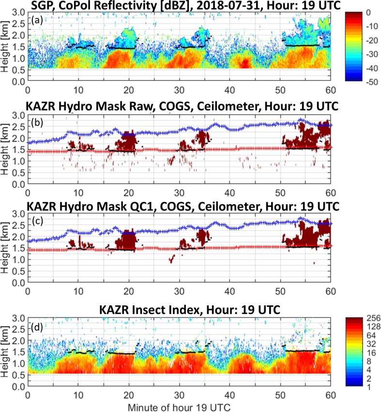
4426 C. R. Williams et al.: Identifying insects, clouds, and precipitation
1 Introduction has been used to distinguish insect and hydrometeor peaks
in Doppler velocity spectra (Bauer-Pfundstein and Görsdorf,
The vertical structure of non-precipitating clouds plays an 2007; Luke et al., 2008). In these studies, multiple peaks
important role in the Earth’s radiation balance. These clouds were first found in the spectra and then intelligent algorithms
absorb longwave radiation emitted from the surface and re- (Bauer-Pfundstein and Görsdorf, 2007) or neural network al-
flect shortwave solar radiation back into space (Cess et al., gorithms (Luke et al., 2008) were developed to classify peaks
1990). The proportion of these two processes determines as the result of either insect or hydrometeor scattering. The
whether these clouds act as a net radiation sink or source in method presented herein reverses the processing steps by
the Earth’s radiation budget (Ramanathan et al., 1989). Ver- first identifying and then removing insect signatures in the
tically pointing cloud radars have been used for decades to Doppler velocity spectra before estimating spectrum peaks.
quantify the extent to which non-precipitating clouds can be Identifying and removing radar scattering from insects and
used as inputs to Earth radiation budget studies to understand other sources of “atmospheric plankton” (Lhermitte, 1966)
cloud dynamics and cloud lifecycles (Moran et al., 1998; has been a known problem in developing operational cloud
Ackerman and Stokes, 2003). products (Kollias et al., 2016). The US Department of Energy
In addition to measuring cloud properties, cloud radars are (DOE) Atmospheric Radiation Measurement (ARM) pro-
sensitive enough to detect individual insects within the radar gram merges observations from multiple sensors (including
volume (for overviews, see Riley, 1989; Westbrook et al., radars, lidars, and ceilometers) to produce an estimate of hy-
2014; Nansen and Elliot, 2016). The field of radar entomol- drometeors (i.e., cloud particles, raindrops, and ice particles)
ogy exploits this sensitivity by pointing polarimetric radar in the vertical column, called the Active Remote Sensing of
beams a few degrees off vertical and rotating the beam 360◦ CLouds (ARSCL) product (Clothiaux et al., 2000). ARSCL
in azimuth to estimate insect population and migration direc- is a high temporal (∼ 4 s) and vertical (∼ 30 m) resolution op-
tion (Drake et al., 2020). The field of radar meteorology has erational product that primarily uses ceilometer cloud base
used polarimetric scanning radar observations to track insect and radar moments to classify all returns into one of three
flying direction and altitude outside of clouds (Mueller and scattering regimes: hydrometeor-only scattering, clutter-only
Larkin, 1985) and to estimate gust-front motions ahead of scattering (due to insects or another non-atmospheric arti-
convective cells because insects and small pieces of vegeta- fact), and scattering due to a mixture of hydrometeors and
tion act as radar reflectors trapped within the strong bound- clutter within the radar pulse volume. An approximate esti-
ary layer outflow (Klingle et al., 1987). Insects are con- mate of maximum clutter height is provided to an automated
sidered clutter and unwanted signals in vertically pointing heuristic algorithm developed over two decades of experi-
cloud radar observations. Two approaches have been used ence producing the ARSCL product at multiple radar sites.
to identify insects in cloud radar observations: polarimet- The results of the classification are reviewed. On rare occa-
ric signatures and Doppler velocity power spectra signa- sions, the maximum clutter height is revised and the classifi-
tures. Compared to more spherical hydrometeors (i.e., cloud cation procedure is repeated.
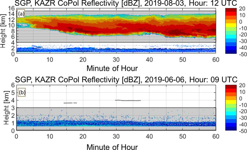
droplets, raindrops, and ice particles), insects have asymmet- Figure 1 shows 1 h of ARSCL processed reflectivity from
rical shapes that produce large cross-polarization power re- the DOE ARM Southern Great Plains (SGP) central facility
turn signals that enable insects to be identified with polari- on 31 July 2018 (ARM user facility, 2014). Figure 1a (top
metric radar estimates including differential reflectivity and panel) shows ARSCL reflectivity for radar volumes classi-
linear depolarization ratio (Lohmeier et al., 1997; Sekelsky et fied as either hydrometeor-only or hydrometeor-plus-clutter
al., 1998; Khandwalla et al., 2001, 2002; Martner and Moran, with Fig. 1b (middle panel) showing ARSCL hydrometeor-
2001). Also, large insects will have different radar cross sec- only reflectivities. The black symbols represent ceilometer-
tions at different radar operating wavelengths due to the res- derived cloud base, which is also an input to the ARSCL
onance or Mie scattering effects enabling insects to be de- operational algorithm. Figure 1c (bottom panel) shows the
tected in dual-wavelength radar observations (Khandwall et hydrometeor mask produced using the algorithms discussed
al., 2001, 2002; Kollias et al., 2002). herein. The apparent fall streaks in the ARSCL hydrometeor-
Insects produce unique signatures in the Doppler veloc- only product below 1.5 km are misclassifications of insect
ity power spectra. An individual insect scatters as a sin- clutter. The misclassification of insect clutter as hydromete-
gle point target with a returned power confined to a narrow ors and the inefficient ARSCL processing steps were some
Doppler velocity range and to a single range gate (Bauer- of the reasons why DOE ARM sponsored this work to iden-
Pfundstein and Görsdorf, 2007). In contrast, clouds and pre- tify insect clutter with the aim of improving future ARSCL
cipitation are composed of hydrometeor distributions con- products.
taining different size particles with different velocities that The method to identify insects and hydrometeors pre-
are spread over several range gates leading to broader mea- sented herein builds on prior work using polarimetric di-
sured Doppler velocity power spectra extending over several versity and Doppler velocity power spectra variability (e.g.,
range gates (Luke et al., 2008). The difference between insect Martner and Moran, 2001; Bauer-Pfundstein and Görsdorf,
and hydrometeor Doppler velocity power spectra signatures 2007; Luke et al., 2008; Görsdorf et a., 2015). One unique
Atmos. Meas. Tech., 14, 4425–4444, 2021 https://doi.org/10.5194/amt-14-4425-2021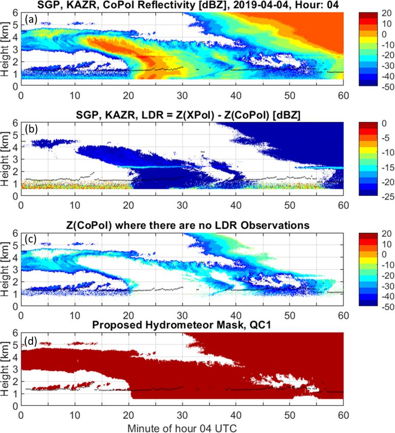
C. R. Williams et al.: Identifying insects, clouds, and precipitation 4427
(SGP) central facility located in northern Oklahoma. Verti-
cally pointing Ka-band radar co-polarized (CoPol) and cross-
polarized (XPol) Doppler velocity power spectra are pro-
cessed to identify insects, clouds, and precipitation in the ver-
tical column. Verification of those classifications are based
on observations from co-located lidar, ceilometer, Total Sky
Imager (TSI), and cloud boundaries contained in the Clouds
Optically Gridded by Stereo (COGS) product (Romps and
Öktem, 2018).
2.1 Ka-band ARM zenith pointing radar (KAZR)
The DOE ARM program deploys atmospheric observing
systems to characterize the radiative properties of clouds
in the atmosphere (Mather and Voyles, 2013). One of
ARM’s hallmark instruments is the Ka-band (35 GHz)
ARM zenith pointing cloud radar (KAZR), which trans-
mits linear polarized waves that are detected simultane-
ously with collinear polarized (CoPol) and cross-linear polar-
Figure 1. Active Remote Sensing of CLouds product (ARSCL) for ized (XPol) receivers. The received signals are processed to
hour 19:00 UTC (14:00 LT) from the DOE ARM Southern Great CoPol (v , h ) (Watts) and cross-polarized
yield co-polarized Ssignal i j
Plains (SGP) central facility on 31 July 2018. (a) ARSCL reflec- XPol
Ssignal (vi , hj ) (Watts) Doppler velocity power at each veloc-
tivity for radar volumes ARSCL classified as either hydrometeor-
only or hydrometeor-plus-clutter. (b) ARSCL reflectivity for radar ity bin vi and range gate hj . The linear depolarization ratio
spectra profile SdB LDR (v , h ) (dB) is the ratio of polarized sig-
volumes ARSCL classified as hydrometeor-only. (c) Hydrometeor i j
mask produced using the method described herein. The black sym- nal magnitudes defined as
bols in all panels are ceilometer-derived cloud base. Note the hy- " XPol #
drometeor misclassification below the ceilometer cloud base in (b) LDR
Ssignal vi , hj
SdB vi , hj = 10 log CoPol (1a)
motivates the need for improved insect clutter detection. Ssignal vi , hj
or as
feature of the proposed algorithms is that insect and hydrom- LDR
SdB
XPol
vi , hj = Ssignal,dB
CoPol
vi , hj − Ssignal,dB (vi , hj ), (1b)
eteor scattering are identified before identifying significant
peaks in the Doppler velocity spectra. This approach comple- XPol
where Ssignal,dB CoPol (v , h ) are expressed
(vi , hj ) and Ssignal,dB i j
ments the methods that first identify multiple peaks and then in decibel units (dB) using XdB = 10 log [X]. The linear de-
classify each peak (Bauer-Pfundstein and Görsdorf, 2007; polarization ratio LDR (dB) is the integration of XPol and
Luke et al., 2008). The observations used in this study and the CoPol signals over the spectrum and is defined as
signatures of insect and hydrometeor scattering are discussed v XPol
max S
in Sects. 2 and 3. Section 4 presents the main concept behind P signal (vi ,hj )
CoPol 1v
the algorithms developed in this study. Section 5 compares vmin Ssignal (vi ,hj )
LDR(hj ) = 10 log , (2)
the hydrometeor masks with the Clouds Optically Gridded vP
max
by Stereo (COGS) product (Romps and Öktem, 2018) de- 1v
vmin
rived from stereo cameras. Section 5 also compares the hy-
drometeor mask cloud bottom with ceilometer-derived cloud where vmin to vmax define the velocity range of valid
base. Conclusions and next steps are discussed in Sect. 6. The CoPol (v , h ) and S XPol (v , h ) observations.
Ssignal i j signal i j
Supplement contains images of insect and hydrometeor clas- At SGP, KAZR operates in the general (GE) and medium
sifications for 47 summertime days in northern Oklahoma, (MD) sensitivity modes to sense clouds at different altitudes
USA, identified as LASSO cloud simulation events (LASSO, with operating parameters during 2018 and 2019 shown in
2020). Table 1 (ARM user facility, 2011a, b; Widener et al., 2012).
Even though insects are detected in both KAZR operating
modes, to simplify the figures and algorithm descriptions, the
2 Observations results from just the MD mode are presented herein. Since
the MD mode transmits a long frequency-modulated pulse,
The observations used in this study were collected by the the first resolved range gate is 570 m above the radar. The
US Department of Energy (DOE) Atmospheric Radiation KAZR 3.05 m diameter Cassegrain parabolic reflector man-
Measurement (ARM) program at their Southern Great Plains ufactured by Millitech produces a 0.2◦ antenna beamwidth
https://doi.org/10.5194/amt-14-4425-2021 Atmos. Meas. Tech., 14, 4425–4444, 2021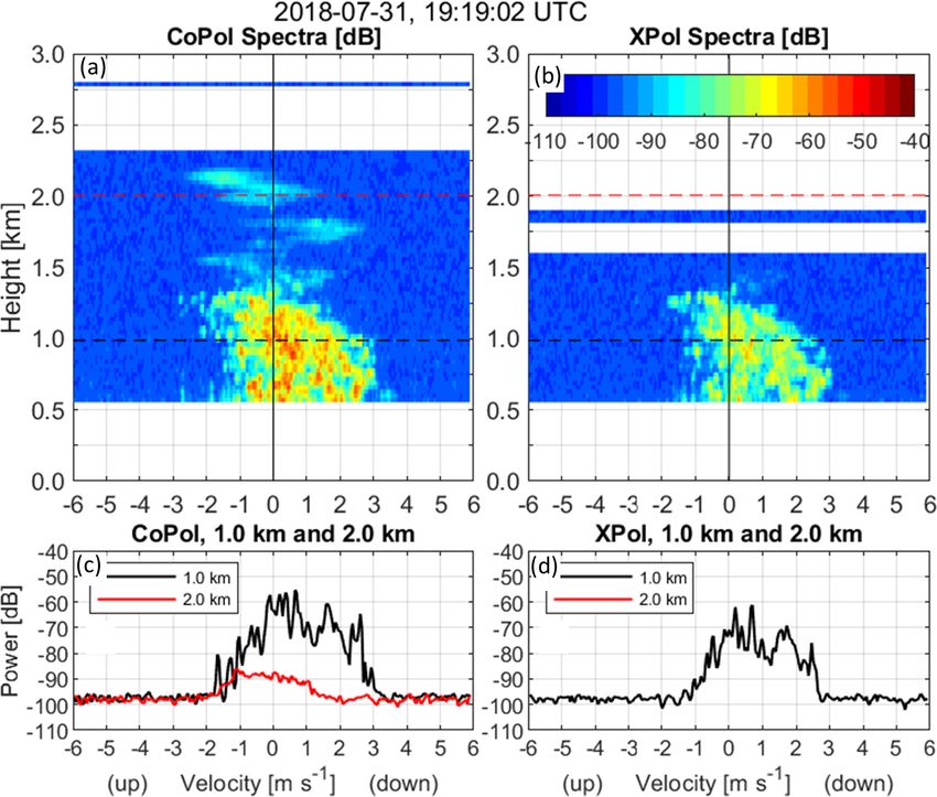
4428 C. R. Williams et al.: Identifying insects, clouds, and precipitation
Table 1. Operating parameters for KAZR deployed at ARM Southern Great Plains (SGP) during 2018 and 2019. Operating modes included
general purpose (GE) and medium sensitivity (MD) modes. Tabulated parameters include: pulse repetition frequency (PRF) (Hz), inter-pulse
period (IPP) (µs), number of points in FFT (NFFT ), number of averaged spectra (also known as number of incoherent integrations) (Nincoh ),
Nyquist velocity (VNyquist ) (m s−1 ), velocity resolution (1v) (m s−1 ), range to first range gate (m), range resolution (m), time on target
(which is calculated using IPPNFFT Nincoh ) (s), and time between samples (s).
Parameter
Sensitivity mode General (GE) Medium (MD)
Frequency (GHz) 34.83 34.89
Pulse repetition frequency (PRF) (Hz) 2771 2771
Inter-pulse period (IPP) (µs) 360 360
Pulse duration (ns) 300 3967
Pulse modulation None Linear frequency modulation
Range resolution 1R (m) 45 45
Distance between range gates (m) 30 30
Range to first range gate R1 (m) 100 570
Number of points in FFT (NFFT ) 256 256
VNyquist (m s−1 ) 5.96 5.95
1v (cm s−1 ) 4.67 4.67
Number of incoherent integrations (Nincoh ) 20 20
Time on target ttarget = IPPNFFT Nincoh (s) 1.8 1.8
Time between samples tsample (s) 3.7 3.7
with 57.5 dBi gain, has −27 dB cross-polarization isolation, 3 Insect, cloud droplet, and precipitation spectral
and has a membrane radome sloping across the antenna with characteristics
a dry two-way loss less than 2 dB (Widener et al., 2012).
The MD mode uses a non-linear frequency modulated chirp This section discusses the scattering characteristics of in-
over a 3967 ns pulse length to produce a 45 m range resolu- sects, atmospheric plankton, clouds, and precipitation as ob-
tion sampled at 30 m range spacing. At 1 km range, the radar served in KAZR CoPol and XPol Doppler velocity power
pulse volume is a 3.6 m diameter horizontal disk over a 45 m spectra. The first subsection discusses characteristics when it
range to yield a pulse volume of approximately 450 m3 . To is not raining and the radar is observing individual insects or
save computer hard disk space, the KAZR CoPol and XPol other atmospheric plankton particles scattering as point tar-
Doppler velocity power spectra are retained only at range gets with narrow velocity ranges and shallow cumulus clouds
gates with significant power above a noise threshold. scattering as distributed targets with broader velocity ranges.
The variability of return power across the Doppler velocity
2.2 Validation observations spectrum, or the spectrum “texture”, is used to distinguish
point target insects from distributed target clouds. The sec-
Two observational datasets are used to validate the derived ond subsection describes the characteristics when individual
KAZR insect and hydrometeor classifications: ceilometer insects and raindrop or ice particle distributions occur simul-
cloud base estimates from a Vaisala model CL31 ceilome- taneously in the radar volume. The LDR at each Doppler ve-
ter (ARM user facility, 2010; Morris, 2016) and cloud bot- locity bin is used to distinguish high LDR insects from low
tom and top estimates from the COGS product (ARM user LDR raindrops or ice particles.
facility, 2017). The Vaisala ceilometer uses a pulsed InGaAs
diode laser at 910 nm wavelength and the vendor-supplied 3.1 Insects and shallow cumulus clouds
algorithm estimates cloud base at 10 m and 16 s resolution
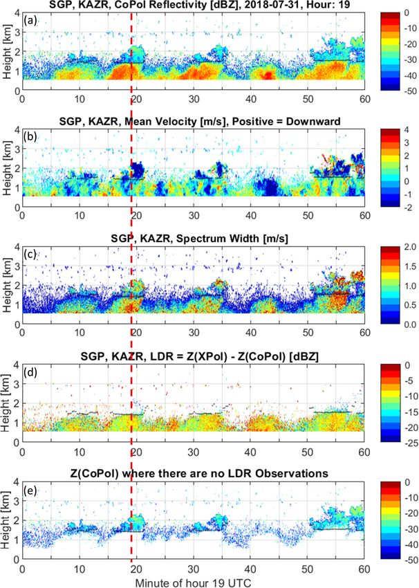
when the vertical visibility is less than 100 m (Morris, 2016). Figure 2 shows an hour of KAZR observations when insects
The COGS cloud boundaries are derived from three pairs of (or other atmospheric plankton particles) and shallow cu-
stereo cameras positioned around the SGP central facility and mulus clouds are observed over the radar during 19:00 UTC
represent cloud boundaries over a cubic domain 6 km to a (14:00 LT) on 31 July 2018. From top to bottom, Fig. 2 shows
side (Romps and Öktem, 2018). Due to camera visual occlu- KAZR (a) CoPol reflectivity (dBZ), (b) mean Doppler ve-
sion during precipitation, COGS cloud boundaries are only locity (m s−1 ), (c) Doppler velocity spectrum width (m s−1 ),
estimated for cases of shallow cumulus clouds, which allow (d) linear depolarization ratio (LDR) (dB), and (e) KAZR
the three cameras to view the vertical extent of each cloud. CoPol reflectivity at time–height locations (also called “pix-
Likewise, estimates from COGS are only available during els” in this study) that do not have an LDR measurement.
daylight hours. The black symbols in each panel indicate ceilometer-derived
Atmos. Meas. Tech., 14, 4425–4444, 2021 https://doi.org/10.5194/amt-14-4425-2021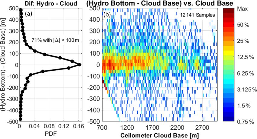
C. R. Williams et al.: Identifying insects, clouds, and precipitation                                                          4429

cloud base height, which is near 1.5 km for this hour. Below
cloud base, reflectivity (Fig. 2a) and spectrum width (Fig. 2c)
have a coherent pattern, but vertical motion (Fig. 2b) appears
more variable. If drizzle or rain were below cloud base, then
all three quantities would be coherent with downward mo-
tions increasing as reflectivity and spectrum width increase
(Williams and Gage, 2009). Thus, it is not raining below
cloud base. Above the ceilometer-derived cloud base height,
there are CoPol reflectivity observations (Fig. 2a) but not as
many LDR estimates (Fig. 2d). For example, near minute
20, there is an enhancement of CoPol reflectivity above the
ceilometer cloud base and extending above 2 km; yet, there
are very few LDR observations in this time–height region.
Since LDR requires both CoPol and XPol reflectivity ob-
servations, the lack of LDR above cloud base indicates that
the XPol channel is not detecting cloud particles. This CoPol
vs. XPol sensitivity is illustrated in the bottom panel, which
shows CoPol reflectivity for all pixels that do not also have
an LDR observation. The continuous time–height CoPol re-
flectivity observations above 1.5 km are cloud features that
are easily discernible by eye. Return signals from individual
insects appear as speckles up to 4 km in all panels.
   The CoPol and XPol Doppler velocity power spectra pro-
duced by individual insects and by cloud droplet distribu-
tions have different characteristics as illustrated in Fig. 3,
which shows CoPol (Fig. 3a) and XPol (Fig. 3b) Doppler
velocity power spectral density profiles at 19:19:02 UTC on
31 July 2018. The vertical axis extends from 0 to 3 km in
height and the horizontal axis extends ±6 m s−1 radial veloc-
ities. The Nyquist velocity is 5.95 m s−1 and downward mo-        Figure 2. Moments calculated from raw spectra for hour 19:00 UTC
tions have positive values consistent with positive raindrop      on 31 July 2018. (a) CoPol reflectivity (dBZ). (b) Mean radial
diameters having positive fall speeds due to gravity. Due to      velocity (m s−1 ); positive values are downward motion. (c) Spec-
the long coded transmitted pulse, the first observations oc-      trum width (m s−1 ). (d) Linear depolarization ratio (LDR) (dB).
cur at 0.57 km range. The colors represent the return signal      (e) CoPol reflectivity (dBZ) at pixels that do not have an LDR mea-
power expressed in dB with warmer colors indicating larger        surement. The black symbols in all panels are ceilometer-derived
return signal power. The mean noise power is approximately        cloud base. The vertical dashed line indicates time 19:02 UTC,
−100 dB.                                                          which is the time of the profile shown Figs. 3 and 6.
   Figure 3c shows CoPol Doppler velocity power spectra
at 1 and 2 km heights (black and red lines, respectively).
The power spectrum at 1 km has more variability between           profile. Shown in sequential spectra profiles in the Supple-
velocity bins compared to the spectrum at 2 km. This vari-        ment, point enhancements often appear in only one spectra
ability is because the radar is detecting individual insects      profile and not in neighboring profiles separated 4 s apart.
within the 450 m3 field of view with each insect moving at        The surface wind speed was about 3 m s−1 for this profile
its own radial velocity. If an insect is the only insect mov-     and there is not enough information to determine whether the
ing at a particular velocity, the spectrum will have an iso-      insects are passive tracers advecting with the wind or self-
lated peak (e.g., near −1.7 m s−1 radial velocity in Fig. 3c).    propelling themselves through the 3.6 m diameter by 45 m
If multiple insects are moving at similar speeds, the spec-       field of view in less than 4 s.
trum will be broader yet still have variability. For example,        In contrast to individual insects, clouds and precipitation
between −1 and +3 m s−1 radial velocities, the 1 km height        are distributed targets filling the radar volume with hundreds
spectrum (black line) is both elevated in magnitude and has       or thousands of hydrometeors of different sizes with differ-
more bin-to-bin variability than the spectrum from 2 km (red      ent radial velocities. Since the number of particles in the hy-
line). Also, the backscattered power from insects is primar-      drometeor size distribution varies gradually over neighbor-
ily confined to one range gate with some power leaking into       ing particle sizes and the hydrometeor spectrum is extended
neighboring range gates due to radar signal processing lim-       in the velocity dimension due to antenna broadening effects,
itations, which produce point enhancements in the spectra         the return power spectrum has a gradual change over neigh-

https://doi.org/10.5194/amt-14-4425-2021                                             Atmos. Meas. Tech., 14, 4425–4444, 2021
4430                                                          C. R. Williams et al.: Identifying insects, clouds, and precipitation

Figure 3. Spectra from the profile at 19:19:02 UTC on 31 July 2018.
(a) CoPol Doppler velocity power spectra (dB) as a function of
range and radial velocity. (b) XPol Doppler velocity power spectra
(dB) as a function of range and radial velocity. (c) CoPol Doppler
velocity power spectra at 1.0 km (black line) and 2.0 km (red line).
(d) XPol Doppler velocity power spectra at 1.0 km (black line).
                                                                       Figure 4. Moments calculated from raw spectra and the retrieved
                                                                       hydrometeor QC1 mask for hour 04:00 UTC on 4 April 2019.
                                                                       (a) CoPol reflectivity (dBZ). (b) Linear depolarization ratio (LDR)
boring velocity bins. Thus, the power spectrum from a dis-             (dB). (c) CoPol reflectivity (dBZ) at pixels that do not have an LDR
tribution of many hydrometeors is smoother than the return             measurement. (d) Retrieved hydrometeor QC1 mask. The black
from a few individual insects. The smoother power spectra              symbols in both panels are ceilometer-derived cloud base.
at 2 km height shown in Fig. 3c are consistent with a distri-
bution of small cloud droplets moving at different velocities
within the radar volume. In addition to smooth power spec-             enhancement near 2.4 km and after minute 20 is due to a
tra across the velocity dimension, power spectra from cloud            mixture of liquid and frozen particles near the melting layer
droplets are also more continuous in range due to the vertical         (Baldini and Gorgucci, 2006). Below the melting layer, the
extent of clouds as can be seen with a continuity of clouds            LDR has values near −25 dB that is due to scattering from
with height in Fig. 3a.                                                raindrops. Above the melting layer, scattering from asym-
                                                                       metrical ice particles leads to LDR values near −20 dB (Bal-
3.2    Insects and precipitation                                       dini and Gorgucci, 2006). In contrast to the shallow cumu-
                                                                       lus cloud droplet observations in Figs. 2 and 3, KAZR has
Figure 4 shows time–height cross sections of KAZR CoPol                enough sensitivity to detect XPol signal returns from large
reflectivity (Fig. 4a) and LDR observations (Fig. 4b)                  spherical raindrops and ice particles.
when insects, clouds, and precipitation are observed in the               Figure 4c shows the CoPol reflectivity at time–height pix-
same hour. Observations were collected during 04:00 UTC                els that do not have an LDR measurement. As with the
(23:00 LT) on 4 April 2019. From minutes 0–20, the approx-             shallow cloud observations (see Fig. 2e), there are more
imate 1.5 km ceilometer cloud base height (black symbols) is           CoPol observations than LDR observations. The bottom
above the insect layer that has LDR values between approxi-            panel (Fig. 4d) shows the QC1 hydrometeor mask produced
mately −5 and −10 dB (see Fig. 4b), while the CoPol reflec-            by the insect–hydrometeor detection algorithm described in
tivity is continuous in time and height above the ceilometer           Sect. 4. The events shown in Figs. 2–4 highlight three impor-
cloud base height (see Fig. 4a and c). At the beginning of the         tant attributes of CoPol and LDR measurements:
hour, the CoPol reflectivity (Fig. 4a) time–height structure
indicates a precipitating cloud system between 3 and 5 km                – LDR measurements detect some, but not all, insect,
that evolves in time with precipitation reaching the lowest                cloud, and precipitation observations.
resolved height of 0.57 km after minute 20. The LDR shows
a similar time–height structure (with reduced vertical depth)            – KAZR LDR measurements do not have the sensitivity
with LDR values ranging between −25 to −20 dB. The LDR                     to detect shallow non-precipitating liquid clouds.

Atmos. Meas. Tech., 14, 4425–4444, 2021                                                  https://doi.org/10.5194/amt-14-4425-2021
C. R. Williams et al.: Identifying insects, clouds, and precipitation                                                                4431

    – Doppler velocity power spectra contain signatures               variability than cloud droplet or raindrop distributions. The
      unique to insect scattering and hydrometeor scattering.         LDR algorithm classifies insects and hydrometeors based
                                                                      on the understanding that asymmetric insects produce larger
The limitation of LDR measurements not detecting all insects
                                                                      LDR magnitudes than spherical raindrops (when viewed
detected by CoPol measurements and the benefit of Doppler
                                                                      from the bottom) and that the non-precipitating liquid cloud
velocity power spectra having signatures of insects and hy-
                                                                      droplets should not produce any signal in the KAZR XPol
drometeor scattering suggests that Doppler velocity power
                                                                      channel for single scattering processes. Both algorithms pro-
spectra can be analyzed along with LDR measurements to
                                                                      duce insect–hydrometeor membership classes for every re-
discriminate between insect and hydrometeor scattering.
                                                                      gion of the spectra profile. The membership classes are com-
                                                                      bined and then reduced to binary insect and hydrometeor
4     Anatomy of insect–hydrometeor detection algorithms              masks that have affirmative values for insect or hydrome-
                                                                      teor scattering at each range gate. After processing individ-
As described previously, the radar returned signal re-                ual spectra profiles, two time–height continuity quality con-
sults from scattering from insects (including atmospheric             trol (QC) filters are applied to the binary hydrometeor masks
plankton) and/or hydrometeors (aka, cloud droplets or                 to remove outliers. This is based on the understanding that
precipitation-sized particles). The insect–hydrometeor detec-         clouds and precipitation are persistent over tens of seconds
tion algorithms described in this section aim to classify each        and tens of meters. Details of each algorithm module are de-
region of the CoPol and LDR Doppler velocity spectra as ei-           scribed in the following sections.
ther insect or hydrometeor scattering. Next, the two CoPol
and LDR regional spectral classifications are combined and            4.1   CoPol texture algorithm branch
then filtered to produce masks indicating the occurrence of
insect or hydrometeor scattering at every range gate.                 This section describes the CoPol texture algorithm by apply-
   The detection algorithms start with the observed CoPol             ing the processing steps (Boxes 1–4 of Fig. 5) to the observed
and XPol spectra profiles Sobs  CoPol/XPol (v , h ) (Watts). These
                                             i j                      spectra profile shown in Fig. 3a. An objective noise thresh-
                                        CoPol/XPol (v , h ) (Watts)
are a combination of signal power Ssignal            i j              old nHS (hj ) is estimated from the CoPol spectra at each
and random noise power n(vi , hj ) (Watts)                            height (Hildebrand and Sekhon, 1974; Carter et al., 1995).
                                                                      The CoPol spectra with magnitudes greater than nHS (hj )
  CoPol             CoPol

Sobs     vi , hj = Ssignal vi , hj + n vi , hj                (3a)    are defined as signal power (see Eq. 3). The CoPol signal
                                                                      power for the boundary layer spectra in Fig. 3a is shown in
and
                                                                      Fig. 6a. As discussed before, insect scattering produces delta
 XPol            XPol

Sobs  vi , hj = Ssignal vi , hj + n vi , hj .                 (3b)    functions in the power spectra that are broadened in the ve-
                                                                      locity domain because of hardware limitations (e.g., antenna
The signal powers are a combination of insect signal power            beamwidth) and signal processing techniques (e.g., FFT pro-
 CoPol/XPol (v , h ) (Watts) and hydrometeor signal power
Sinsect        i j
 CoPol/XPol (v , h ) (Watts) for both polarizations. This can
                                                                      cessing). A texture parameter T dB (vi , hj ) (dB) (Box 2 of
Shydro         i j                                                    Fig. 5) captures delta function variability in the CoPol power
be expressed as                                                       spectra and is defined as
 CoPol               CoPol            CoPol

Ssignal vi , hj = Sinsect  vi , hj + Shydro vi , h j     (4a)                            h
                                                                      T dB vi , hj =max Ssignal,dB
                                                                                             CoPol              CoPol

                                                                                                      (vi ) − Ssignal,dB (vi−1 ) ,
and                                                                                                                        i
                                                                                      CoPol               CoPol
 XPol
                  XPol
                                    XPol
                                                                                    Ssignal,dB (vi ) − Ssignal,dB (vi+1 ) ,          (5)
Ssignal vi , hj = Sinsect vi , hj + Shydro vi , h j .         (4b)
The goal of the CoPol and LDR insect–hydrometeor detec-               where max[a, b] selects the larger magnitude value between
tion algorithms is to classify insect and hydrometeor scatter-        estimates a or b. To capture both positive and negative
ing contributions at each (vi , hj ) location. Insects and hy-        changes equally, T dB (vi , hj ) uses the absolute magnitude,
drometeors do occur in the same range gate and sometimes              then selects the largest difference between the neighbors (i.e.,
at the same velocity (as will be seen in Figs. 6, 8, 9, and           vi−1 or vi+1 ). Figure 6b shows the texture T dB (vi , hj ) for the
11). These simultaneous insect and hydrometeor classifica-            CoPol power spectra shown in Fig. 6a. Note that the small
tions will be mitigated by temporal quality control filtering.        magnitude texture values in the upper heights are due to
   The observed KAZR CoPol and XPol spectra profiles                  cloud droplet scattering and larger magnitude texture values
(Fig. 3) are the inputs to the insect–hydrometeor algorithms,         in the lower heights are caused by insect scattering. Several
with the processing steps for both algorithms outlined in             features make texture T dB (vi , hj ) well suited for identifying
Fig. 5. The methodology consists of two parallel algorithms.          insect produced delta function variability. First, the texture
The CoPol texture algorithm classifies insects and hydrom-            T dB (vi , hj ) is calculated using signal powers expressed in
eteors based on the CoPol spectra texture, with the under-            decibel units. Thus, the power difference between neighbors
standing that scattering from insects produces more spectrum          in decibel units is the same as a power ratio, or a percent

https://doi.org/10.5194/amt-14-4425-2021                                                 Atmos. Meas. Tech., 14, 4425–4444, 2021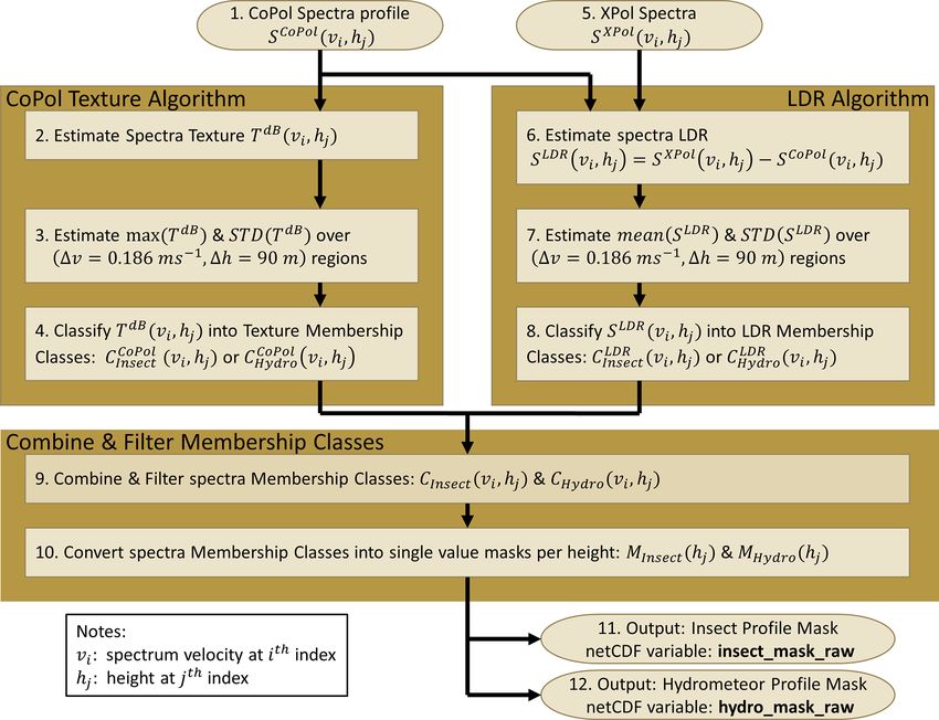
4432                                                        C. R. Williams et al.: Identifying insects, clouds, and precipitation

Figure 5. Retrieval logical flow diagram.

change, Awhen
               the power is expressed in linear units (e.g.,        ible near 1.8 and 2 km indicating that insect scattering is oc-
10 log B    = 10 log[A]−10 log[B]). This implies that fluctu-        curring with close proximity to cloud scattering regions.
ations expressed in decibel units are independent of magni-             With an objective of separating insect and cloud scatter-
tude, which allows for comparisons of low magnitude cloud            ing regions based on CoPol texture statistics, Fig. 7a, b, and
observations with larger magnitude insect observations as            c shows one-dimensional (1D) and two-dimensional (2D)
shown in Fig. 3. Second, a narrow KAZR antenna beamwidth             probability distribution                          dB        dB
                                                                            dB
                                                                                         dB  functions (PDFs) of TSD = SD T
allows the difference between nearest neighbors (i.e., vi and        and Tmax = max T          for all profiles in hour 19:00 UTC of
vi±1 ) to quantify delta functions. Note that depending on           31 July 2018 and all spectral regions that do not have an LDR
radar hardware and operating parameters, the insect peak             measurement. The spectral regions with an LDR measure-
may be broader than these observations, and power differ-            ment are shown in Fig. 7d, e, and f. The color coding in the
ences using further neighbors may be necessary in order to           2D plot represents the percent occurrence relative to the cell
identify delta functions (e.g., between vi and vi±2 ).               with the maximum number of observations. The 1D PDFs
   With a goal of identifying regions of insect and hy-              produced from the observations are shown with black curves
drometeor scattering, a small velocity–height window is              in Fig. 7a and c using 953 136 samples, each representing a
moved throughout the T dB (vi , hj ) domain and texture statis-      small spectral region, distributed    into two populations.
                                                                                                                              The
                                                                     peak with smaller SD T dB and smaller max T dB is due

tics are calculated for each small region. For this KAZR
dataset, a velocity–height window of five velocity bins              to cloud particle scattering. The peak with larger texture at-
(total width of 0.186 m s−1 ) and three range gates (to-             tributes is caused by insect scattering. The contour lines in
tal depth of 90 m) was large enough to capture regional              Fig. 7b represent 90 %, 75 %, 63 %, and 50 % occurrence of
texture variability. For each small region, maximum tex-           2D Gaussian functions estimated for both populations. The
        dB = max T dB (v
ture Tmax                    i±2 ,hj ±1 ) and standard deviation    red lines in Fig. 7a and c are 1D Gaussian function fits to
  dB = SD T dB (v

TSD                  i±2 j ±1 ) are estimated and assigned to
                         , h                                         the observations. Better fits were obtained using generalized
the location (vi , hj ). Figure 6c and d show the regional max-      Gaussian functions that accounted for skewness in the ob-
imum and standard deviation for the texture shown in Fig. 6b.        served distributions. However, these better fits did not yield
Note that both quantities are larger at lower altitudes where        better classifications, as better classifications depend on the
insect scattering dominates compared to higher altitudes that        samples between the two peaks and not on the outer tails of
are dominated by cloud droplet scattering. Interestingly, en-        the distributions that determined the distribution skewness.
hancements in both maximum texture and SD texture are vis-              The observations with LDR in Fig. 7d, e, and f show only
                                                                     one distribution corresponding to insect scattering. The func-

Atmos. Meas. Tech., 14, 4425–4444, 2021                                               https://doi.org/10.5194/amt-14-4425-2021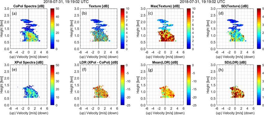
C. R. Williams et al.: Identifying insects, clouds, and precipitation                                                                      4433

Figure 6. Spectra profile measurements and calculations from the profile at 19:19:02 UTC on 31 July 2018. (a) CoPol spectra. (b) CoPol tex-
ture. (c) Max(texture). (d) SD(texture). (e) XPol spectra. (f) LDR spectra. (g) Mean(LDR). (h) SD(LDR). All measurements and calculations
are in units of dB.

Figure 7. 1D and 2D distributions of texture statistics from hour 19:00 UTC on 31 July 2018. Panels (a)–(c) are 953 136 spectra regions
without LDR detected and panels (d)–(f) are 972 113 spectra regions with LDR detected. (a) 1D PDF of SD(texture). The black line is
observations and the red dashed line is fit to two Gaussian distributions. (b) Colors are the observed 2D distribution of SD(texture) vs.
Max(texture). Colors represent the percentage of occurrence relative to the cell with the maximum number of observations. Blue and red
contours are 2D Gaussian fits to hydrometeors (blue) and insects (red). Contours represent 90 %, 75 %, 63 %, and 50 % occurrence. Gaussian
fit parameters are displayed in panel (b). The threshold between hydrometeor and insect is indicated by the dashed black line. (c) 1D PDF of
Max(texture). The black line is observations and the red line is fit to two Gaussian distributions. (d) Similar to (a) except for spectra regions
with detected LDR. (e) Similar to (b) except there is only one distribution caused by insect scattering. Contours are 2D generalized Gaussian
fits. (f) Similar to (c) except the red curve is fit to one generalized Gaussian distribution.

tional fits are generalized Gaussian distributions and capture             2.7 dB standard deviations). Also note that the insect distri-
skewness in the distributions. Note the similarities between               bution in Fig. 7e extends toward the origin and overlaps with
the fitted parameters for the insect populations with and                  the cloud population shown in Fig. 7b. This overlap causes
without LDR measurements. Both distributions have simi-                    difficulty in using a simple threshold to classify hydrometeor
lar means and standard deviations (i.e., near 10 dB mean and               from insect observations. This difficulty was noticed in Luke

https://doi.org/10.5194/amt-14-4425-2021                                                       Atmos. Meas. Tech., 14, 4425–4444, 2021
4434 C. R. Williams et al.: Identifying insects, clouds, and precipitation
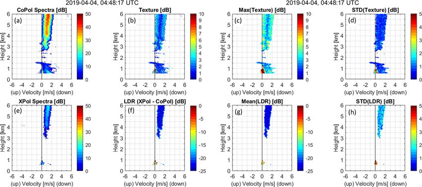
4.2 LDR algorithm branch
This section describes the processing steps of the LDR al-
gorithm (Boxes 5–8 of Fig. 5). In Box 5, an objective noise
threshold nHS (hj ) is estimated from the XPol spectra at each
height (Hildebrand and Sekhon, 1974; Carter et al., 1995).
The XPol spectra with magnitudes greater than nHS (hj )
are defined as signal power (see Eq. 3). Box 6 calculates
the linear depolarization ratio spectra using Eq. (1). The
CoPol and XPol spectra profiles at 04:48:17 UTC from the
precipitation event on 4 April 2019 shown in Fig. 4 are
shown in Fig. 9. The top row of Fig. 9 (Fig. 9a–d) shows
CoPol observations and CoPol texture statistics used in the
CoPol texture algorithm. Figure 9e and f show XPol and
LDR spectra profiles. To estimate regional scattering prop-
erties, the same 5 × 3 velocity–height window used in the
texture algorithm is used to calculate regional LDR statis-
tics throughout the SdB LDR (v , h ) spectra profile (Box 7 of
i j LDR
Fig. 5). Figure 9g and h show the mean SdB (vi , hj ) and
Figure 8. Spectral memberships and binary mask for profile at LDR (v , h ) estimates and suggest that insects are
SD SdB i j
19:19:02 UTC on 31 July 2018. The red color indicates hydrom-
eteor membership and the blue color represents insect membership. present below 1 km with near zero vertical velocity and
(a) Texture algorithm spectral membership. (b) LDR algorithm falling hydrometeors are present above 3 km. The insects are
LDR
spectral membership. (c) Filtered spectral membership. (d) Binary deduced by mean SdB (vi , hj ) between −10 and −5
LDR dB
hydrometeor and insect mask. and the falling hydrometeors by mean SdB (vi , hj ) less
than −20 dB. These inferences are supported by the CoPol
texture
statistics (Fig. 9c and 9d) with insects having large
et al. (2008). One way to improve the classification is to use a max T dB (vi±2 , hj ±1 ) near zero vertical velocities below
threshold that is orthogonal to the observed distributions. The 1 km and smaller values elsewhere. As with the warm shal-
insect and hydrometeor 2D Gaussian functional fits shown in low cumulus cloud event shown in Fig. 6, there are more
Fig. 7b and e have correlation coefficients greater than 0.9 CoPol observations (Fig. 6a–d) than LDR measurements
and indicate the distributions are close to a 1-to-1 slope. After (Fig. 6e–h) below 1.5 km.
creating a line between the hydrometeor and insect distribu- With an objective of separating insect and hydrometeor
tions, an orthogonal threshold can be constructed. Figure 7b scattering regions based on LDR statistics, Fig. 10 shows
and e show the orthogonal threshold developed by analyzing 2D and 1D PDFs of the LDR statistics estimated for all ob-
many hydrometeor and insect observations from 2018 and servations below 1.5 km (to avoid too many hydrometeor
2019 (see Appendix A for details). The analysis presented observations that would prevent any insects from appear-
in Appendix A suggests that the orthogonal threshold has a ing in Fig. 10) for hour 04:00 UTC on 4 April 2019. Fig-
true positive rate of about 90 % for both hydrometeor and ure 10 contains over 1 million LDR statistic samples each
insect scattering observations. Due to the distribution over- calculated over a separate
LDR 5 × 3spectral region. The distri-
lap, a single threshold methodology will not reach a 100 % bution near mean SdB (vi , hj ) = −8 dB is due to insect
LDR (v , h ) =
true positive rate and additional classification or filtering will scattering and the distribution near mean SdB i j
be necessary. One way to improve the classifications due to −20 dB is due
LDR to hydrometeor scattering. A threshold of
distribution overlap or inaccurate thresholds is to apply con- mean SdB threshold
= −15 dB clearly separates the two dis-
tinuity filters to remove random or ephemeral samples due to tributions and is indicated with a dashed line in Fig. 10b,
misclassifications as discussed in Sect. 4.4. Applying the or- which is consistent with estimates from Matrosov (1991) and
thogonal CoPol texture threshold to the example profile from Reinking et al. (1997).
19:19:02 UTC, Fig. 8a shows the insect (blue shading) and Figure 11a and b show the CoPol texture and LDR mem-
hydrometeor (red shading) texture membership classes. Also bership classes for this spectra profile. Blue shading indicates
in Fig. 8 are the LDR insect–hydrometeor classes, the com- insect scattering and red shading indicates hydrometeor scat-
bined classes, and the profile mask, all of which are discussed tering. Note that the texture algorithm identifies both insect
in the next section. and hydrometeor scattering below 1.5 km while the LDR al-
gorithm only detects a few insects at these lower range gates.
Both algorithms identify hydrometeor scattering above about
3 km.
Atmos. Meas. Tech., 14, 4425–4444, 2021 https://doi.org/10.5194/amt-14-4425-2021C. R. Williams et al.: Identifying insects, clouds, and precipitation 4435
Figure 9. Same as Fig. 6 except for the profile at 04:48:17 UTC on 4 April 2019.
Figure 10. Similar to Fig. 7 except for hour 04:00 UTC on
4 April 2019 and for SD(LDR) and mean(LDR) statistics. There Figure 11. Same as Fig. 8 except for the profile at 04:48:17 UTC on
are 1 085 217 samples collected below 1.5 km height. 4 April 2019.
4.3 Combining CoPol texture and LDR algorithm
classifications rithm produced a hydrometeor class when the texture classi-
fication was set to insect class. This logic places more em-
After performing the CoPol texture and LDR algorithms, the phasis on identifying hydrometeors than insects.
binary insect and hydrometeor spectral classifications from One of the physical attributes of hydrometeor scattering
both algorithms are combined and then filtered (e.g., see is that the Doppler velocity spectra span multiple continu-
Figs. 8a, b and 11a, b). Initially, the combined spectral clas- ous velocity bins and over several range gates. Accordingly,
sification is the texture classification because the LDR clas- isolated hydrometeor pixels in the combined spectral classi-
sification will always have fewer valid observations than the fication are removed by requiring at least seven continuous
CoPol observations. To incorporate the LDR classification, hydrometeor pixels in the velocity dimension. All hydrome-
the combined classification is changed only if the LDR algo- teor pixels not satisfying this constraint are set to the insect
https://doi.org/10.5194/amt-14-4425-2021 Atmos. Meas. Tech., 14, 4425–4444, 20214436 C. R. Williams et al.: Identifying insects, clouds, and precipitation
scattering class. The filtered memberships for the two exam-
ple profiles are shown in Fig. 8c for the warm liquid cloud
event on 31 July 2018 and in Fig. 11c for the precipitation
event on 4 April 2019. The red and blue shading corresponds
to hydrometeor and insect scattering classes, respectively.
The final processing step is to reduce the filtered mem-
bership classes into binary masks indicating the presence of
insect or hydrometeor scattering at each range gate (Box 10
of Fig. 5). The insect and hydrometeor masks are set to unity
if that filtered membership class exists for that range gate
hj . In the case when both insect and hydrometeor scatter-
ing are detected at the same range gate, the hydrometeor
mask is set to unity and the insect mask is set to zero. This
logic places more emphasis on identifying robust hydrome-
teor masks and defining masks resulting from either insect
or hydrometeor scattering at each range gate. Figures 8d and
11d show the binary insect and hydrometeor masks for the
two example profiles. Both masks are saved in output data
files and have the variable names insect_mask_raw and hy-
dro_mask_raw (Boxes 11 and 12 of Fig. 5). The suffix raw
designates that these masks were estimated from individual
profiles and without any temporal information from neigh-
boring profiles, which is discussed in Sect. 4.4.
In addition to the binary insect mask, an insect activity in- Figure 12. Measurements and retrievals for hour 19:00 UTC on
dex is generated by counting the number of insect scattering 31 July 2018. (a) CoPol reflectivity (dB). (b) Retrieved hydrome-
teor raw mask (red shading). COGS-derived 6 km × 6 km domain
velocity bins at each height. This insect index Iinsect (hj ) is
average cloud base (red symbols) and cloud top (blue symbols).
defined as (c) Same as panel (b) expect for the retrieved hydrometeor QC1
imax mask. (d) Retrieved insect activity index. The black symbols are
X filtered
ceilometer-derived cloud base.
Iinsect hj = Cinsect vi , h j , (6)
i=1
filtered (v , h ) is the insect spectral classification and
where Cinsect i j
from each spectra profile. These raw hydrometeor masks
has a value of either 0 or 1. This insect index is not an esti- contain random misclassified pixels of hydrometeors below
mate of the insect number concentration because the magni- the ceilometer cloud base height. Most of these false posi-
tude of the insect scattering is not being taken into account. tive hydrometeor mask pixels are removed by sequentially
The authors hypothesize that the insect index should be re- applying two time–height quality control filters.
lated to insect number density, as the breadth of insect ve- The first quality control filter, named QC1 (shown in
locities should increase as the number of insects increases. Fig. 12c), removes temporal outliers by applying a three-
The insect index is available in the output data files with the member temporal continuity filter, which retains all three val-
variable name insect_index_raw. ues if three consecutive values are present. The QC1 filter
also inserts up to three consecutive hydrometeor mask pix-
4.4 Quality control (QC) filtering of the cloud profile els in vertical profiles to fill small gaps in the raw hydrome-
mask teor mask. The second quality control filter, named QC2 (not
shown), applies a low-pass filter to the QC1 filtered mask
Figure 12 shows the time–height cross section of observed by moving a 3 × 3 time–height (approximately 12 s by 90 m)
CoPol KAZR reflectivity (Fig. 12a), the raw hydrome- continuity constraint throughout the domain to robustly iden-
teor mask (Fig. 12b), a time–height filtered hydrometeor tify hydrometeors that are persistent in time and height. Both
mask (Fig. 12c), and the insect index (Fig. 12d) for hour the QC1 and QC2 filtered hydrometeor masks are available
19:00 UTC on 31 July 2018. This is the same event shown in the output data files with variable names hydro_mask_qc1
in Figs. 1 and 2, except with the vertical axis limited to 3 km and hydro_mask_qc2. Figure 12d shows the insect index and
height. The ceilometer cloud base height is shown in each estimates the number of velocity bins in the spectra that con-
panel with black dots. The blue and red plus symbols are tained insect scattering. The color scale is logarithmic with
cloud top and base determined from the COGS stereo cam- a maximum value 256 representing the number of veloc-
era system, which is discussed in more detail in Sect. 5. The ity bins in the spectra. The QC1 hydrometeor mask is plot-
hydrometeor mask in Fig. 12b is the raw mask produced ted for the 4 April 2019 precipitation event in Fig. 4d. The
Atmos. Meas. Tech., 14, 4425–4444, 2021 https://doi.org/10.5194/amt-14-4425-2021C. R. Williams et al.: Identifying insects, clouds, and precipitation 4437
mask identifies the shallow clouds near 1.5 km from about
2–13 min and the precipitating anvil at the beginning of the
hour between 3–4 km that descends to the lowest range gate
just after minute 20. The hydrometeor mask below 1.5 km
that starts at about minute 21 and continues until the end of
the hour except for a shallow gap between minutes 50–55
is due to precipitation at these lower heights, as indicated in
Fig. 11c. There is strong agreement between the ceilometer
cloud base height estimates and the hydrometeor mask before
minute 20. After this time, the hydrometeor mask identifies
raindrops, while the ceilometer identifies cloud base. COGS
measurements are unavailable for comparison purposes dur-
ing this event because COGS is an optical system requiring Figure 13. Difference in the hydrometeor mask QC1 column bot-
daylight. tom and ceilometer cloud base height using 47 d at SGP during
2018 and 2019. There were 12 141 profiles with simultaneous hy-
drometeor mask QC1 and ceilometer cloud bases. (a) 1D PDF of
height difference defined as (hydrometeor mask column bottom)
5 Comparing cloud mask with independent
– (ceilometer cloud base) (m) with 30 m resolution corresponding
measurements to radar range resolution. (b) Colors are 2D distributions of height
difference vs. ceilometer cloud base. Colors represent the percent-
Figures 4 and 12 show significant agreement between age of occurrence relative to the cell with the maximum number
ceilometer cloud base estimates and retrieved QC1 hydrome- of observations. The artifact at negative height differences and low
teor masks. Figure 12 also shows agreement between COGS ceilometer cloud base is due to the radar first range gate at 570 m.
cloud base and top estimates with the QC1 hydrometeor
mask. In comparing the three products, the KAZR hydrom-
eteor masks and ceilometer cloud base estimates appear as base as the hydrometeor mask detects falling raindrops far
discrete cloud events. Conversely, the COGS estimates ap- below the ceilometer detected cloud base.
pear continuous in time, as if COGS is detecting a persistent
cloud layer. This difference is because KAZR and ceilometer
are “soda-straw” observations and COGS is a 6 km × 6 km 6 Conclusions
domain-averaged product produced from three pairs of stereo
cameras positioned around the radar and ceilometer (Romps In addition to detecting cloud particles, vertically pointing
and Öktem, 2018). Figure 12c shows that when the radar and cloud radars are sensitive enough to detect individual insects.
ceilometer both detect clouds, COGS also had a similar cloud If insect contamination is not identified and removed, then
base height estimate. The ceilometer and radar cloud bases radar-derived cloud properties will be incorrect and will not
also showed consistency even at the cloud edges (see near help with validating cloud resolving models or climate sim-
minute 35). Regarding cloud top estimates, COGS estimates ulations. This study used polarimetric radar observations to
are higher than the radar because COGS is a domain average. develop two insect–hydrometeor detection algorithms. The
The Supplement contains images of the QC1 hydrometeor two algorithms use different radar scattering principles to
mask, ceilometer, and COGS retrievals for 47 d correspond- identify small velocity–height regions in the Doppler ve-
ing to 2018 and 2019 LASSO shallow cloud events (LASSO, locity power spectra profile resulting from either insect or
2020). The COGS product is available only for shallow cu- hydrometeor scattering. The results of both algorithms are
muliform clouds and only during daylight hours. combined and then filtered to produce single value insect
Figure 13 compares hydrometeor mask QC1 column bot- and hydrometeor masks at each range gate. The backscat-
toms with ceilometer cloud bases for the 47 LASSO days. tered power from hydrometeors and insects is larger in the
The hydrometeor mask QC1 columns were at least 90 m CoPol channel than the XPol channel, leading to negative
thick (i.e., three consecutive range gates). Using the same LDR values. This difference in sensitivity leads to this study
format as Figs. 7 and 10, Fig. 13b shows the 2D distribution finding that KAZR XPol spectra observations observed fewer
of height differences with the line graph showing 1D PDF. insects than KAZR CoPol observations. This implies that us-
Over 70 % of the 12 141 simultaneous profiles had height ing just a polarimetric signal processing method to identify
differences within ±100 m, which represents ±3 30 m radar insects will not identify all insect clutter affecting CoPol ob-
range gates. There is a small skewness to the height differ- servations and that insect clutter mitigation methods must use
ence PDF (Fig. 13a) that is consistent with the ceilometer CoPol observations to identify all insect clutter in the CoPol
detecting clouds before the radar detects hydrometeors. Also, channel.
during the few precipitation events, the hydrometeor mask One algorithm uses the texture of CoPol Doppler veloc-
bottom was significantly lower than the ceilometer cloud ity power spectra to identify small velocity–height regions of
https://doi.org/10.5194/amt-14-4425-2021 Atmos. Meas. Tech., 14, 4425–4444, 20214438 C. R. Williams et al.: Identifying insects, clouds, and precipitation spectra attributed to insect or hydrometeor scattering. Since The Supplement includes sample images of observed insects are individual point targets, their radar power return KAZR reflectivity, retrieved hydrometeor masks, and veri- is confined to narrow intervals of Doppler velocity and range fication observations from ceilometer and COGS. The pro- gates on the order of 1–3 velocity bins (0.04 to 0.12 m s−1 ) cessing described herein was applied to KAZR observations and 1–3 range gates (30 to 90 m). In contrast, cloud particles for April–October in 2018 and 2019 summer seasons at the and raindrops occur in distributions that extend over many Southern Great Plains (SGP) facility. The insect and hydrom- velocity bins and several range gates, on the order of 5–150 eteor masks for these months are available online in the DOE velocity bins (0.2 to 7 m s−1 ) and 3–150 range gates (90 to ARM archive (Williams, 2021). 4500 m). The CoPol and XPol Doppler velocity power spec- tra from insect scattering have large variability, or texture, while scattering from cloud particles and raindrops produce smoother, less variable spectra. The CoPol texture algorithm uses the texture information to identify small regions of in- sect and hydrometeor scattering. The CoPol texture algo- rithm can be applied to any cloud radar system collecting Doppler velocity power spectra and does not require a cross- polarization channel. The other algorithm uses the linear depolarization ratio (LDR) at each point in the Doppler velocity power spectra to identify regions of scattering due to spherical raindrops, asymmetric ice particles, or asymmetric insects. Unlike pre- vious studies, this work uses the LDR at each spectra bin. After identifying small velocity–height regions of insect and hydrometeor scattering in both algorithms, the spectra clas- sifications are combined and then filtered to account for con- tinuity in the Doppler velocity and vertical range dimen- sions. The filtered spectra classifications are reduced to bi- nary affirmative insect and hydrometeor masks with a sin- gle value at each range gate. An insect activity index is esti- mated at each range gate by counting the number of Doppler velocity spectra bins with insect scattering. Future studies will use insect activity and vertical air motion estimates to explore whether insects are passive tracers or actively pro- pelling themselves through the atmosphere. Often, insects occur at the same height as clouds and during the onset of precipitation. While these are interesting phenomena, the fo- cus of this work is producing robust hydrometeor masks to help identify cloud boundaries, which can be used, for ex- ample, to study the evolution of shallow cumulus clouds in the planetary boundary layer (Gustafson et al., 2017). Us- ing over 12 000 simultaneous ceilometer and radar profiles, it was found that over 70 % of the hydrometeor mask column bottoms were within ±100 m of the ceilometer cloud base (i.e., ±3 30 m radar range gates). The hydrometeor mask col- umn bottom was slightly higher than the ceilometer cloud base. This is to be expected, as the ceilometer detects cloud particles at lower heights than the radar detecting hydrome- teors within the cloud. Atmos. Meas. Tech., 14, 4425–4444, 2021 https://doi.org/10.5194/amt-14-4425-2021
You can also read


