Using Artificial Neural Networks for the Estimation of Subsurface Tidal Currents from High-Frequency Radar Surface Current Measurements - MDPI
←
→
Page content transcription
If your browser does not render page correctly, please read the page content below
remote sensing
Article
Using Artificial Neural Networks for the Estimation of
Subsurface Tidal Currents from High-Frequency Radar
Surface Current Measurements
Max C. Bradbury * and Daniel C. Conley

                                          Coastal Processes Research Group, School of Biological and Marine Sciences, Faculty of Science and Engineering,
                                          University of Plymouth, Plymouth, PL4 8AA, UK; daniel.conley@plymouth.ac.uk
                                          * Correspondence: max.bradbury@plymouth.ac.uk

                                          Abstract: An extensive record of current velocities at all levels in the water column is an indispensable
                                          requirement for a tidal resource assessment and is fully necessary for accurate determination of
                                          available energy throughout the water column as well as estimating likely energy capture for
                                          any particular device. Traditional tidal prediction using the least squares method requires a large
                                          number of harmonic parameters calculated from lengthy acoustic Doppler current profiler (ADCP)
                                          measurements, while long-term in situ ADCPs have the advantage of measuring the real current but
                                          are logistically expensive. This study aims to show how these issues can be overcome with the use of
                                          a neural network to predict current velocities throughout the water column, using surface currents
                                          measured by a high-frequency radar. Various structured neural networks were trained with the aim
                                          of finding the network which could best simulate unseen subsurface current velocities, compared to

                                   ADCP data. This study shows that a recurrent neural network, trained by the Bayesian regularisation
                                          algorithm, produces current velocities highly correlated with measured values: r2 (0.98), mean
Citation: Bradbury, M.C.; Conley,
                                          absolute error (0.05 ms−1 ), and the Nash–Sutcliffe efficiency (0.98). The method demonstrates its high
D.C. Using Artificial Neural
Networks for the Estimation of
                                          prediction ability using only 2 weeks of training data to predict subsurface currents up to 6 months in
Subsurface Tidal Currents from            the future, whilst a constant surface current input is available. The resulting current predictions can
High-Frequency Radar Surface              be used to calculate flow power, with only a 0.4% mean error. The method is shown to be as accurate
Current Measurements. Remote Sens.        as harmonic analysis whilst requiring comparatively few input data and outperforms harmonics by
2021, 13, 3896. https://doi.org/          identifying non-celestial influences; however, the model remains site specific.
10.3390/rs13193896
                                          Keywords: high-frequency radar; neural networks; tidal resource assessment; ocean currents
Academic Editor: Silvia Piedracoba

Received: 18 August 2021
Accepted: 22 September 2021
                                          1. Introduction
Published: 29 September 2021
                                                As the demand for electricity increases globally, with the concurrent commitment of
                                          many countries to lower emission levels, the number of renewable energy developments
Publisher’s Note: MDPI stays neutral
with regard to jurisdictional claims in
                                          is soaring. Tidal stream is likely to play a role in this increase due to the predictability of
published maps and institutional affil-
                                          its power, unlike the other offshore technologies of wind and wave. The kinetic energy
iations.
                                          caused by flood and ebb tides is too low in most areas. However, in some locations, the
                                          combination of tidal factors and local bathymetry can result in velocities that have an
                                          energy potential that is high enough over a large spatial and temporal range in order to
                                          enable production of electricity at a cost-efficient rate, potentially even higher than an
                                          efficient wind site [1]. Currently, tidal energy is a maturing technology with multiple single
Copyright: © 2021 by the authors.
                                          devices deployed and arrays in the planning stages, the most progressed of these being
Licensee MDPI, Basel, Switzerland.
                                          the 398 MW Meygen Tidal Project in Pentland Firth. As high-energy sites are developed,
This article is an open access article
distributed under the terms and
                                          and turbine technology improves to viably produce energy at lower velocities, resource
conditions of the Creative Commons
                                          assessments will need to be conducted for site characterisation of new areas.
Attribution (CC BY) license (https://           The rate of movement and directionality of water are caused by influences from tidal
creativecommons.org/licenses/by/          harmonics, wind, depth, and other factors, each being specific to a site. Site characterisation
4.0/).                                    is important for tidal energy as current speeds are the primary determining factor for

Remote Sens. 2021, 13, 3896. https://doi.org/10.3390/rs13193896                                        https://www.mdpi.com/journal/remotesensing
Remote Sens. 2021, 13, 3896                                                                                             2 of 20

                              power, translating to revenue for a developer. In situ measurements are essential for tidal
                              resource assessment, with additional analysis using modelling or harmonics [2]. ADCPs
                              are useful for point measurement resource assessment, especially for measuring turbulence
                              and local variabilities [3,4]. To increase the spatial coverage, Gooch et al. [5] employed
                              spatial interpolation using ADCP data to display the tidal velocity patterns over an area,
                              with the inclusion of the tidal phase difference. Other research towed an underway ADCP
                              around Pentland Firth at a high pace and resulted in the ability to resolve the vertical
                              velocity profiles of the tidal current including its spatial and temporal anomalies [6], this
                              has a high resource consumption and only provides data for a short period. It was shown in
                              their research that the combination of their in situ results with the constraints of a numerical
                              model could produce an accurate four-dimensional representation of tidal velocity outputs.
                              Evidently, observations from ADCPs do show that they are effective to use, especially
                              in the measurement of turbulence and small-scale variations, and also as validation for
                              hydrodynamic models. However, ultimately, they are disadvantaged by their inability
                              to easily assess the spatial and temporal range required in a resource assessment [7].
                              Alternatively, modelling has proven its potential for current mapping through validation
                              by ADCPs and is now often used for tidal resource assessment [8–10]. However, these
                              require high computational power as well as a lot of detailed data including bathymetry
                              and boundary conditions, which may not be available in many worldwide locations.
                                    Harmonic analysis methods predict the amount of tidal forcing at a point as spectral
                              lines which represent the sum of a set of sinusoids at specific frequencies (cycles per hour).
                              These are obtained as combinations of the totals and differences of integer multiples of
                              six fundamental frequencies, named Doodson Numbers [11], which come about from
                              the motion of celestial bodies [12]. In order to define the amplitude of each frequency,
                              harmonic analysis uses the least squares fit. The amplitude and phase of each frequency
                              characterise a compression of the data in the complete tidal time series. Harmonic analysis
                              is a useful tool for tidal prediction at a point but has a number of drawbacks, namely, the
                              long measurement history required for accurate predictions [13].
                                    The use of shore-based high-frequency (HF) radars for the remote sensing of offshore
                              surface currents and conditions has become increasingly more prevalent [14–16], but has
                              been applied on few occasions for the assessment of subsurface currents. Measurement
                              of surface currents from HF radar works through the transmission of vertically polarised
                              electromagnetic waves which are intercepted and are returned causing an energy spectrum
                              at the receiver. The reflection, when used for ocean currents, is in the form of a Bragg scatter,
                              which results from the reflection of energy by ocean waves with exactly half the wavelength
                              of the transmitted radar waves [17]. Bragg scatter is used because it is the strongest return.
                              The backscatter is returned to the radar carrying information of the surface current velocity
                              and wave spectra. Studies by Thiébaut and Sentchev [18,19] did incorporate a technique
                              using an HF radar, principal component analysis numerical modelling, and a depth power
                              law correlated with ADCP measurements, resulting in a three-dimensional grid of tidal
                              current variability and power density in the water column. It was found that the power
                              available in the bottom layer of their study area was three times lower than near the surface.
                              This is important for the assessment of the optimum hub height of any potential tidal
                              turbine which may be deployed, and the variability of tidal strength allows for design
                              loads for the support structures of devices to be recognised. The HF radar in the study
                              allowed them to apply the technique to the entire area while using real, remotely sensed
                              data rather than modelled, proving the usefulness of the combination of remote sensing
                              with field measurements. New techniques that may increase the ease of assessment are
                              always sought after; an Artificial Neural Network (ANN) could prove a more simple and
                              quicker method than modelling to achieve the same outcome.
                                    ANNs are mathematical models which work similarly to the biological nervous system.
                              ANNs have been extensively used for the prediction of natural processes over the last
                              30 years, including many successful applications within the marine environment [20,21].
                              They have shown their worth in tidal range prediction, instead of harmonic analysis,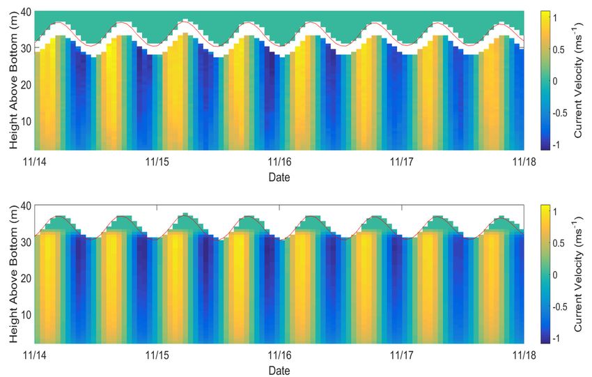
Remote Sens. 2021, 13, 3896                                                                                                            3 of 20

                              demonstrating their ability to predict 30 days of hourly tidal height variation using only
                              a small initial dataset and learning period of one day, in contrast to the length of records
                              required by harmonic analysis [22–26].
                                   For tidal analysis, a recurrent neural network (RNN) architecture is preferable, which
                              are capable of learning features and long-term dependencies from time-series data [27],
                              making it an appropriate choice for the oscillatory nature of the tides to get a sense of
                              where the wave amplitudes are likely to be heading. The defining equation of the RNN is
                              such that given values of the time series, y(t), and the input series, z(t), the model is able
                              to predict new values of y(t) [28].

                                       y ( t ) = f y ( t − 1), y ( t − 2), . . . , y t − n y , z ( t − 1), z ( t − 2), . . . , z ( t − n z )

                                    The n past values are tapped delay lines, storing previous y(t) and z(t) values. The
                              recurrent feature of the network is where these values are regressed onto the new input signal.
                                    The aim of this paper is to assess the capability of a technique combining HF radar
                              surface currents and ANNs for quantification of subsurface currents, to show comparable
                              accuracy to in situ measurements and harmonic analysis, decreasing the resources required
                              for a reliable tidal stream resource assessment of a large area. This will be achieved through
                              the creation of various structured neural networks to find the highest performing network
                              for subsurface current prediction. The ANN will be validated through statistical compari-
                              son to an independent ADCP dataset, and subsequently used for tidal power calculations.
                              The ANN will then be used to associate HF radar surface currents to subsurface currents at
                              another location, followed by discussion of network capabilities and behaviours.

                              2. Materials and Methods
                              2.1. Site and Datasets
                                    The Celtic Sea off the north coast of Cornwall has a high-energy wave regime, suitable
                              for the deployment of wave energy converters. The site is not a potential candidate for a
                              large tidal stream development but is suitable for demonstrating this technique. The tidal
                              movement is predominantly meridional, with a lesser zonal component [29], due to the
                              proximity and morphology of the coast.
                                    Data for the ANN were pre-collected (Conley, 2013, unpublished data), continuously
                              available between March and December 2012.
                                    The surface velocity data used as inputs for the ANN were obtained from a system of
                              two high-frequency Wellen Radar stations positioned 40 km apart at Pendeen and Perran-
                              porth and overlooking the WaveHub test site on the north coast of Cornwall (Figure 1). At
                              each site, there is a 16-element phased-array receiver and a square four-element transmitter
                              orientated parallel to the coast. At Pendeen, the receiver is orientated 113◦ clockwise from
                              true north, hence its boresight is directed 23◦ from north. At Perranporth, the receiver
                              is orientated 35◦ from north with its centroid beam pointed 305◦ N so it aligns with the
                              prevailing westerly swell. The radar stations independently measure the surface current
                              velocity for 17 m 45 s every hour with a range resolution of approximately 1 km and
                              angular resolution of 7◦ . The radars use a “listen before talk” mode [30], which determines
                              the best frequency for transmission within a 250 kHz bandwidth centred on a frequency of
                              12 MHz. This results in transmitted waves being backscattered off ocean waves 12.5 m long
                              at a range of up to 101 km. Surface currents are recordable over the full range while wave
                              products are only available over half the range due to the large signal-to-noise ratio of the
                              second-order returns compared to the first-order echo. The backscattered information is
                              transformed into an orthogonal coordinate system to set it to a 1 km grid [16].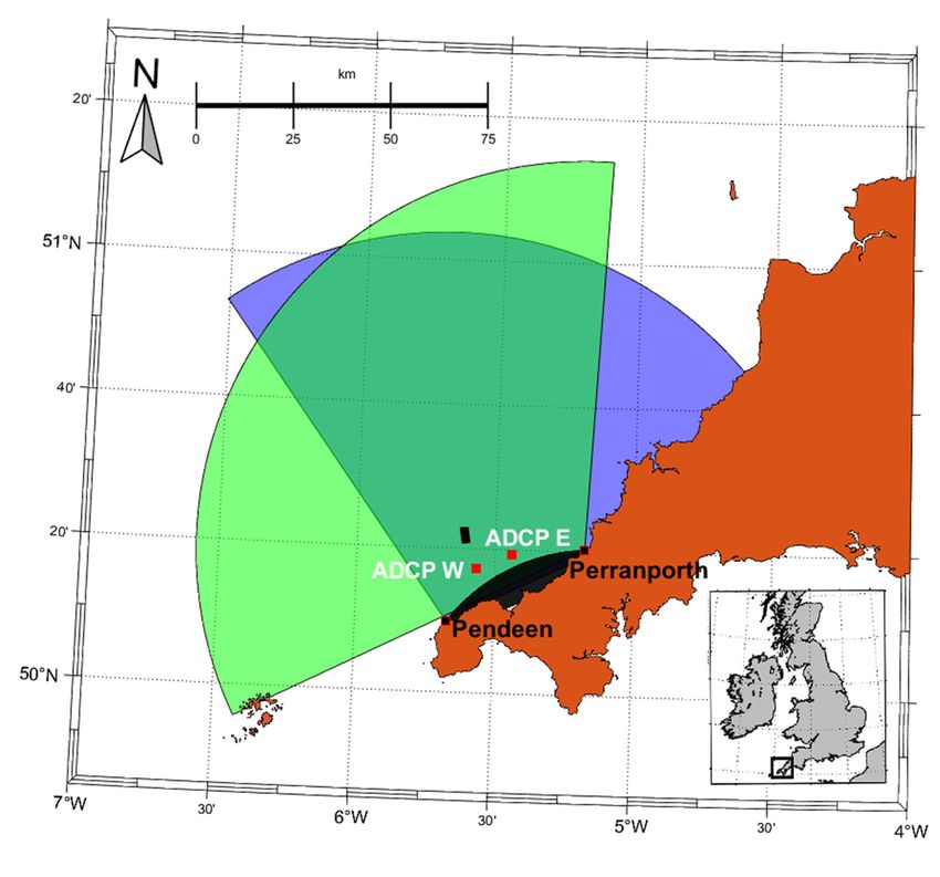
Remote Sens. 2021, 13, x FOR PEER REVIEW 4 of 21
Remote Sens. 2021, 13, 3896 4 of 20
ratio of the second-order returns compared to the first-order echo. The backscattered in-
formation is transformed into an orthogonal coordinate system to set it to a 1 km grid [16].
Figure 1. Map showing the locations of the HF radars at Pendeen and Perranporth and their coverage.
Figure 1. Map showing the locations of the HF radars at Pendeen and Perranporth and their cover-
The red squares represent ADCP west and east. The rectangle represents the WaveHub test site.
age. The red squares represent ADCP west and east. The rectangle represents the WaveHub test
site.
Two upward-looking Teledyne RD WorkHorse ADCPs were deployed to collect
subsurface velocity data to train and validate the ANN. ADCP-West was placed 16 km
Two upward-looking Teledyne RD WorkHorse ADCPs were deployed to collect sub-
from Pendeen and 29 km from Perranporth, deployed at a mean depth of 34 m, while
surface velocity data to train and validate the ANN. ADCP-West was placed 16 km from
ADCP-East was located 24 km from Pendeen and 19 km from Perranporth deployed at
Pendeen and 29ofkm
a mean depth 37 from Perranporth,
m, with deployed
a separation at a mean depth
of approximately 10 kmof 34 m, while
between ADCP-
the two. The
East
ADCPs operate at 600 kHz in the Janus configuration with four beams located 20◦mean
was located 24 km from Pendeen and 19 km from Perranporth deployed at a from
depth of 37
vertical. m, with
Current a separation
velocities of approximately
were measured 10 intervals
at bin depth km between themtwo.
of 0.75 every The
10 ADCPs
minutes
operate at 600 kHz in the Janus configuration with four beams located 20°
at 2 Hz, with the first bin being 1.86 m above the seabed. At 600 kHz, the accuracy from vertical.
of the
Current
sensor isvelocities wereADCPs
±0.3%. The measuredwereatperiodically
bin depth intervals
recoveredof 0.75 m every
for data 10 minutes
retrieval at 2
and battery
Hz, with the first
replacement, binredeployed
then being 1.86 as
m above the
close to seabed.
the At 600
previous kHz, as
location thepossible.
accuracy of the sensor
is ±0.3%. The ADCPs were periodically recovered for data retrieval and battery replace-
ment, then redeployed
2.2. Metrics as close
Used in Neural to the previous location as possible.
Network
The metrics used as inputs to the ANN in this paper must be covered by the radar or
2.2. Metrics
be from Used in
readily Neural Network
available data to maintain the advantage of this method over traditional
The metrics
methods. used as
This means inputs
that whiletodensity
the ANN in this paper
differences must factors
and other be covered
mayby thehad
have radar or
some
be from readily
influence on theavailable
subsurfacedata to maintain
currents, they the
were advantage
excluded.ofThe
thismetrics
method over
used astraditional
inputs are:
methods. This
the surface meansabove
velocity that while
where density differences
the subsurface and other
current wasfactors may havealong
to be predicted, had some
with
the surrounding
influence four surface
on the subsurface velocities
currents, and
they the tide
were varying
excluded. depth.
The metricsTheused
surrounding
as inputseight
are:
velocities
the surfacewere also above
velocity trialled. However,
where the network
the subsurface had lower
current performance.
was to be predicted,Wind velocity
along with
andsurrounding
the wave field four
datasurface
could have beenand
velocities obtained
the tideand applied
varying to the
depth. Thenetwork. However,
surrounding eight
Lu and Lueck
velocities found
were also that 91%
trialled. of the the
However, subsurface
network flow velocity
had lower in their testWind
performance. site could be
velocity
attributed to the lunar- and solar-influenced tides [31], showing these additional
and wave field data could have been obtained and applied to the network. However, Lu methods
would be of small importance while adding extra neurons and training time to the network.
Additionally, the network performed sufficiently well without these inputs, so they were
not added to reduce network complexity. This ANN technique combined with the radar
has a huge advantage over an ANN alone, the constant radar input means that errors will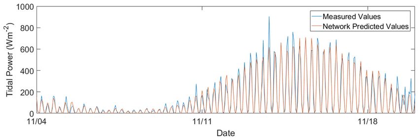
Remote Sens. 2021, 13, 3896                                                                                           5 of 20

                              increase less over time, whereas an ANN alone would soon begin predicting off its own
                              predictions and reduce in accuracy over time.
                                   Both the data processing and ANN creation were carried out in MathWorks’ Matlab
                              and the Matlab Neural Network Toolbox.
                                   The surface velocities above the ADCP which were to be used as inputs to the ANN
                              were identified using the average coordinates of the ADCP placement locations. Surface
                              velocity time series were made at these locations. Two linear interpolations were applied
                              to the data; first of all, the HF radars occasionally failed to record if the data received
                              from a particular cell were below a quality threshold, these were interpolated using their
                              surrounding time points to provide continuous data. Secondly, due to the difference in
                              sampling rates and times of the two instruments, the ADCP data, which collected data
                              more frequently, was linearly interpolated over the times at which the surface velocities
                              were collected, producing surface, subsurface velocity (both east and west components),
                              depth and time data with 6825 hourly time points spanning the same period. The upper
                              10% of the water column was removed from the ADCP data as this near-boundary region
                              is subject to sidelobe interference [32]. The radar data were then arranged into a format
                              which the ANN would take as an input, while the ADCP data would be the output.

                              2.3. Neural Network Creation and Analysis
                                    The architecture of the RNN in this work consists of 6 input neurons, equivalent to the
                              five radar surface velocities surrounding the ADCP and one depth predictor. The predicted
                              velocity at 52 depth bins is represented by the network output, thus, there are 52 neurons
                              in the output layer. The learning ability of an ANN is dependent on the architecture. If
                              the network is too small (too few hidden neurons), it may not have a large enough degree
                              of freedom to learn the relationships between the data. Whereas, if the number of hidden
                              neurons is too large, it can bring about overfitting, where the network fails to generalise
                              with new datasets. The number of hidden neurons was varied (1–50), and the highest
                              performing was chosen, based on statistical tests explained further down this section,
                              comparing unseen data and the network’s predictions.
                                    Several training functions were also employed to obtain a network with the highest
                              performance and generalisation to new data. These training methods were, the gradi-
                              ent descent method with adaptive learning rate (GDA), the scaled conjugate gradient
                              method (SCG), the Levenberg–Marquardt algorithm (LM), and the Bayesian regularisation
                              backpropagation method (BR), which is based on LM.
                                    In formulating the network, available data for 2 weeks were used, representing an
                              entire tidal cycle, making 336 hourly time points (6–19 June 2012). Data for more than
                              2 weeks were also used for training (4 and 8 weeks), but there was no improvement in
                              performance. Performance began to deteriorate once data for 1 week were used. These
                              training data were further split into 70% for training, 15% for model validation, and 15%
                              for testing. The data were divided sequentially, rather than randomly, in order to enable the
                              feedback delays in the recurrent to learn relationships between neighbouring data points.
                              This left any of the remaining 6151 time points for manual testing to assess the capability of
                              the ANN on predicting unseen data. The model was trained by the reduction in the mean
                              square error (MSE) criterion to evaluate performance during training.
                                    Since the performance of a network varies between each training session with the same
                              inputs, due to its ability to find different solutions to problems, each network was required
                              to be trained multiple times in order to obtain a high-performing network. Following the
                              calculations of Iyer and Rhinehart [33], the networks should be trained 90 times each to be
                              99% confident that the best version trained was within the best 5% of possible networks.
                              Through undertaking network training in a loop, starting with random initial weights
                              each time, the 4 training functions, along with trialling 1 to 50 hidden neurons, trained
                              90 times each resulted in 18,000 networks being trained. These were assessed using the
                              statistical tests below. Tapped delay lines were placed connecting the output of the first
                              to fourth hidden neurons back to the input of the first neuron to let the network have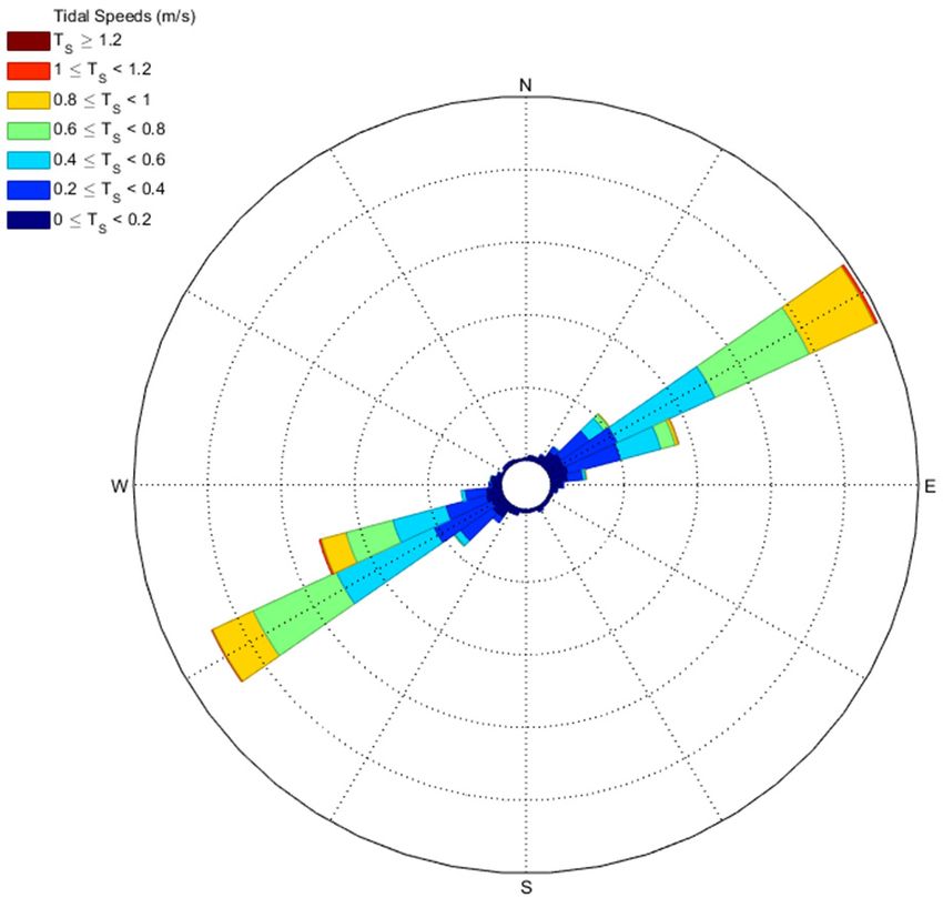
Remote Sens. 2021, 13, 3896                                                                                                             6 of 20

                                      memory of the previous four timesteps to predict the next. This number of lines produced
                                      the highest performing networks; when there were less than four hidden neurons, delay
                                      lines were present on all hidden neurons. Once trained sufficiently, the network was used
                                      to predict velocities at any height above the seabed, at any time in the available data, and
                                      subsequently used to produce products necessary for tidal resource assessment [2]. In
                                      addition, the networks were used to predict subsurface currents at the location of ADCP-E,
                                      10 km from where the network was trained.
                                           Statistical tests were used to assess the network’s performance on unseen data. It is
                                      imperative to use multiple statistical tests as single tests such as the coefficient of correlation
                                      might show good correlation for consistent errors. The tests used were: coefficient of
                                      correlation (r), coefficient of determination (r2 ), root mean square error (RMSE), mean error
                                      (ME) (to show prediction bias), mean absolute error (MAE), mean absolute percentage error
                                      (MAPE), and the Nash–Sutcliffe hydrological efficiency (used to assess the predictive power
                                      of hydrological models where the output ranges from −∞ to 1, and where E = 1 would be
                                      a perfect match) [34].

                                      3. Results
                                      3.1. Performance of Neural Network Structures
                                            The independent data on which the network was tested were for 110 days spanning
                                      from August to December. The best-performing network size of each training function
                                      from the 18,000 created is shown in Table 1, for the east velocity component, along with
                                      statistical differences between the network predicted time series and the unseen measured
                                      time series. Training speed was between 15 seconds and 2 minutes for all GDA and SCG
                                      network sizes, while LM and BR began at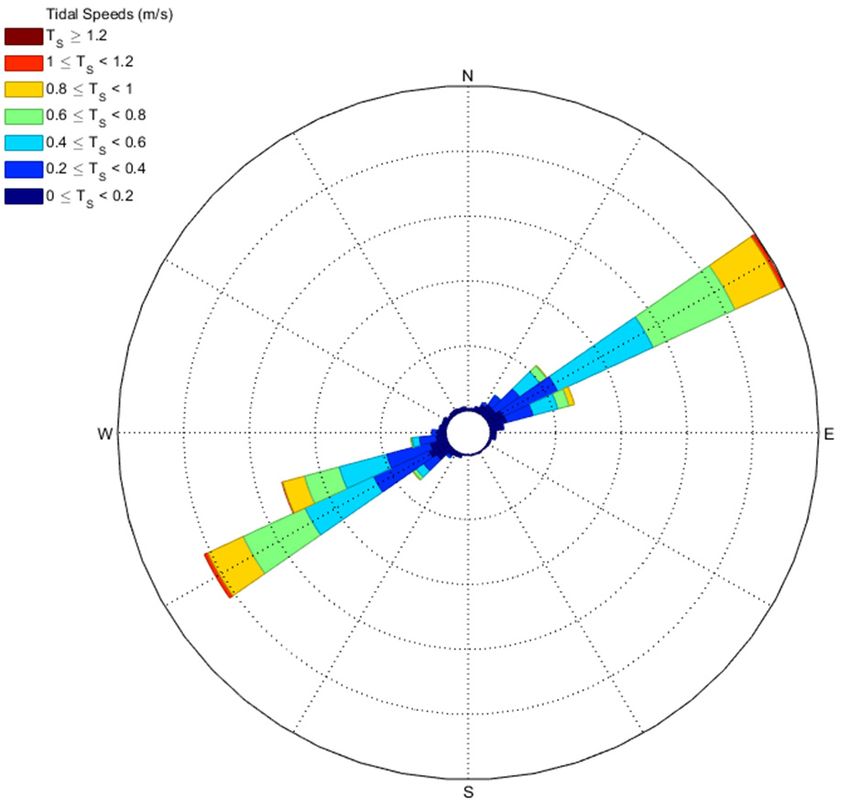
Network Hidden RMSE ME
r r2 STD (ms−1) MAE (ms−1) MAPE (%) E
Function Layers (ms−1) (ms−1)
GDA 22 0.961 0.924 0.247 0.127 −0.018 0.059 N/A 0.917
SCG 27 0.975 0.951 0.251 0.050 −0.008 0.046 N/A 0.949
Remote Sens. 2021, 13, 3896 7 of 20
LM 1 0.982 0.964 0.263 0.043 −0.008 0.039 N/A 0.963
BR 1 0.979 0.958 0.239 0.050 −0.005 0.0037 N/A 0.958
The
Thescatter
scatterplot
plotininFigure
Figure2,2,showing
showingpredicted
predictedvs.
vs.measured
measuredvelocities
velocitiesover
overthe
thetime
time
series
seriesusing
usingthe
thebest
bestBRBR network,
network,shows
showsthat thethe
that network cancan
network reliably predict
reliably tidaltidal
predict velocities
veloc-
from
ities the
fromshort training
the short dataset
training (2 weeks).
dataset (2 weeks).
Figure2.2.Scatterplot
Figure Scatterplotofofthe
themeasured
measured vs.
vs. predicted
predicted east
east velocities
velocities at
at 20
20 m
m above
above the
the seabed
seabed by
by BR,
BR,
around the exact fit line.
around the exact fit line.
3.2.
3.2.Vertical
VerticalVelocity
VelocityProfile
Profile
Knowledge
Knowledgeofofthe vertical
the variation
vertical in current
variation velocity
in current is a critical
velocity step instep
is a critical tidalinresource
tidal re-
assessment and wasand
source assessment alsowas
important in this work
also important to work
in this confirm BR as theBR
to confirm highest
as the performing
highest per-
network.
forming While
network.it seemed
While it the GDA and
seemed the SCG
GDAfunctions
and SCGwere capable
functions of accurate
were capable prediction
of accurate
of current time series at select depths, upon averaging the vertical current
prediction of current time series at select depths, upon averaging the vertical current profile pro-
on
16 spring flood tides, these methods predicted a large net underprediction.
file on 16 spring flood tides, these methods predicted a large net underprediction. Through
visual
Throughassessment and by using
visual assessment and rbyand ME,r and
using the BR
ME,function producesproduces
the BR function the profile thewhich
profile
best
whichrepresents the real measured
best represents profile (Figure
the real measured profile3,(Figure
Table 3). The depth-averaged
3, Table velocity
3). The depth-averaged
predicted by the network was 0.833was −1 , compared to 0.824 ms−1 measured. r and ME
ms0.833
Remote Sens. 2021, 13, x FOR PEER REVIEW predicted
velocity by the network ms−1, compared to 0.824 ms−1 measured. 8 of 21 r and
could not be calculated above 29 m where the ADCP data had
ME could not be calculated above 29 m where the ADCP data had been removed. been removed.
(a) (b)
3. (a) 3.
FigureFigure Current velocity
(a) Current profile
velocity using
profile the
using theBR
BRtraining
training function. (b)Current
function. (b) Current velocity
velocity profile
profile using
using the GDA
the GDA function.
function.
Blue: measured
Blue: measured values,
values, orange:
orange: network
network prediction,and
prediction, and black:
black: mean
meanwater
waterlevel.
level.
Table 3. r and ME of the different trained functions on the predictions of vertical velocity profiles.
Function GDA SCG LM BR
r 0.925 0.989 0.996 0.997
ME −0.0519 −0.0170 0.0155 0.0087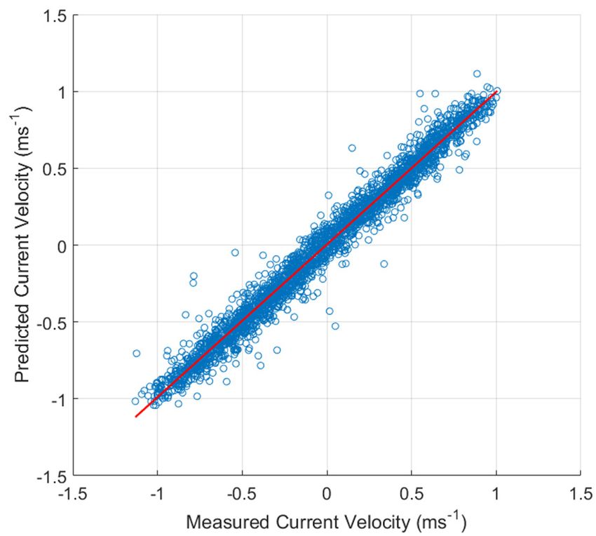
Remote Sens. 2021, 13, 3896 8 of 20
Table 3. r and ME of the different trained functions on the predictions of vertical velocity profiles.
Function GDA SCG LM BR
r 0.925 0.989 0.996 0.997
ME −0.0519 −0.0170 0.0155 0.0087
BR was also the best training function for the north current profile. These networks
were used from henceforth.
3.3. Time Series Prediction
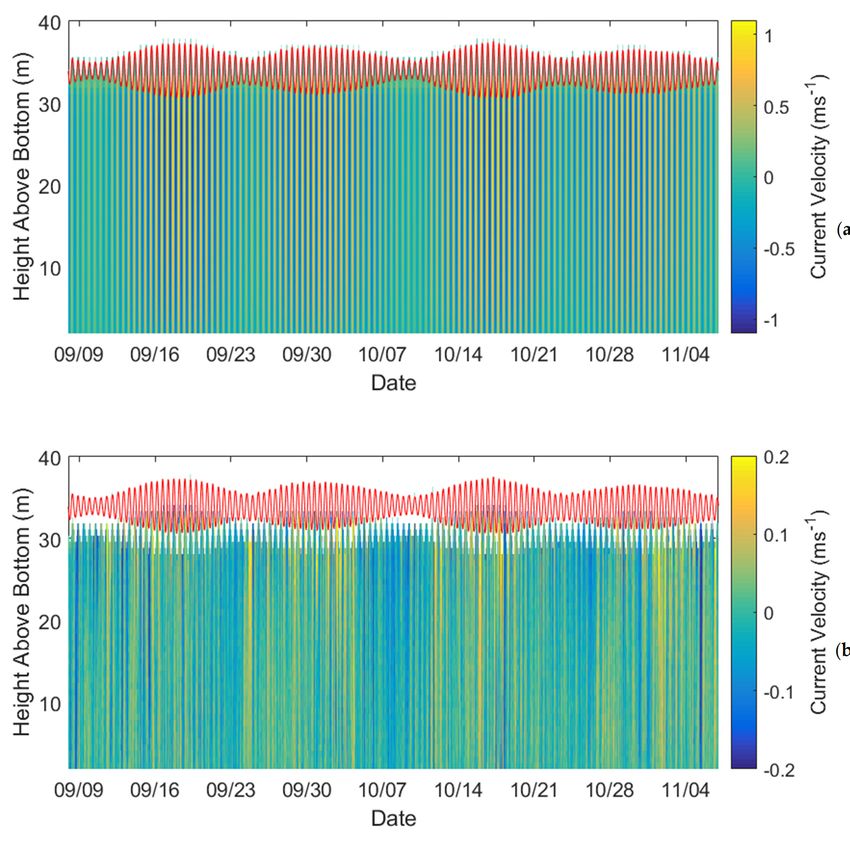
Figures 4 and 5 illustrate how the network was able to predict the E-W velocities at all
depths of the water column, showing the diminishing velocities toward the seabed, using
only surface velocities. The error in prediction shown in Figure 4b is mostly contained
Remote Sens. 2021, 13, x FORbelow ±0.05 other than a few exceptions. The measured and predicted velocities9 are
PEER REVIEW of 21 in
phase and the fortnightly cycle is reproduced.
(a)
(b)
Figure 4. (a) Plot4.of(a)the
Figure predicted
Plot currentcurrent
of the predicted velocity throughout
velocity the water
throughout column.
the water column.(b)(b)Error
Errorbetween
between the predictionsand
the predictions and
measured measured
data. Reddata. lineRed
= water
line =depth. Top 10%
water depth. Topis white
10% despite
is white the the
despite ANNs
ANNsprediction
predictionasasthe
thedata
data were removedininthe
were removed the
ADCP comparison
ADCP comparison due to sidelobe
due to sidelobe interference.
interference.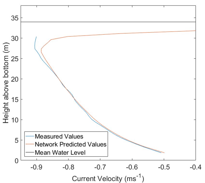
Remote Sens. 2021, 13, 3896                                                                                                       9 of 20
Remote Sens. 2021, 13, x FOR PEER REVIEW                                                                                       10 of 21

                                                                                                                               (a)

                                                                                                                               (b)

     Figure 5. (a)5.Enhanced
        Figure               comparison
                      (a) Enhanced        of measured
                                    comparison           velocity variation.
                                                   of measured               (b) Network(b)
                                                                   velocity variation.   predicted velocity
                                                                                             Network        variation.
                                                                                                      predicted        Red variation.
                                                                                                                 velocity  line =
     water depth.   White space below red line is the location of the inaccurate ADCP  data.
        Red line = water depth. White space below red line is the location of the inaccurate ADCP data.

                                        TheThe
                                            predictions  for the
                                                predictions    fornorth component
                                                                   the north        network
                                                                              component      also showed
                                                                                          network         good agreement,
                                                                                                   also showed            alt-
                                                                                                                 good agreement,
                                 hough    the error figure  contained  more  instances of blue, showing a general underpredic-
                                     although the error figure contained more instances of blue, showing a general underpredic-
                                 tion,tion,
                                        more  so at
                                            more  soneap  tides.
                                                     at neap  tides.

                                 3.4.3.4.
                                     TotalTotal Velocity
                                            Velocity  andand  Direction
                                                          Direction
                                           Figure
                                      Figure       6 shows
                                                6 shows   the the current
                                                               current  roserose generated
                                                                              generated     from
                                                                                         from      measured
                                                                                               measured   andand network
                                                                                                              network     predicted
                                                                                                                       predicted
                                     values, once   the  northern and  eastern  current velocities had been combined,
                                 values, once the northern and eastern current velocities had been combined, showing  showing  good
                                     predictability   of the network.
                                 good predictability of the network.
                                      3.5. Tidal Power
                                (a)                                                          (b)
                                           The tidal power was calculated using the combined velocities. The impact of the
                                      incident current angle on the power take-off of a non-yawing bi-directional turbine was
                                      calculated by adding the cosine response. Table 4 shows the measured mean raw power
                                      before the angle was considered, followed by the measured power considering the angle,
                                      and then each network predicted power considering the angle, showing again that BR
                                      predicted the best network, closely followed by LM.
                                           Figure 7 shows a short period of measured, and network predicted powers. The
                                      network appeared to underpredict some of the largest, abnormal peaks but overpredicted
                                      the medium-sized peaks. This pattern of predictions resulted in a mean power difference of
                                      only 0.51 Wm−2 over the 3.5 months. The inclusion of the cosine response showed that the
                                      tides have a very high angular fidelity, showing only 0.58 Wm−2 decrease in power. The
                                      power–frequency plot (Figure 8) shows high similarity between network and measured
                                      values, showing that using the network predicted or measured values may have little
                                      impact on power prediction.

                          Figure 6. (a) ADCP measured current rose. (b) Network predicted current rose.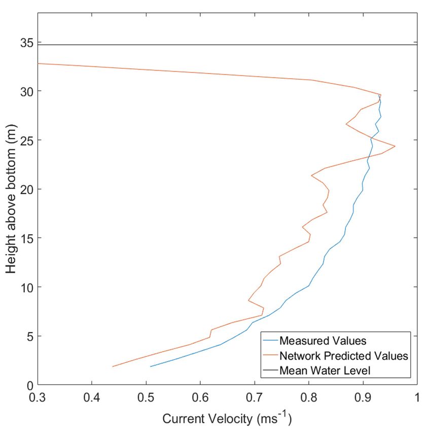
hough the error figure contained more instances of blue, showing a general underpredic-
tion, more so at neap tides.
3.4. Total Velocity and Direction
Remote Sens. 2021, 13, 3896 10 of 20
Figure 6 shows the current rose generated from measured and network predicted
values, once the northern and eastern current velocities had been combined, showing
Remote Sens. 2021, 13, x FOR PEER REVIEW 11 of 21
good predictability of the network.
(a) (b)
3.5. Tidal Power
The tidal power was calculated using the combined velocities. The impact of the in-
cident current angle on the power take-off of a non-yawing bi-directional turbine was cal-
culated by adding the cosine response. Table 4 shows the measured mean raw power be-
fore the angle was considered, followed by the measured power considering the angle,
and then each network predicted power considering the angle, showing again that BR
predicted the best network, closely followed by LM.
Table 4. Measured mean power before accounting for the angle of current (raw power), consider-
ing incident angle (measured), and each training method’s best-performing networks prediction of
mean power and error.
Network Percentage
Mean Power (Wm ) Error from Mean
−2 Max Power (Wm−2)
Measured (%)
Raw power 127.72 - 904.95
Measured 127.14 - 904.82
GDA 124.03 −2.48 928.03
Figure6.6.(a)
Figure (a)ADCP
ADCPmeasured
measuredcurrent
currentrose.
rose.(b)
(b)Network
Networkpredicted
predictedcurrent
currentrose.
rose.
SCG 126.17 −0.77 777.68
LM 128.10 0.75
Table 4. Measured mean power before accounting for the angle of current (raw power), considering incident 931.42
angle
(measured), and each training method’s BR 126.63
best-performing networks −0.40 and error.
prediction of mean power 875.88
Figure 7 shows a−short Network
period Percentage
of measured, andError
network predicted powers.
Mean Power (Wm 2) Max Power (Wm−The
2 ) net-
work appeared to underpredict fromsomeMean Measured
of the largest,(%)
abnormal peaks but overpredicted
Raw power the medium-sized
127.72 peaks. This pattern of predictions
- resulted in a mean904.95
power difference
Measured 127.14 - 904.82
of only 0.51 Wm over the 3.5 months. The inclusion of the cosine response showed that
−2
GDA 124.03
the tides have −2.48
a very high angular fidelity, 928.03 in power.
showing only 0.58 Wm−2 decrease
SCG 126.17 −0.77 777.68
LM
The power–frequency
128.10
plot (Figure 8) shows0.75
high similarity between network
931.42
and meas-
BR ured values,126.63
showing that using the network predicted
−0.40 or measured values
875.88 have little
may
impact on power prediction.
Figure 7. Extract of
of time
time series
series of
ofmeasured
measuredand
andpredicted
predictedcurrent
currentpower.
power.Blue:
Blue:measured
measuredvalues,
values,
and orange: network prediction.Remote Sens. 2021, 13, 3896 11 of 20
Remote Sens. 2021, 13, x FOR PEER REVIEW 12 of 21
Figure 8.
Figure 8. ADCP
ADCPmeasured
measuredand
andneural
neural network
network predicted
predicted frequency
frequency of tidal
of tidal power
power occurrence
occurrence separated
separated into
into 50 Wm 50−2Wm −2
bins.
bins. Blue: measured values, and orange: network prediction.
Blue: measured values, and orange: network prediction.
3.6. Application to Other Areas
3.6. Application to Other Areas
Using the trained network to predict nearby subsurface currents would be a pinnacle
Using the trained network to predict nearby subsurface currents would be a pinnacle
finding to reduce the resources required for a resource assessment. The current velocities
finding to reduce the resources required for a resource assessment. The current velocities
at the east ADCP were consistently slower than at the training location. Using the same
at the east ADCP were consistently slower than at the training location. Using the same
network
network as as the
the previous
previous sections,
sections, the
the network
network consistently
consistently overestimated
overestimated peak peak velocities.
velocities.
Despite the mean absolute velocity difference between the measured
Despite the mean absolute velocity difference between the measured and predictions and predictions be-
ing
beingonly
only0.03 m sm,sthis
0.03
−1 translated
−1 , this to a large
translated difference
to a large in theinresulting
difference meanmean
the resulting power; 29.73
power;
Wm −2 measured and 41.25 Wm−2 predicted.
− 2
29.73 Wm measured and 41.25 Wm predicted. − 2
To achievebetter
To achieve betterpredictions
predictionsatatADCP-E,
ADCP-E,withwitha anetwork
network trained
trained atat ADCP-W,
ADCP-W, a num-
a number
ber of network modifications were made. Firstly, the SCG network
of network modifications were made. Firstly, the SCG network with the optimum 27 hidden with the optimum 27
hidden neurons produced the most accurate predictions, along
neurons produced the most accurate predictions, along with increasing the number of with increasing the num-
ber
delayof lines
delaytolines to 12. Finally,
12. Finally, removing removing
the depth the
asdepth as input improved
input improved predictions predictions
at ADCP-E, at
ADCP-E,
due to thedue to the different
different bathymetry. bathymetry.
Training Training
of the ANN of the ANN
using using
the samethe same of
period period
data of
it
data it was to be tested on also improves predictions, i.e., when trained
was to be tested on also improves predictions, i.e., when trained using August-October at using August-
October atitADCP-W,
ADCP-W, could betterit could
predict better predict thecurrents
the subsurface subsurface 10 km currents 10 km
east over the east
sameover the
period.
same period. This greatly lessened the consistent overprediction, reducing
This greatly lessened the consistent overprediction, reducing the mean current difference the mean cur-
rent
to 0.016 m s−1 and
difference to 0.016 m s−1 and
reducing meanreducing mean power
power difference Wm−2 to
difference
to 4.8 Wm−2−(36.83
4.8 Wm
(36.83 Wm−2
2 measured
measured
and 41.59 Wm − 2
and 41.59 Wm predicted),
predicted),−2
peaks were peaks
alsowere also suppressed,
suppressed, although although
still higher still higher
than the
than the ADCP-W
ADCP-W predictions, predictions,
shown byshown the farby the far
higher higher
MAPE MAPE
(Table 5).(Table 5).
Table 5. 5.
Table Statistics ofof
Statistics the ADCP-E
the prediction
ADCP-E byby
prediction SCG network.
SCG network.
Network Hidden Network Hidden STD RMSE ME MAE MAPE
r r2 STD (ms−1 ) r
RMSE (msr2−1 ) ME (ms−1 ) MAE (ms−1 ) MAPE (%) EE
Function Layers Function Layers (ms−1) (ms−1) (ms−1) (ms−1) (%)
SCG 27 0.976 SCG 0.37727
0.953 0.976 0.079
0.953 0.377
−0.0130.079 −0.013
0.054 0.054 10.68
10.68 0.941
0.941
Comparison of the mean spring flood velocity profiles in Figure 9 shows that at
Comparison of the mean spring flood velocity profiles in Figure 9 shows that at
ADCP-E, there is a large overprediction bias in all but the lowest 6 m of the water column.
ADCP-E, there is a large overprediction bias in all but the lowest 6 m of the water col-
The largest error being 0.1 ms−1 (14.60% error). The network similarly overpredicts veloc-
umn. The largest error being 0.1 ms−1 (14.60% error). The network similarly overpredicts
ities during ebb, contributing to the overall negative mean error of the network.
velocities during ebb, contributing to the overall negative mean error of the network.Remote Sens.
Remote 2021,
Sens. 13,13,
2021, 3896
x FOR PEER REVIEW 1213
of of
2021
Figure
Figure 9. 9.Velocity
Velocity profile
profile at ADCP-E,
at ADCP-E, trained
trained by SCG
by SCG method
method using
using ADCP-W.
ADCP-W. Blue:Blue: measured
measured values,
values,
and andnetwork
orange: orange: prediction.
network prediction.
4.4.Discussion
Discussion
4.1.
4.1.Neural
NeuralNetwork
NetworkPerformance
Performanceand andBehavior-ADCP-W
Behavior-ADCP-W
4.1.1. Current Velocity Time Series
4.1.1. Current Velocity Time Series
Despite all training functions being able to adequately predict both the pattern and
Despite all training functions being able to adequately predict both the pattern and
magnitude of the tidal velocities, it was imperative to choose the best-performing network
magnitude of the tidal velocities, it was imperative to choose the best-performing network
as cubing the velocity for power would enhance inaccuracies. The RMSE values ranged
as cubing the velocity for power would enhance inaccuracies. The RMSE values ranged
from between 13–16% of their corresponding STDs while the Nash–Sutcliffe Efficiency was
from between 13–16% of their corresponding STDs while the Nash–Sutcliffe Efficiency
always over 90%, suggesting high prediction efficiency [35]. While the difference in errors
was always over 90%, suggesting high prediction efficiency [35]. While the difference in
is minimal between training function outputs due to all functions accurately predicting
errors is minimal between training function outputs due to all functions accurately pre-
the majority of the tidal cycle, the small difference in error was caused by the network’s
dicting the majority of the tidal cycle, the small difference in error was caused by the net-
differing abilities to predict peak currents. The GDA function was the most variable, often
work’s differingduring
underestimating abilitiesspring
to predict peak
tides, currents.by
sometimes The0.1GDA
ms−function
1 at peakwas the most
ebbing tide.varia-
As
ble, often underestimating during spring tides, sometimes by
found previously in a wide variety of problems, the LM functions, including BR, which 0.1 ms −1 at peak ebbing tide.
isAs found
based onpreviously
LM, outperformin a widethevariety
simpleofgradient
problems, the LM
descent andfunctions, including gradient
scaled conjugate BR, which
methods [36–39]. Based upon r and MAPE values of the BR network (0.99 and gradient
is based on LM, outperform the simple gradient descent and scaled conjugate 4.63%,
methods [36–39].
respectively), Basedcan
this model upon r and MAPE
be described as avalues of the BRfor
good predictor network (0.99 and[40].
tidal modelling 4.63%,There-
spectively), this model can be described as a good predictor
high-quality statistics of the BR network in comparison to the measurements show that for tidal modelling [40]. The
high-quality statistics of the BR network in comparison to the
the HF radar-ANN technique proves a useful tool for analysis of subsurface current time measurements show that
the HF
series overradar-ANN
any periodtechnique proves
at the training a useful tool for analysis of subsurface current time
location.
series
Theover
majorany period atofthe
limitation thetraining
ANN islocation.
that it is a black box model, failing to simulate the
internal The major limitation
physical processes of of the ANN
a tidal is thatThe
system. it issimulation
a black boxof model,
this isfailing
of vitaltoimportance
simulate the
internal
for resource physical processes
assessments. of a tidalbecause
In addition, system. theTheblacksimulation
box model of this is of
does notvital importance
allow insight
for resource assessments. In addition, because the black box model
into the calculations made to reach the target, assumptions of hydrodynamics which caused does not allow insight
into the calculations
network behaviours are made. made to reach the target, assumptions of hydrodynamics which
caused network
Analysis behaviours
of the colour plots are(Figures
made. 4 and 5) shows that the network generally has a
positive Analysis of thespring
bias around colourtide,
plotsand(Figures 4 and
negative 5) shows
around neap that
tide.theTo network
determine generally has a
the cause,
a positive
networkbias wasaround
trainedspring
over a tide, and negative
different period toaround
identifyneap tide. To
if unique determine
conditions the cause,
during the
a network
initial was trained
two weeks over a different
caused errors. There wasperiod to identify
no significant if unique
difference conditions
in errors to theduring
originalthe
initial two
training weeks
period. Thecaused
errorerrors.
must, There was no
therefore, be significant
in the network’sdifference in errorsof
application toweights
the origi-
nalcalculations.
and training period. The error must, therefore, be in the network’s application of weights
andAlong
calculations.
with the above small-magnitude long-period bias, some short but pronounced
errors Along
also exist.
withWhere theysmall-magnitude
the above occur, they are present
long-periodthroughout
bias, some the entire water
short but column,
pronounced
identifiable
errors alsoas distinct
exist. Where bars, a different
they colour
occur, they areto their surroundings.
present throughout the The network
entire waterpredicts
column,
the time series
identifiable as of each bars,
distinct deptha bin independently
different colour to their [41],surroundings.
not considering Thethe relationship
network predictsRemote Sens. 2021, 13, 3896 13 of 20
between the present bin and those above and below. Therefore, as the network learns
the recurring features of each depth time series, it is unlikely to make the same error
independently at each bin. The resulting implication is that errors between predictions and
the measured values are caused by abnormal surface currents during training, causing the
network to predict accordingly, or abnormal ADCP measurements in the testing data.
Several behaviours of the network were noted throughout the analysis. The network
attempted to predict the upper 10% of the water column (Figures 4a and 5b), even though
the data were removed from its training data. It is impossible to confirm if the network’s
predictions for this region are correct. However, some suspicions may be discussed. The
upper 10% looks to be well predicted at low tides due to the continuation of the lower
currents to the surface, whereas at high tide, the velocities unrealistically approach 0 ms−1 .
It appears the network tries to draw from any values in a depth bin, so as the low waters
are more often submerged and below the 10% threshold, there is more for the ANN to learn
from. At depth bins always in air or the threshold, the network can only predict 0 ms−1 ,
and heights which are mostly in the upper 10% are inaccurate due to limited data.
4.1.2. Velocity Profiles
In the prediction of the velocity profiles, the alike functions behaved similarly, BR and
LM net-overpredicted while GDA and SCG underpredicted. The BR function predicted
the closest fit to measured values (99.69%), as well as the most natural-looking decrease in
velocity with depth. The GDA method produced the lowest correlation (92.49%) with a
much more sporadic pattern than other methods. This is likely because the appropriate
learning rate could not be found, despite running numerous networks with various learning
rates, in order to find the minimum error and eventually incorporating an adaptive learning
rate. When the learning rate is too large it will not reach the target as it always overshoots,
if too small, the network may never have reached the target [42,43]. This likely occurred
differently at each depth bin due to the random initial weights chosen and various routes
the network takes to find the answer. The LM methods made better predictions. This is
because they interpolate between the gradient descent method and the Gauss–Newton
method [44], using the latter more when the parameters are close to the target, reducing the
square error by assuming the least squared function is locally quadratic, then finding the
minimum of the quadratic. This results in less overshooting. The BR method uses the LM
method but minimises a combination of the square errors and weights, then determines
the correct combination to produce a better generalising network [45], hence the best
predictions on the test data.
Using the BR function, it is obvious from the velocity profile that there is a greater
overprediction bias at 22–29 m above the bottom (ME = 0.0168 ms−1 ) than from the seabed
to 22 m (ME = 0.0052 ms−1 ) (Figure 3a). The likely reason for this is the occurrence
of a weather system approaching from the southwest in the first half of the two-week
training period [46], the south-westerly winds (with some gusts up to 100 km h−1 ) would
have accelerated the surface currents during flood tide and reduced the surface velocity
during ebb tide, while as the distance from the surface increases, the effects from the wind
diminish. The network learns this to be normal. This hypothesis can be complemented
by plotting the mean spring ebb current profile predicted by the network (Figure 10). The
underprediction of the surface currents nearest to the surface suggests that the abnormally
strong south-westerly wind could be slowing the ebb surface current.Remote
RemoteSens. 2021,13,
Sens.2021, 13,3896
x FOR PEER REVIEW 1415ofof2021
Figure10.
Figure 10. Velocity
Velocity profile
profile at
at ADCP-W
ADCP-W averaged
averagedover
over1616spring
springebb
ebbtides
tidesusing
usingthe BRBR
the network.
network.
Blue: measured values, and orange: network prediction.
Blue: measured values, and orange: network prediction.
4.1.3.Flow
4.1.3. FlowPower
Power
Thestatistics
The statisticsand
andpower–frequency
power–frequencygraph graphsuggest
suggestthat
thatatatthis
thislocation,
location,thetheHF
HFradar-
radar-
ANNmethod
ANN methodcould
couldbebe used
used to to reliably
reliably estimate
estimate power.
power. Misalignment
Misalignment of a of a turbine
turbine withwith
the
the incoming current direction can reduce power by 6% if the turbine ◦
is
incoming current direction can reduce power by 6% if the turbine is 20 off the incoming 20° off the incom-
ing flow
flow direction
direction and if
and 23% 40◦ifoff
23% 40° off[2,47,48].
axis axis [2,47–48]. This
This test test
site is site is highly
highly bi-directional
bi-directional with
the majority
with of currents
the majority of currents being5±
being within , applying
within the cosinethe
5˚, applying response
cosine decreases
response power by
decreases
only
power0.005%, with
by only EMEC with
0.005%, stating this will
EMEC capture
stating this 100% of possible
will capture 100% power [2]. Thepower
of possible currents
[2].
outside
The currents 5± are likely
of the outside of thebelow
5˚ are alikely
turbines cut-in
below speed and
a turbines arespeed
cut-in madeand negligible
are made by neg-
the
cubing
ligible of
bythe
thevelocity
cubing offorthe
power.
velocity for power.
4.1.4.
4.1.4.Potential
Potentialof ofthe
theRadar-Network
Radar-NetworkTechnique
TechniqueatataaSingle
SingleLocation
Location
All products recommended by EMEC for
All products recommended by EMEC for the use of a modelthe use of a model to compliment
to compliment fieldfield
sur-
surveys have been completed with high agreement [2], proving
veys have been completed with high agreement [2], proving the potential to replace the potential to replace
some
some long-term
long-term in situinsurveys.
situ surveys.
It couldItalso
could also replace
replace models models
where onlywheretheonly theisoutput
output required,is
required, requiring far less computing power and less cumbersome
requiring far less computing power and less cumbersome due to the requirement of mod-due to the requirement
of
elsmodels for various
for various data including
data including long time long time
series andseries and bed roughness,
bed roughness, whereas the whereas
ANN need the
ANN need not understand these physical aspects. On top of this, not all countries looking
not understand these physical aspects. On top of this, not all countries looking to develop
to develop tidal power have satisfactory record keeping for models. The minimal data for
tidal power have satisfactory record keeping for models. The minimal data for this net-
this network would be inexpensive and easy to gather, with 99% accuracy.
work would be inexpensive and easy to gather, with 99% accuracy.
The combination of the remote sensing and ANNs outperforms the forecasting ability
The combination of the remote sensing and ANNs outperforms the forecasting abil-
of models or ANNs alone, as the errors will not increase over time due to the constant radar
ity of models or ANNs alone, as the errors will not increase over time due to the constant
input. ANNs alone for forecasting hydrodynamic data perform well with high r values
radar input. ANNs alone for forecasting hydrodynamic data perform well with high r
(0.90+), but lower Nash–Sutcliffe efficiencies (0.7–0.9) [49], due to the error increase with
values (0.90+), but lower Nash–Sutcliffe efficiencies (0.7–0.9) [49], due to the error increase
time since the training data. Despite this advantage of the constant input of the HF radar,
with time since the training data. Despite this advantage of the constant input of the HF
Tang et al. showed the prediction of a time series by an ANN is better if the training data
radar, Tang et al. showed the prediction of a time series by an ANN is better if the training
gathered are in the short-term history of the testing period [50]. This could mean that errors
data gathered are in the short-term history of the testing period [50]. This could mean that
may begin to appear in the network when long-length tidal harmonics or the modulation
errors
of may beginoccur,
the perihelion to appear in thethe
for which network
network when waslong-length
unable to be tidal harmonics
trained or the mod-
over. Changes to
ulation of the perihelion occur, for which the network was unable to
bathymetry in the vicinity could also vary tidal dynamics [51]. As well as this, the network be trained over.
Changes
should be to bathymetry
statistically in the
tested vicinity to
seasonally could also vary
evaluate tidal dynamics
performance [51]. As well
in non-familiar as this,
conditions
the network should be statistically tested seasonally to evaluate performance
as this has been shown to vary a network’s performance [49]. It is possible this change over in non-fa-Remote Sens. 2021, 13, 3896 15 of 20
time has occurred in the testing data, errors did seem to increase slightly over time. This is
confirmed by the greater MAE of 0.069 ms−1 in the last month in comparison to 0.056 ms−1
in the first two and half months. This higher-than-average MAE could be due to the long
time since the training period, where long-period harmonics may have altered the tide,
or the approaching winter could bring about different coastal conditions to the summer
training period.
4.2. ADCP-E and Beyond
In order to improve the network’s predictions at ADCP-E, the aforementioned alter-
ations to the network were required, of which 90 were trained to find a network in the best
5%. The justifications for the alterations were: the reduction in iterations was to prevent the
network from overfitting to the specific conditions at the training site. Secondly, the SCG
network with 27 hidden neurons allowed the network to learn more complex relationships
between the surface and subsurface currents while the increased layer feedback delays
to 12 also allowed the network to account for more dependencies which the past current
would have on the present. Removal of the depth input improved results, this was sus-
pected to be caused by the original network placing too much weight on the depth input,
then, once applied to the east location which is 3 m deeper, it would associate this increase
in depth with spring tide and, therefore, higher velocities, overestimating the results.
As the network currently stands, and as acknowledged by research creating networks
for tidal range prediction, the model developed is site specific [26]. Although the model
in the current work does show good promise at predicting the small magnitude tidal
velocities and power at ADCP-E based on time series and statistical tests shown in Table 5,
the comparison of velocity profile (Figure 9) proves that these are deceiving and from
the middle of the water column upward, there is up to a 15% overprediction bias by the
network. Chang and Lin [52] demonstrate an ANN certainly is sufficiently capable of
predicting tide heights at sites 10–20 km away from where it was trained (r2 = 0.84–0.95)
unless complex bathymetrical variation occurs. This is precisely where the ANN falters
on ADCP-E. The difference in morphology between sites is such that at ADCP-W, the
mean spring tide measured by the radar at the surface above the ADCP is 0.877 ms−1 ,
whereas the highest-depth bin from the ADCP where there is accurate data have a higher
mean velocity at spring tide of 0.928 ms−1 . Therefore, the network has learned to predict
higher velocities below the surface than the surface data given as the input. In contrast,
at ADCP-E, the mean spring surface current measured by the radar is 0.651 ms−1 whilst
the ADCP bin highest in the water column has a mean spring velocity of 0.582 ms−1 ,
lower than the surface velocity. The network has not seen this relationship before and acts
as it did at ADCP-W, causing a large overprediction at ADCP-E. Naturally, to test if the
error was due to external factors, the network method was reversed, being trained using
ADCP-E data and tested on ADCP-W, the network underpredicted ADCP-W currents
by a similar bias. Inter-site bathymetric and coastal morphology differences are why
almost all tidal range ANN research has concluded the network can only be used for single
location estimation [22–26], while research which has attempted multi-point prediction
uses astronomical data as network inputs and concludes that prediction error increases
with distance and dissimilarity from the training location [52].
The network structure itself is also causing errors at the new site; during training the
network only learnt how to produce 52 height bins of data, so it can only do the same at
ADCP-E which is 3 m deeper. The upward-looking ADCP, therefore, expects the bins to
be closer to the surface than in reality. This is apparent near the surface, where the ADCP
measurements continue for 3 m extra while the prediction makes a sharp decrease toward
0 ms−1 because it is trained on data where this depth is within the 10% threshold. The
error is lowest near the seabed, as water–seabed interactions will be similar at each site but
increase with height where differing surface interactions also play an increasing role.
Due to issues such as the above, a combination of ANN with hydrodynamic model
nodes could prove useful and is often used to take advantage of the ANN advantages [53,54].You can also read