Variability and Trend in Integrated Water Vapour from ERA-Interim and IGRA2 Observations over Peninsular Malaysia - MDPI
←
→
Page content transcription
If your browser does not render page correctly, please read the page content below
atmosphere
Article
Variability and Trend in Integrated Water Vapour
from ERA-Interim and IGRA2 Observations over
Peninsular Malaysia
Ezekiel Kaura Makama 1,2, *           and Hwee San Lim 1, *
 1   School of Physics, Universiti Sains Malaysia, Pulau Pinang USM 11800, Malaysia
 2   Department of Physics, University of Jos, PMB 2084 Jos, Nigeria
 *   Correspondence: makamae@unijos.edu.ng (E.K.M.); hslim@usm.my (H.S.L.)

 Received: 30 July 2020; Accepted: 2 September 2020; Published: 22 September 2020

 Abstract: Integrated water vapour (IWV) is the total amount of precipitable water in an atmospheric
 column between the Earth’s surface and space. The implication of its variability and trend on the Earth’s
 radiation budget and precipitation makes its monitoring on a regular basis important. ERA-Interim
 reanalysis (ERA) and radiosonde (RS) data from 1988 to 2018 were used to investigate variability and
 trend in IWV over Peninsular Malaysia. ERA performed excellently when gauged with RS. Trend
 analysis was performed using the non-parametric Mann–Kendall and Theil–Sen slope estimator tests.
 ERA and RS IWV revealed double fluctuations at the seasonal time scale, with maxima in May and
 November, which are the respective beginnings of the southwest monsoon (SWM) and northeast
 monsoon (NEM) seasons, as well as coincidental peaks of precipitation in the region. IWV decreased
 in a southeast–northwest orientation, with regional maximum domiciled over the southeastern tip
 of the region. Steep orography tended to shape intense horizontal gradients along the edges of
 the peninsular, with richer gradients manifesting along the western boundary during SWM, which
 harbours more water vapour in the peninsular. IWV trends, both at the annual and seasonal time
 series, were positive and statistically significant at the 95% level across the stations, except at Kota
 Bharu, where a nonsignificant downward trend manifested. Trends were mostly higher in the NEM,
 with the greatest rate being 0.20 ± 0.42 kgm−2 found at Penang. Overall, the IWV trend in Peninsular
 Malaysia was positive and consistent with the upward global changes in IWV reported elsewhere.

 Keywords: integrated water vapour; variability; trend analysis; ERA-Interim; IGRA2

1. Introduction
     Precipitable water vapour or simply, precipitable water, is the gaseous phase of water in the
Earth’s atmosphere, formed from the constantly changing phases of water within the range of normal
atmospheric temperatures. Although precipitable water represents a small percentage (0–4%) of the
entire atmospheric gas constituents, it is arguably the most abundant and most influential of the
entire major greenhouse gases in the atmosphere [1]. It provides strong positive feedback for global
warming [2] and plays vital roles in climate change, hydrological processes, Earth’s energy balance,
and weather systems [3]. Precipitable water exhibits higher spatial and temporal variability than
the other greenhouse gases [1], with values up to 50 mm near the equator and lower than as much
as one-tenth at the poles. Its average resident time is 8 days, with the tropical convergence zones
condoning it for about 12 days [4]; its residency at subtropical high regions is much shorter.
     The high spatial and temporal variations of precipitable water in the atmosphere call for its regular
and accurate monitoring for climatological and meteorological purposes [5]. Its quantification, in both
the real atmosphere and climate models, is particularly significant in understanding water vapour

Atmosphere 2020, 11, 1012; doi:10.3390/atmos11091012                        www.mdpi.com/journal/atmosphere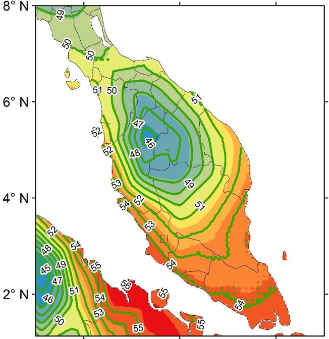
Atmosphere 2020, 11, 1012                                                                            2 of 21

feedback on global warming. Knowledge of the total vertical column of this parameter, also known as
integrated water vapour (IWV), and its variations, is particularly more useful than surface humidity in
the studies of radiation budget and the forecast of precipitation [6]. IWV variability and trends, which
are also significant in the exploration of climate change [7], form the central objective of this study.
      In recent years, many studies have been carried out to probe and detect changes in IWV by
deploying a variety of datasets retrievable from different sensors or platforms, including radiosonde [8,9],
microwave radiometers [10], Global Positioning Systems (GPS) [11–13], Raman Lidar [14], and satellite
remote sensing [15]. Traditionally, observation records from radiosondes represent an important
resource for monitoring the variability and trends in IWV because of its accuracy and vertical resolution.
It is not surprising, therefore, that observational records from this platform have been used by many
scholars as reference data in gauging the validity of IWV obtained from other techniques [16]. For instance,
the authors in [17] reported bias and root mean square errors of 0.68 and 4.47 kgm−2 , respectively,
for global tropical region when they evaluated ERA-Interim IWV against the radiosonde product.
      Many previous studies, using data from different platforms or sensors, have revealed both region
and time scale IWV trends. For instance, Rose and Elliott [18] used radiosonde observations to
establish an upward trend in IWV across most sites in the United States and Canada between 1973
and 1993. Similar positive trends, mostly in the Northern Hemisphere, have been reported [3,19].
Based on 27-year radiosonde observations in China, Xie et al. [20] also reported a significant upward
IWV trend from 1979 to 2005 in the northern part of China, with a reversed trend in the southern
part. Similarly, Chen and Liu [17] deployed precipitable water datasets from radiosonde, European
Centre for Medium-range Weather Forecast (ECMWF), National Centre for Environmental Prediction
(NCEP) reanalysis, GPS, and microwave satellite observations, for the period 1979–2014, to analyse
both variability and trend in global precipitable water and obtained positive global trends for all
five datasets. Generally, research efforts have pointed to upward water vapour trends, both at the
surface [1,3,18] and aloft [3].
      On average, precipitable water vapour content appears to produce positive trends globally,
consistent with global warming. However, such inferences may not be absolute, since various studies
deployed data from different sources and sites, with varying temporal and spatial coverages. More so,
most techniques or sensors deployed in gathering humidity data for the quantification and/or trend
analyses of IWV cited above suffer one form of limitation or the other. For instance, the data quality
of radiosonde networks is not only variable in the upper troposphere, but poor at extreme humidity
values [18]. Spatial limitations due to high operational cost and differences in instruments’ sensors over
time add to the heterogeneity of the network’s data quality. While observations from sun photometers
are limited to cloud-free regions, low spatial resolution restricts the use of space-based instruments.
Since the introduction of GPS as an efficient meteorological tool by [11], its data are frequently used
to determine precipitable water, among other atmospheric parameters. The temporal span of GPS
data, however, falls short of the minimum period (30 years) required to aggregate weather for the
evaluation of climatic effects in an area, as described by the World Meteorological Organization
(WMO) [21]. This period is deemed sufficiently long to filter interannual variations or anomalies and
thus, reveal climatic trends [22]. Due to frequent changes in data assimilation systems and models,
operational analyses from in situ and satellite observations are rather short in providing homogeneous
datasets on the atmospheric moisture budget. Retroactively produced (reanalysis) data, based on the
utilisation of the same model and data assimilation procedure, are, therefore, better in this respect [23].
Reanalysis datasets for atmospheric studies are produced by assimilating various types of observations
(ground and satellite) into a dynamically coherent dataset based on an atmospheric general circulation
model [24]. These datasets have been widely used in atmospheric studies like climate change because
they have the advantages of multivariable outputs, global coverage, and continuous records.
      The foregoing relevance of IWV in climate studies, amongst others, has endeared interests in its
measurement and evolution, both in space and time. Regrettably, however, the study of IWV variability
and trend in Peninsular Malaysia is rare despite being an area characterised by various climatic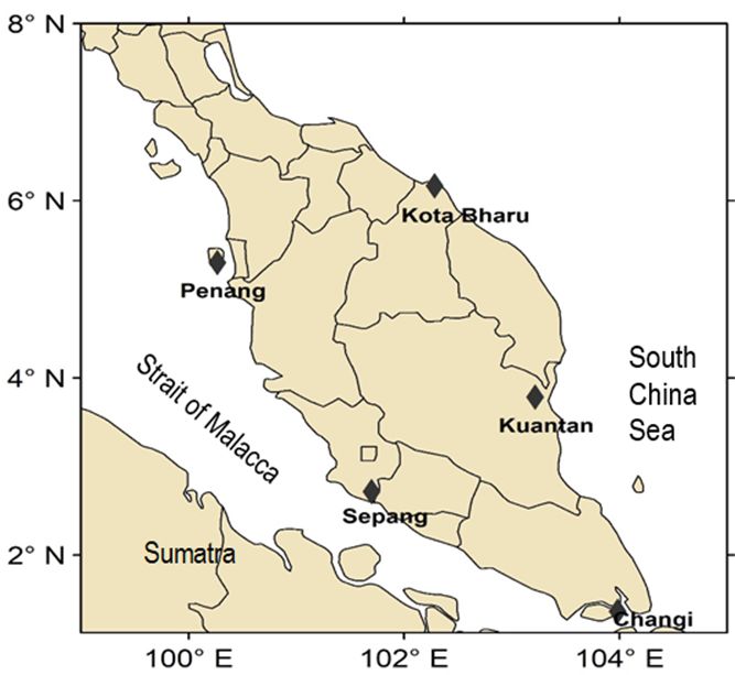
Atmosphere 2020, 11, 1012                                                                             3 of 21

features [25]. Aside from the very few reports on the quantification of IWV in the area, e.g., [26], there
are no existing studies on its variability and trend, let alone the deployment of ERA-Interim reanalysis
data. This is probably due to the limited number of in situ stations with traditionally long periods
of data records for meaningful exploration of variability and trends in IWV, unlike other regions in
the mid-latitude of the Northern Hemisphere. Peninsular Malaysia is an important area for climate
study, being a tropical region with overlapping seasonality and high topographic inhomogeneity.
Moreover, many global and regional phenomena, like El Niño, La Niña, and Indian Ocean Dipole, are
thought to influence the climate of the peninsular in addition to global warming. These proponents
could affect the severity of extreme events in the country [27]. Peninsular Malaysia, which stretches
from longitude 99–105◦ east of the meridian and from latitude 1–7◦ north of the equator, exhibits
two main seasons, the northeast monsoon (NEM) and southwest monsoon (SWM), flanked by two
inter-monsoon characteristics.
      The research area, which is situated in the equatorial doldrum region, is also characterised by
almost constant temperature year-round, having values between 24 and 32 ◦ C, with annual variation
of ~2 ◦ C. However, the east coast is often affected by cold surges originating from Siberia during the
NEM [28,29]. Vector winds and temperature patterns for the SWM and NEM seasons in the study area
are shown in Figure 1. The topography of Peninsular Malaysia is characterised by a series of mountains,
rising abruptly from the wider and flatter coastal plains. Prominent among these undulating surfaces
is the Titiwangsa Mountains, which run from the Malaysia–Thailand border in the north to the southern
state of Negeri Sembilan, effectively demarcating the area into western and eastern parts, as shown in the
inset of Figure 2. These mountains exert considerable influence on the local wind circulations in the region.
      In the current study, therefore, both radiosonde data from the Integrated Global Radiosonde
Archive (IGRA) version 2 and the ERA-Interim reanalysis product from ECMWF [30] for the period
1988–2018 are used to investigate variability and trends in IWV over Peninsular Malaysia. ERA is one
of the most advanced global atmospheric reanalysis records, which has been revised and improved
upon over the years and used elsewhere to evaluate both variability and trends in IWV [5,7,19,30].
Moreover, the data compare well with radiosonde observations [31]. This paper focuses on the
evaluation of the annual and seasonal means of IWV as well as its variations and long-term trends
over Peninsular Malaysia. Though analysis of seasonal variability helps to better identify regions
with higher uncertainty as well as understand the physical processes involved in different seasons
(e.g., the component responsible for moisture advection differs in wet and dry seasons) [31], it is
rarely provided in many other studies. In the current paper, interannual and seasonal (NEM and
SWM) variability in ERA and RS IWV are evaluated over Peninsular Malaysia. IWV observations from
the Advanced Television and Infrared Observation Satellite Operational Vertical Sounder (ATOVS)
are primarily used to evaluate the spatial representation of ERA IWV in the study region. Prior to
long-term trend analysis, the IWV from ERA is firstly compared with: (1) Retroactively produced IWV
retrieved from ATOVS instruments aboard the National Oceanic and Atmospheric Administration
(NOAA) and archived by the Satellite Application Facility on Climate Monitoring (CM-SAF), for the
period 2001–2011. (2) Radiosonde IWV (RS) observations from IGRA (1988–2018) for selected WMO
stations within and around Peninsular Malaysia. The paper is organised such that data description
and methodology are detailed in Section 2, while the results are presented and discussed in Section 3,
with conclusions drawn in Section 4.
Atmosphere 2020, 11, x FOR PEER REVIEW 4 of 23
Atmosphere 2020, 11, 1012 4 of 21
Atmosphere 2020, 11, x FOR PEER REVIEW 4 of 23
(a) (b)
(a) (b)
(c) (d)
(c) (d)
Figure 1. Distribution of mean wind speed (m/s) and direction (upper row) and mean temperature in
Figure
Figure
°C (lower Distribution
1. Distribution
1. row) for the ofofmean
meanwind
windspeed
southwest speed (m/s)
(m/s)
monsoon and
and
(SWM) direction
direction (upper
(upper
(a,c) and the row)row)
andand
northeast mean
mean temperature
temperature
monsoon in
(b,d) over
in ◦ C (lower row) for the southwest monsoon (SWM) (a,c) and the northeast monsoon (b,d) over
°C (lower row) for the southwest
Peninsular Malaysia from 1988 to 2018. monsoon (SWM) (a,c) and the northeast monsoon (b,d) over
Peninsular Malaysia
Peninsular Malaysia from
from19881988to
to2018.
2018.
Figure 2. Peninsular Malaysia showing integrated global radiosonde archives (IGRA) stations (filled
Figure 2. Peninsular Malaysia showing integrated global radiosonde archives (IGRA) stations (filled
Figure 2. Peninsular
diamond), from whichMalaysia showing
integrated integrated
precipitable global
water radiosonde
vapour (IWV) archives
data were(IGRA) stations
obtained. (filled
Inset is the
diamond), from which integrated precipitable water vapour (IWV) data were obtained. Inset is the
diamond), from which integrated
topographic map of the study area. precipitable water vapour (IWV) data were obtained. Inset is the
topographic
topographic map
map of
of the
the study
study area.
area.Atmosphere 2020, 11, 1012 5 of 21
2. Data and Methodology
The variability and trend studies of IWV are performed using 31 years of monthly means of
ERA and RS observations. The study area is shown in Figure 2, with the locations of IGRA stations
represented by dark-filled diamonds. Prior to the foregoing analyses, ERA IWV is compared with
RS and CM-SAF (SAF) IWV records. The coefficient of determination (R2 ), mean bias (MB), and root
mean square (RMS) errors have been used to gauge the level of agreement between the different pairs
of datasets. The sources, description, and methodologies used in acquiring the respective datasets are
described below.
2.1. Radiosonde
Daily radiosonde data for this study were obtained from the Integrated Global Radiosonde
Archive (IGRA) version 2 of the National Climatic Data Centre (NCDC, Asheville, NC, USA). The data
are available [32]. IGRA2 consists of almost 2700 global stations for both radiosonde and pilot
balloon observations, with a temporal span of over 60 years of records, which include temperature,
relative humidity, pressure, wind speed, and wind direction. The requisite IWV data were extracted
from twice-daily radiosonde observations at mandatory and significant levels from WMO stations
at Kota Bharu, Penang, Kuantan, Sepang, and Changi (Singapore) for the period 1st January 1988 to
31st December 2018. The datasets were retrieved along with metadata on background instrumentation
and station history, which helped in ensuring data quality through checks for inconsistencies such as
outliers and duplicate levels, among others.
Three stages of quality control were imposed on the daily data: Firstly, obvious errors, e.g.,
values of IWV 100 mm were discarded as invalid. Secondly, the monthly and annual mean
values of IWV for each station were calculated based on outputs from the first stage. Finally, outliers
were removed from the time series of eventual stations when the difference between their values
and the climatological mean was more than 3 standard deviations (σ) [33]. The systematic as well as
instrumental errors were, however, not considered in the quality control process. After the quality
control procedure, the data were further tested for homogeneity as follows: (1) Stations with obvious
inhomogeneous data were not considered. (2) Stations without complete twice daily records were
precluded. (3) At least 18 daily observations were used to calculate the mean monthly values. Any year
that had at least 10 valid months was used in deriving the mean values of IWV. (4) Data from stations
with a consistent time series of 11 years between 1988 and 2018 were considered for variational studies,
while a minimum of 19 years of data was used for trend analysis. After the homogeneity test, records
from four of the six WMO stations in Peninsular Malaysia were found useful in the computation of
IWV values for comparison with the ERA observations. Data from Changi airport in Singapore, which
lies at the fringe of the southern part of the study area, were equally subjected to quality examination
and found useful for inclusion in the inter-comparison and trend analysis.
The diurnal (1200 UTC) and nocturnal (0000 UTC) data were separately treated and found to
correlate excellently across the stations, with correlation coefficient r ≥ 0.93. Although, insignificant
differences in trend between 0000 and 1200 UTC have been reported [18]. Nonetheless, the daily value
was derived as the mean of the two observations for each day and then, converted into monthly means
to conform with those of ERA-Interim. Information on the data used, including station location, are
given in Table 1.Atmosphere 2020, 11, 1012 6 of 21
Table 1. Description of the datasets and their sources.
Data/Source Study Area/Location
Temporal/ Temporal
Longitude Latitude Instrument
Name Spatial Resolution Coverage
(Degree) (Degree)
Vaisala (RS80) 1988–1993
Kota Bharu 102.283 6.167
Vaisala (RS 92G) 1994–2018
Twice daily
Radiosonde/IGRA Vaisala (RS80) observations 1988–1993
Penang 100.267 5.300
Vaisala (RS 92G) (00 and 12 UTC) 1993–2018
Vaisala (RS80) 1988–1993
Kuantan 103.217 3.783
Vaisala (RS 92G) 1994–2018
Graw DMF09 2000–2019
Sepang 101.700 2.717
Vaisala (RS80) 1988–1994
Changi 103.983 1.367
Vaisala (RS 92G) 1994–2018
ERA-Interim Peninsular 6–hourly observations/
97–106◦ E 1–7◦ N NWP 1988–2018
Reanalysis/ECMWF Malaysia 79 × 79 km2
Peninsular Daily observations/
ATOVS/CM-SAF 97–106◦ E 1–7◦ N ATOVS 2001–2011
Malaysia 90 × 90 km2
2.2. CM-SAF from ATOVS
Homogenised satellite data records, SAF, were mainly used to validate ERA. This set of data
is retrieved and archived by CM-SAF from ATOVS instruments aboard NOAA and Meteorological
Operational (Metop) Satellites. The ATOVS suite of instruments, which comprises a High-Resolution
Infrared Radiation Sounder (HIRS), Advanced Microwave Sounding Unit A and B (AMSU-A/B),
and Microwave Humidity Sounder (MHS), represents infrared spectrometers and microwave radiometers.
These instruments contain enough information to infer IWV value. Retrievals over oceans rely on all
sensors, whereas retrievals over land surfaces are mainly based on cloud-free HIRS measurements.
On a global scale, radiosondes and ATOVS water vapour agree reasonably well, with systematic
differences of 0.5 kg m−2 and root mean square differences of approximately 4 kg m−2 [34]. The ATOVS
data records consist of precipitable water and temperature products defined at all longitudes and
for latitudes 80◦ N to 80◦ S. CM-SAF retrieves and provides global fields of daily mean IWV on a
cylindrical equal area projection of 90 × 90 km2 and 0.5 × 0.5 longitude–latitude grid. The dataset
is accompanied by an uncertainty estimate that reflects the retrieval uncertainty and the sampling
error, which is particularly important in tropical areas. They are constructed using a specific kriging
algorithm that is detailed in Li et al. [35] and expounded by Schröder et al. [15]. In this study, SAF data,
for the period 2001–2011, also known as a climate data record (CDR), were extracted for all available
latitudes over the entire study area shown in Table 1 and Figure 1. Though the CDR spans 13 years,
the first two years are plagued with so many temporal gaps and are, therefore, precluded in this
study. This set of data, freely ordered from the CM-SAF website [35] contain high-quality, validated,
homogeneous climate data based on carefully calibrated inter-sensor radiances. The daily data from
2001 to 2011 were re-gridded to 0.125◦ × 0.125◦ longitude–latitude and converted to mean monthly
array for compatibility with the ERA IWV data.
2.3. ERA-Interim Reanalysis
ECMWF initiated a project to bridge her previous reanalysis, ERA-40, which spanned 1957–2002,
with her next-generation extended reanalysis, ERA-Interim. The aim of the project was to improve
on vital aspects of the former. This success resulted from a combination of factors, which include the
use of 4D variational analysis to minimise errors, the use of variational bias correction for satellite
data (impact of observing system changes is reduced), and other improvements in data handling.
With the improvement, ERA can now incorporate regular and irregular meteorological data, offer
better humidity analysis, as well as effective representation of the hydrologic cycle and stratospheric
circulation. The product, a global atmospheric reanalysis of repute, is available from 1st January 1979
to 31st August 2019 and can be downloaded freely from the ECMWF Public Datasets web interface [36].Atmosphere 2020, 11, 1012 7 of 21
The IWV products from the ERA reanalysis are based on various water vapour measurements, which
include clear-sky radiance observations from geostationary and polar-orbiting sounders, and the images
of remote sensing satellites like the Special Sensor Microwave Imager (SSM/I), Total Ozone Mapping
Spectrophotometer (TOMS), TIROS Operational Vertical Sounder (TOVS), and High Resolution Infrared
Radiation Sounder. Detailed documentation is found in [30]. ERA has been used in several climate and
trend analysis studies [15,17]. A stream of monthly means IWV of daily means data at a 0.125◦ × 0.125◦
resolution in netCDF output for the extent of Peninsular Malaysia (see Table 1) was retrieved for the
period 1st January 1988 to 31st December 2018. A total of 372 mean monthly arrays, each consisting of
97 columns and 73 rows of IWV, were available for the evaluation of variability and trends.
2.4. Inter Comparison of Means and Variability of IWV
Precise knowledge of the accuracy of IWV derived from models prior to deploying reanalysis
data for trend evaluation is indispensable. As stated earlier, RS and SAF can measure, with acceptable
accuracy of the order of several millimetres, atmospheric water vapour contents. A validation of the
ERA IWV is, therefore, performed using RS and SAF observations to obtain a reliable interpretation
of the ERA data quality in the study area. Makama and Lim [25] obtained good agreement between
radiosonde IWV and CM-SAF IWV, with correlation coefficients ranging between 0.79 and 0.94 with
MB < 1 kgm−2 across different regions of Peninsular Malaysia when the two datasets were compared.
ERA is firstly interpolated onto the radiosonde sites to extract the IWV data and then, directly compared
with IWV measured at the stations. Five radiosonde stations were identified for this study (see Figure 1
and Table 1) for both the comparison and trend evaluations. Secondly, the SAF data were re-gridded to
match the ERA grids and direct comparison of the means applied. It is worthy of note that SAF and RS
IWV agree reasonably well in the current study area [25]. Unfortunately, only 11 years (2001–2011)
of this dataset were used for validation for the reason mentioned in Section 2.2. Standard statistical
metrics, MB and RMS errors, given in Equations (1) and (2), were used to validate ERA IWV against its
RS and SAF counterparts across the study area.
n
1X
MB = (IWV 0 − IWV ) (1)
n
i=1
v
n
t
1X
RMS = (IWV 0 − IWV )2 (2)
n
i=1
where IWV is integrated water vapour derived from ERA, IWV0 is integrated water vapour from either
RS or SAF observations, n is the number of data points, while IWV and IWV 0 represent the respective
mean values of the integrated water vapour from a pair of datasets.
2.5. Trend Analysis
Annual and seasonal trends were computed for each station from 1988 to 2018 in both the ERA and
RS time series. Monthly anomalies were computed as deviations from the corresponding long-term
monthly means over the 31-year period. Annual averages were then obtained from the monthly
anomalies, with at least 10 months of data required for each annual anomaly. Time series for seasonal
anomalies were similarly obtained for the NEM (November–April) and the SWM (May–October) by
averaging the monthly anomalies for that season, with at least four months required for each seasonal
anomaly. To detect the trend in the IWV time series, a non-parametric Mann–Kendall (M–K) test at
95% confidence level was imposed on both datasets. M–K, which is a rank-based process, applicable
even in skewed data, has been widely used in detecting monotonic trends in climate study [32,37].
An additional major benefit of this test in analysing temporal series is that cases of missing data and
seasonality are not considered.Atmosphere 2020, 11, 1012 8 of 21
Suppose integrated water vapour is observed over a time series x = xi , with i = 1, 2, 3, . . . , n as
data points and x j being the data point at time j, then the M–K test statistic (S) is given as
n−1 X
X n
S= sgn x j − xi (3)
i=1 j=i+1
where n is the sample size, while xi and x j are the respective values for years i and j, with j > i.
The values of the data are treated based on an ordered time series evaluation, where each value is
compared with all subsequent data values. The initial value of S is assumed to be 0 when there is no
trend and 1 or −1 when there is an upward or downward trend, respectively. Simply put, if the value
of a data point is higher or lower than the value that precedes it, then S is respectively incremented
or decremented by 1. S is, therefore, defined by the sign function, with values ranging between ±1,
depending on whether x j − xi is less, equal, or greater than zero, as given in Equation (4) [37].
>0
+ 1, x j − x i
sgn x j − xi = 0, x j − xi = 0 (4)
−1, x j − xi < 0
For a sample size upward of 30, the S statistic is normally distributed and the normalised test
statistic Z can be computed as follows:
σ , S>0
S−1
S
Z=
0, S = 0 (5)
S+1 , S < 0
σ S
The procedure for the M–K trend test assumes the existence of only one data value at a particular
time period. If, however, there is more than one data point (tie) in a given time period, the median
value is considered [38]. It is, however, important to calculate the probability associated with S and the
sample size n, to statistically determine the significance or otherwise of the trend. The value of the
variance of S (σ) was, therefore, obtained using Equation (6) [37] with n ≥ 10,
m
1 X
σ(S) = n(n − 1)(2n + 5) − tp tp − 1 2tp + 5 (6)
18
p=1
where m is number of tied groups (i.e., a set of sample data with same value), and tp is the number
of data points in the pth group. The probability associated with the variance was computed using
Equation (7) in XLSTAT (XLSTAT is a complete analysis and statistics add-in for Microsoft Excel).
This method is suitable for the IWV dataset in the current study, since the sample size is greater than
10 with very few ties.
2
eZ /2
f (Z) = √ (7)
2π
The Z score considers the detection of monotonic trends from the following hypothesis: null
hypothesis (H0 )—no monotonic trend (i.e., variables are independent and equally distributed) and the
alternative hypothesis (H1 )—monotonic trend exists (i.e., variables are dependent with inhomogeneous
distribution). The acceptance or otherwise of H0 is determined by computing the normalised probability
associated with the Z statistic from Equation (6). In this paper, the significance level (α) was set at 0.05
(i.e., 95% confidence level) such that Z > Zα/2 indicates no monotonic trend in the IWV data. H0 is,
therefore, rendered invalid when |Z0.025 | ≥ 1.96, meaning that the trend is significant.
In this study, the Theil–Sen (T–S) estimator, which is resistant to outliers, was used to determine
the magnitude of IWV trend. T–S, named after Henri Theil [39] and Pranab Sen [40], is a non-parametricAtmosphere 2020, 11, 1012 9 of 21
method usually deployed in finding a fit for heteroscedastic data. Suppose (t1 , y1 ), (t2 , y2 ), . . . , (tn , yn )
represent data points, then T–S estimates the slope of the line that connects each pair of data. The median
among the slopes of all the data pairs becomes the slope of the fit, given as
y j − yi
β̂ = med (8)
1≤i< j≤n t j − ti
Knowing the value of the slope, the intercept was calculated as b̂ = yi − β̂ti , where t is time of
observation. The sign of β̂ reveals whether the change is positive or negative and its magnitude shows
how steep the change is [41].
3. Results and Discussion
3.1. Comparison of IWV from ERA with RS and SAF Observations
The comparison between monthly means IWV from ERA with those from RS and SAF was done
using the statistical evaluation metrics provided in Equations (1) and (2). The objective here is to
check the reliability and consistency of the ERA observations against RS and SAF measurements,
as mentioned earlier. Again, note that SAF, being available from 2001 to 2011, was only used in the
validation of ERA and not in long-term trends, due to its temporal limitation.
3.1.1. Evaluation of IWV Means
The comparison between the means of IWV from ERA, RS, and SAF for the five stations is
summarised in Table 2, with the visual fits depicted in Figure 3. Table 2 presents values of the statistical
indices for each of the five stations, including the number of observations, when the monthly means
of IWV from RS and SAF were compared with those from ERA for the entire study period. Figure 3,
on the other hand, shows the corresponding scatterplots for the monthly means of IWV from RS and
SAF against those from ERA. On the bases of MB (Table 2), ERA is wet against RS and dry against
SAF, with respective greatest values of −2.85 kg m−2 found at Changi and 1.94 kg m−2 at Sepang.
While the average MB for all the stations in the RS/ERA comparison is well below 1 kg m−2 , that of
Changi is up by a scale of ~3. In the SAF/ERA comparison, the average MB is ~1.22 kg m−2 across
all stations, with the smallest and largest values being 0.63 and 1.94 kg m−2 in Kuantan and Sepang,
respectively. From the goodness of fits in Table 2, a proximity between the IWV from ERA and those
from RS and SAF across all stations are revealed, except for a relative departure at Changi, where
highest RMS for RS/ERA and SAF/ERA are 4.05 and 2.43 kg m−2 , respectively. Moreover, the slopes
in Figure 3 are close to 1, indicating that the data points are distributed around the 1:1 line, and the
maximum deviations of ERA are less than two standard deviations from the means of both the RS and
SAF. The slopes of the linear regression lines for the RS/ERA comparison shown in Figure 3 (left panel)
are all below 1, ERA on average being wetter than RS with relatively larger differences at lower IWV
values. A likely reason is the impairment of time-lag response suffered by radiosonde sensors as
they ascend the atmosphere, during which IWV is underestimated [42]. However, the slopes of the
linear fits for the SAF/ERA pairing, shown on the right panel in Figure 3, are above 1 for Kota Bharu,
Penang, and Sepang, ERA being persistently drier particularly at higher IWV. This is probably due to
the interpolation scheme used in filling void data points caused by heavy precipitation in the ATOVS
measurements. The SAF IWV, retrieved from ATOVS, has in addition to sampling gaps, data void
points due to strong scattering events like heavy precipitation [43]. A kriging interpolation scheme is
used to fill these void points. The scheme uses valid observations in the vicinity of the gaps, whose
neighbouring areas are typically humid, and fills them up with generally larger values of IWV than
the valid observation during an overpass, thereby causing a systematic bias at higher IWV values.
Although the seemingly larger bias at lower IWV for Kuantan and Changi, based on their slopes (>1),
is difficult to explain, the grid altitude of ERA and the surface pixel of ATOVS, which are not factored
into the current comparison, are likely suspects. The highest and lowest values of R2 in the RS/ERAAtmosphere 2020, 11, x FOR PEER REVIEW 10 of 23
Atmosphere 2020, 11, 1012 10 of 21
into the current comparison, are likely suspects. The highest and lowest values of R2 in the RS/ERA
comparisonare
comparison arefound
foundatatPenang
Penang(0.902)
(0.902) and
and Changi
Changi (0.845),
(0.845), respectively,
respectively,while
whilethe
thecorresponding
corresponding
values for the SAF/ERA are seen in Kota Bharu (0.898) and Changi (0.789).
values for the SAF/ERA are seen in Kota Bharu (0.898) and Changi (0.789).
Table 2. Statistical proximity between IWV (Integrated water vapour) from ERA (1988–2018) when
Table 2. Statistical proximity between IWV (Integrated water vapour) from ERA (1988–2018) when
compared to RS (1988–2018) and SAF (2001–2011) IWV observations in Peninsular Malaysia. n is
compared to RS (1988–2018) and SAF (2001–2011) IWV observations in Peninsular Malaysia. n is
number of observations.
number of observations.
RS/ERA SAF/ERA
RS/ERA SAF/ERA
Station MB RMS MB RMS
Station n MB−2) RMS
n MB RMS
n (kgm (kgm−2)
n (kgm )
−2 (kgm−2)
(kgm−2 ) (kgm−2 ) (kgm−2 ) (kgm−2 )
Kota Bharu 360 −0.40 2.04 132 0.87 1.91
Kota Bharu 360 −0.40 2.04 132 0.87 1.91
Penang
Penang
372
372
−−0.30
0.30 1.50
1.50
132
132 1.33
1.33
1.87
1.87
Kuantan
Kuantan 336
336 −−0.77
0.77 1.72
1.72 132
132 0.630.63 1.42 1.42
Sepang
Sepang 228
228 −1.06
−1.06 2.09
2.09 132
132 1.941.94 2.01 2.01
Changi 372 −2.85 4.05 132 1.34 2.43
Changi 372 −2.85 4.05 132 1.34 2.43
60 (a) Changi 60 (f) Changi
48 48
y = 0.889x + 4.664 y = 0.896x + 1.643
36 R2 = 0.845 36 R2 = 0.789
60 (b) Sepang 60 (g) Sepang
48 48
y = 0.984x − 1.052 y = 1.089x − 5.450
36 R2 = 0.848 36 R2 = 0.808
ERA IWV (kg m−2)
60 (c) Kuantan 60 (h) Kuantan
48 48
y = 0.956x + 1.600 y = 0.892x + 2.835
36 R2 = 0.873 36 R2 = 0.887
60 (d) Penang 60 (i) Penang
48 48
y = 0.897x + 3.913 y = 1.091x − 4.984
36 R2 = 0.902 36 R2 = 0.883
60 (e) Kota Bharu 60 (j) Kota Bharu
48 48
y = 0.915x + 3.459 y = 1.038x − 2.333
36 R2 = 0.853 36 R2 = 0.898
30 40 50 60 30 40 50 60
Radiosonde (RS) IWV (kg m ) −2
CM-SAF (SAF) IWV (kg m−2)
Figure
Figure 3. 3.Scatterplots
Scatterplotsofofmonthly
monthly means
means ofof IWV
IWV from
from ERA comparedwith
ERA compared withIWV
IWVfrom:
from:Radiosonde
Radiosonde
((left) panel) and CM-SAF ((right) panel) for the five selected WMO stations in Peninsular Malaysia.
((left) panel) and CM-SAF ((right) panel) for the five selected WMO stations in Peninsular Malaysia.
Although
Although ERAERAagrees wellwell
agrees with with
RS andRSSAFandproducts across the
SAF products stations,
across the on average,onit overestimates
stations, average, it
IWV by 1.29 kg IWV −2
m relative to m
RS and its estimate −2 against −2
overestimates by 1.29 kg −2 relative to RS andisits
understated by 1.22 kg m
estimate is understated by 1.22 kg m SAF in the
against
entire
SAF study
in the area.
entire Whereas
study area.higher RMShigher
Whereas values are values
RMS obtained are from RS/ERA
obtained fromevaluation, the SAF/ERA
RS/ERA evaluation, the
comparison presents relatively
SAF/ERA comparison presentshigher amplitudes
relatively of mean IWV.
higher amplitudes At theIWV.
of mean spatial
At front, the performance
the spatial front, the
of performance
ERA againstofRS ERA
andagainst
SAF isRSnoted
and SAF is noted to
to degrade degrade
slightly slightly southwards
southwards with relatively
with relatively better at
better results
theresults at thestations
northern northern stations
(Kota (Kota
Bharu andBharu
Penang)and Penang)
compared compared
to Sepangto Sepang and Changi,
and Changi, whichwhich are
are located
at located at lowerinlatitude
lower latitude in the peninsular.
the peninsular. These are
These stations stations
at theare at the southern
southern fringe offringe of Peninsular
Peninsular Malaysia,
Malaysia,
where where precipitation
precipitation is usually
is usually high, mainlyhigh, mainly
due to due tostorms.
convective convective
The storms. The pronounced
pronounced values of wet
MB in the ERA/RS comparison are likely due to the inability of radiosonde to capture the relatively
high moisture content [17,44] at the two stations. On the other hand, the large dry biases in the sameAtmosphere 2020, 11, 1012 11 of 21
stations for the ERA/SAF pairing may be due to kriging interpolation in addressing void data points
in the ATOVS IWV retrievals as stated earlier. Moreover, HIRS signals are known to saturate at very
high IWV [15,34], where the additional information from other observations in ERA becomes the only
source of reliable values of IWV. Based on the evaluation metrics, the performance of ERA against
SAF is more spatially consistent across the stations than between ERA and RS. Representativeness
uncertainty arising from the pairing of RS (point observation) with ERA (areal observation) across the
radiosonde stations is most likely to cause the observed spatial inconsistency in the RMS values. To the
authors’ knowledge, the representativeness uncertainty is unknown at each IGRA station. However,
the authors in [45] reported strong dependency of representativity uncertainty, for specific humidity,
on height and weather condition, which have not been considered in this study. Other sources of
biases found across the stations in the SAF/ERA IWV comparison include differences in sampling daily
data as well as the different temporal periods between ERA and SAF. While daily mean ERA IWV are
derived from four equally distributed fields (00, 06, 12, and 18 UTC), unequally distributed orbits are
used to construct daily means of SAF IWV [15]. Additionally, the restriction of the ATOVS-derived
IWV over land to only cloud-free HIRS observations is also an important source of measurement
uncertainty, as weather conditions were not considered in the current comparison. The MB and RMS
errors are generally within those reported by [17], who compared ERA with RS for global tropical
regions and for the global agreement between ERA and SAF [15].
Most of the discrepancies noted in the RS/ERA comparison are likely from instrumental uncertainties
associated with RS measurements, among others. For instance, the absence of radiation/rain shielding for
the capacitive sensor in the RS92 may also contribute to its poor performance at moisture extremes,
as documented in Miloshevich et al. [46] and Liu and Tang [47]. They also reported errors in the
measurement of humidity at the upper troposphere due to solar heating of the Vaisala RS92 sensor,
which is not equipped with the radiation/rain shielding found on the earlier sensor (RS80). Although
the authors in [46] have proposed empirical procedures to correct such errors, these are, however, not
applied in the current study. Horizontal drift of the radiosonde balloon from the launch point is also
an additional source of errors [48] in the RS/ERA evaluation
Finally, the errors in both ERA and SAF are suspected in areas where data are sparse, and/or
regions with poor performance in model physics and dynamics, which are difficult to diagnose e.g., [31].
The observed differences between ERA and SAF may, therefore, be linked to differences in model
physics and data assimilation. The presence of seasonal differences in the quality of relative humidity
measurements by radiosondes [49,50] calls for both seasonal and annual performance evaluations of
ERA IWV.
3.1.2. Evaluation of Seasonal and Interannual Means
Although four seasons (NEM, pre-monsoon, SWM, and early NEM) have been identified for
Peninsular Malaysia [51], the present comparison is based on the NEM (November–April) and the
SWM (May–October). The seasonal and interannual variations of IWV from RS and SAF using
the matched sample with the ERA reanalysis product, for the entire study period, are presented in
Figure 4. Conspicuous seasonal variations are revealed by all three datasets (Figure 4a) in an apparently
synchronised oscillation but with different amplitudes. A steady rise in IWV begins in March and
peaks in May, marking the beginning of the SWM when a large quantity of moisture is squeezed into
Peninsular Malaysia. IWV, thereafter, slides gradually and dips in August, before another climb that
peaks in November at the retreat of the SWM and the beginning of the NEM in the region. All three
datasets accurately capture the seasonal variations in IWV as well as the moisture changes in the
two seasons. While ERA maintained a consistent wet bias against RS in both seasons, SAF on the
other hand is wetter than ERA during the SWM and drier for most part of the NEM. Furthermore,
the MB values from both the RS and SAF evaluation of ERA are obviously larger in the SWM season,
during which quantity of moisture is noted to be higher in Peninsular Malaysia. This is consistent
with the interannual comparison, depicted in Figure 4b, which shows a common oscillation of IWVAtmosphere 2020, 11, x FOR PEER REVIEW 12 of 23
Atmosphere 2020, 11, 1012 12 of 21
interannual comparison, depicted in Figure 4b, which shows a common oscillation of IWV from both
datasets. Abrupt drops in IWV value observed from 2003 to 2004 and in 2015 may be due to El Niño
from both datasets. Abrupt drops in IWV value observed from 2003 to 2004 and in 2015 may be due
(El Niño is a large-scale ocean–atmosphere climate interaction associated with episodic warming in
to El Niño (El Niño is a large-scale ocean–atmosphere climate interaction associated with episodic
sea surface temperatures across the central and east–central Equatorial Pacific, which often results in
warming in sea surface temperatures across the central and east–central Equatorial Pacific, which often
warm and dry conditions.) events. Records from the Oceanic Niño Index (ONI) indicate the
results in warm and dry conditions.) events. Records from the Oceanic Niño Index (ONI) indicate
occurrence of very strong Niño events across the study area within the period of observation,
the occurrence of very strong Niño events across the study area within the period of observation,
particularly in 2004 and 2015 [52]. Moreover, the Malaysian Meteorology Department (MMD, 2009)
particularly in 2004 and 2015 [52]. Moreover, the Malaysian Meteorology Department (MMD, 2009) [53]
[53] also reported El Niño events in 2003–2004. These events are known to have caused severe drought
also reported El Niño events in 2003–2004. These events are known to have caused severe drought
across Indonesia, Philippines, Malaysia, and other adjoining regions [52]. Overall, the ERA IWV
across Indonesia, Philippines, Malaysia, and other adjoining regions [52]. Overall, the ERA IWV
exhibits phasal interannual variation but with consistent respective dry and wet biases relative to the
exhibits phasal interannual variation but with consistent respective dry and wet biases relative to
SAF and RS products, which is in line with the results presented in Section 3.1.1. Generally, the results
the SAF and RS products, which is in line with the results presented in Section 3.1.1. Generally,
show better seasonal compatibility in NEM against the SWM season, as evident in the seasonal
the results show better seasonal compatibility in NEM against the SWM season, as evident in the
matches shown in Figure 4a. Aside from the potential dependency of the uncertainty of radiosonde
seasonal matches shown in Figure 4a. Aside from the potential dependency of the uncertainty of
observations on IWV, it can be argued that seasonal differences in MB and RMS errors are dominated
radiosonde observations on IWV, it can be argued that seasonal differences in MB and RMS errors are
by the increasing IWV values in the SWM season. During this period, the natural variability of water
dominated by the increasing IWV values in the SWM season. During this period, the natural variability
vapour also increases and this increase in natural variability enhances the representativity uncertainty
of water vapour also increases and this increase in natural variability enhances the representativity
between RS and ERA, which are, respectively, point and areal observations. Furthermore, the large
uncertainty between RS and ERA, which are, respectively, point and areal observations. Furthermore,
dry bias in ERA relative to SAF during most of the period of the SWM may either be due to the use of
the large dry bias in ERA relative to SAF during most of the period of the SWM may either be due to
kriging interpolation to fill up void data points or because the HIRS signal became saturated at very
the use of kriging interpolation to fill up void data points or because the HIRS signal became saturated
high water vapour values [15] or both. Different spatial resolutions between ERA and SAF (see Table
at very high water vapour values [15] or both. Different spatial resolutions between ERA and SAF
1) can also cause the observed discrepancies.
(see Table 1) can also cause the observed discrepancies.
60
(a)
Mean monthly IWV (kg m )
-2
54
48
ERA RS SAF
42
Jan Feb Mar Apr May Jun Jul Aug Sep Oct Nov Dec --
60
(b)
Mean annual IWV (kg m )
-2
54
48
ERA RS SAF
1988 1992 1996 2000 2004 2008 2012 2016 2020
Figure 4. (a) Seasonal cycle of monthly mean and (b) Annual mean time series of IWV over Peninsular
Figure 4. (a) Seasonal cycle of monthly mean and (b) Annual mean time series of IWV over Peninsular
Malaysia for ERA-Interim (1988–2018), radiosonde (1988–2018), and CM-SAF (2001–2011) observations.
Malaysia for ERA-Interim (1988–2018), radiosonde (1988–2018), and CM-SAF (2001–2011)
observations.
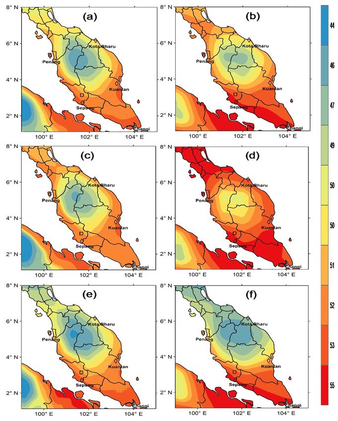
Figure 5 presents the mean of annual (a,b) and seasonal (c–f) IWV distributions from ERA and SAF.
In the maps of the means, it is seen that ERA reproduces the spatial variability well compared to SAF,
Figurethe
including 5 presents the mean
rich gradients of annual
in IWV, (a,b) and
particularly seasonal
in the north(c–f) IWV
central distributions
region, fromorography
where steep ERA and
SAF. In the maps of the means, it is seen that ERA reproduces the spatial variability well compared toAtmosphere 2020, 11, x FOR PEER REVIEW 13 of 23
Atmosphere 2020, 11, 1012 13 of 21
SAF, including the rich gradients in IWV, particularly in the north central region, where steep
orography manifests (e.g., Gunong Tahan, located in the north central area, along the Titiwangsa
manifests (e.g., Gunong Tahan, located in the north central area, along the Titiwangsa mountains).
mountains). This pattern is replicated during the SWM (Figure 5c,d) and NEM (Figure 5e,f), though
This pattern is replicated during the SWM (Figure 5c,d) and NEM (Figure 5e,f), though with different
with different intensities. From Figure 5, it is observed that ERA is generally drier than SAF at the
intensities. From Figure 5, it is observed that ERA is generally drier than SAF at the annual and SWM
annual and SWM periods, but wetter during the NEM season. Again, these observations are in
periods, but wetter during the NEM season. Again, these observations are in conformity with the
conformity with the seasonal time scale variational differences reported above.
seasonal time scale variational differences reported above.
Figure 5. Comparison of the spatial evolution of integrated water vapour (IWV) between (a,c,e):
Figure 5. Comparison of the spatial evolution of integrated water vapour (IWV) between (a,c,e): ERA-
ERA-Interim (1988–2018) and (b,d,f): CM-SAF (2001–2011). The first row is for mean annual values,
Interim (1988–2018) and (b,d,f): CM-SAF (2001–2011). The first row is for mean annual values, while
while the second and third rows are for SWM and NEM, respectively.
the second and third rows are for SWM and NEM, respectively.
The differences observed during seasonal comparison could arise from many factors, some of
The differences observed during seasonal comparison could arise from many factors, some of
which are easily discernible, while a lot more are hard to explain. Aside from the possible instrumental
which are easily discernible, while a lot more are hard to explain. Aside from the possible instrumental
errors from radiosonde sensors identified in Section 3.1.1, the SAF (satellite derived) IWV is not absolved
errors from radiosonde sensors identified in Section 3.1.1, the SAF (satellite derived) IWV is not
from some of these discrepancies. For instance, changes in the infrared (IR) surface emissivity can strongly
absolved from some of these discrepancies. For instance, changes in the infrared (IR) surface
influence the retrieval of the mean precipitable water at the lower troposphere. Bennartz et al. in [34]
emissivity can strongly influence the retrieval of the mean precipitable water at the lower troposphere.
have reported that retrievals of IWV using IR window channels have respective sensitivity of 0.6 and
Bennartz et al. in [34] have reported that retrievals of IWV using IR window channels have respective
2 kg m−2 emissivity changes in the two HIRS window channels. Using the IR emissivity databases,
sensitivity of 0.6 and 2 kg m−2 emissivity changes in the two HIRS window channels. Using the IR
they were able to show that the variability of surface emissivity in the window channels is ~1%,
emissivity databases, they were able to show that the variability of surface emissivity in the window
which could lead to uncertainties due to the sensitivity in the channels. The retrieval by Li et al. [35],
channels is ~1%, which could lead to uncertainties due to the sensitivity in the channels. The retrievalAtmosphere 2020, 11, 1012 14 of 21
as employed in the SAF data, uses a constant surface emissivity of 0.99 for the window channels. Such
small deviations from this value can cause large changes in IWV estimates, particularly in the lower
layer of the atmosphere. Additionally, the IR channels’ emissivity varies with changing vegetation
cover and cloudy sky, which are not considered in the satellite retrieval scheme [54]. Different periods
used for the comparison between ERA (1988–2018) and SAF (2001–2011) could also influence the bias.
Arising from the evaluated differences between the three datasets, ERA-Interim data are found to be
suitable for IWV analysis in the study area within the selected period and are, therefore, deployed in
the evaluations of its variability and trend. RS IWV for the same period is also used along with ERA
for the long-term trend evaluation.
3.2. Variability of IWV for the 31-Year Period
3.2.1. Temporal Variation
From Figure 4a in Section 3.1.2, which presents mean monthly cycle, it is obvious that IWV exhibits
double oscillations, with pairs of minima and maxima for both datasets. ERA presents a primary
minimum of 46.47 kgm−2 found in February. According to [29] and [55], this period is characterised by
the lowest amount of rainfall in the peninsular, with a peak in November of each year. The amount
of IWV engages a persistent increase from its lowest value in February until April and peaks in May,
marking the secondary maximum throughout the region. The parameter dips slightly to its secondary
minimum in August, coinciding with the second period of low precipitation as reported by [29].
The primary maximum is found in November, with the annual mean being 51.69 kgm−2 . This value is
consistent with the 51.28 kg m−2 reported by [56], who deployed GPS measurements between 2011
and 2014 to evaluate IWV in Peninsular Malaysia. Except for the different annual mean values of IWV
presented by each of the datasets, their oscillations are fairly synchronous throughout (Figure 4b).
Makama and Lim [25] reported similar cycles for RS and SAF when they compared IWV profiles from
the two datasets for the same study location.
The primary maximum found in November, which also coincided with the second peak of
precipitation, may be due to the retreat of the SWM and the equator-ward migration of the NEM wind,
as can be seen in Figure 1b. The transition of these monsoons enhances the formation of a wide area of
convergence that favours convection. Furthermore, the interactions between local topography and the
prevailing north-easterly wind across the South China sea, from the abundant moisture squeezed into
the region, may account for the high IWV at the onset of the NEM period. The primary minimum,
observed in February, may indicate the retreat of the above prevailing circulations. Factors such as
coastal upwelling and circulation aloft, which becomes divergent, and subsidence because of frequent
occurrence of inversions and isothermals in the upper atmosphere [57], may be responsible for the dip
in moisture at the retreat of the two monsoon seasons. It is worth noting that May and November are
the respective beginnings of the SWM and the NEM seasons [58].
3.2.2. Spatial Variation
Figure 6 illustrates the spatial distribution maps of seasonal mean IWV from ERA IWV data for the
NEM and SWM seasons during the 1988–2018 period. IWV decreases generally in a southeast–northwest
orientation over Peninsular Malaysia, with the regional maximum appearing over the southeastern
tip of the area in both seasonal distributions of the means. Complex and steep orography tends to
shape the intense horizontal gradient along the edges of the peninsular. The rich horizontal gradients
that manifest along the western boundary are relatively more intense in the SWM (Figure 6b) than
the NEM (Figure 6a) and the annual (contours not shown) time scales. Weak horizontal gradients are
easily noticed over the southern and central parts of the area in both seasons. Regional minima of IWV
are, however, seen as they manifest local elevations, which is evidently noticed around the central
regions (see Figure 1 inset). More water vapour is accounted for during the SWM than in the NEM,
which is consistent with the seasonal cycle shown in Figure 4a.Atmosphere 2020, 11, 1012 15 of 21
Atmosphere 2020, 11, x FOR PEER REVIEW 15 of 23
46
(a) NEM (b) SWM
49
51
53
55
Figure 6. Seasonal-mean ERA-Interim IWV for (a) NEM (November–April) and (b) SWM (May–October)
Figure 6. Seasonal-mean
for the 31-year (1988–2018)ERA-Interim IWV for (a)
period over Peninsular NEM (November–April)
Malaysia. and
Contours, in kg m−2 (b)
, are SWM
also (May–
shown.
October) for the 31-year (1988–2018) period over Peninsular Malaysia. Contours, in kg m−2, are also
shown.
The northward transport of water vapour, as can be seen in Figure 1a, may be responsible for the
abundant water vapour with associated large horizontal gradients over the southeastern part of the
The northward
peninsular during thetransport of water
SWM season. Thisvapour, as can be
water vapour seen in is
transport Figure
linked1a, may
with thebelow-level
responsible for the
monsoon
abundant
flow and the water
steepvapour with associated
topographic large horizontal
slopes of Titiwangsa mountains,gradients
whichover the southeastern
run from part of the
the Malaysia–Thailand
peninsular during the SWM season. This water vapour transport is linked
border to the southern state of Negeri Sembilan (Figure 2 inset), blocking its farther northwestward with the low-level monsoon
flow and the
intrusion. steep topographic
Generally, elevations are slopes of Titiwangsa
relatively lower to mountains,
the south than which run from
towards the Malaysia–
the northern part,
Thailand border to the southern state of Negeri Sembilan (Figure 2 inset),
forming a southwest–northeast orientation of horizontal precipitable water gradients. It is, therefore, blocking its farther
northwestward
not surprising that intrusion.
areas withGenerally, elevations are
lower topography relatively
present higherlower
IWV,tosince
the south than towards
more moisture content the
northern part, forming
tends to reside in the lower a southwest–northeast
troposphere. orientation of horizontal precipitable water gradients.
It is, Within
therefore, not surprising that areas with
the peninsular, on the other hand, a relatively lower topography
dry moisture present
regime higher
tendsIWV, since more
to manifest high
moisture content tends to reside in the lower troposphere.
topography, as mentioned earlier. The seemingly dry IWV during the NEM season over areas like
Within
Kelantan andthe peninsular,which
Terengganu, on theareother
on thehand, a relatively
eastern coast ofdrythe moisture
peninsular, regime
despitetends
theirtohigher
manifest high
rainfall
topography, as mentioned earlier. The seemingly dry IWV during the NEM
amounts at this period [55], may be ascribed to higher topography that typifies the region. Moreover, season over areas like
Kelantan
during this and Terengganu,
season, the meanwhich wind are flow,oncontrolled
the eastern coastentirely
almost of the by peninsular, despite their
the northwesterlies thathigher
later
rainfall amounts at this period [55], may be ascribed to higher topography
transits into northeasterlies on reaching Peninsular Malaysia, as seen in Figure 1b, may be responsible that typifies the region.
Moreover, duringdry
for the apparent thisIWV
season, theregion.
in the mean wind On the flow, controlled
other almost entirely
hand, relatively high IWV by the northwesterlies
is observed in the
that later parts
northern transitsof into northeasterlies
the peninsular during on reaching
the SWMPeninsular Malaysia,
period, despite sloweras wind
seen in Figure
speed 1b, may to
compared be
responsible for the apparent dry IWV in the region. On the other hand,
the NEM wind [59,60]. This is because the SWM winds, which arrive at Peninsular Malaysia from relatively high IWV is observed
in
thethe northern parts
Indonesian Islandofofthe peninsular
Sumatra (see during
Figure the1a),SWM period,
experience despite slower
a moisture windeffect
sheltering speedcreated
compared by
to the NEM wind [59,60]. This is because the SWM winds, which arrive
high mountain ranges [29]. Moreover, as the Strait of Malacca widens northwards, the land–sea at Peninsular Malaysia from
the Indonesian
breeze Island of
and convection Sumatra
exert (see Figure
local influence, to 1a), experience
a large extent, on a moisture
atmospheric sheltering
moisture effect
[61].created
More so, by
high mountain ranges
the prevalently higher[29]. Moreover,in
temperatures asthe
thenorthern
Strait of Malacca widens northwards,
area, particularly during thisthe land–sea
period, breeze
as seen in
and convection exert local influence, to a large extent, on atmospheric
Figure 1c, could induce evaporation rate and consequently, produce more moisture content aloft. moisture [61]. More so, the
prevalently higher temperatures in the northern area, particularly during this period, as seen in Figure
3.3.could
1c, Long Term
induceTrends in ERA and
evaporation rateRS and IWV (1988–2018)produce more moisture content aloft.
consequently,
Durre et al. [8] observed that for a better understanding of climate dynamics, it is important
3.3. Long Term Trends in ERA and RS IWV (1988–2018)
to investigate long-term trends in precipitable water vapour. Linear trends between 1988 and 2018
Durre et
in monthly al. [8] observed
anomalies from ERAthatand
for RS
a better
IWVsunderstanding
are, therefore,of climate dynamics,
performed it is important
for each station using the to
investigate long-term
non-parametric M–K andtrends
T–Sin precipitable
tests. watersignificance
The statistical vapour. Linear
of thetrends
trendsbetween
and the 1988 and 2018
T–S slope in
(β) for
monthly anomalies
both annual from ERA
and seasonal time and RSare
scales IWVs are, therefore,
presented in Table performed
3, while thefor eachtime
annual station using
series thewith
along non-
parametric M–K and
the corresponding T–S tests.
p-values areThe statistical
depicted significance
in Figure of the
7. Trends trends
were alsoand the T–S
obtained in slope
both the(β) for both
annual
annual and seasonal time scales are presented in Table 3, while the annual time series along with the
corresponding p-values are depicted in Figure 7. Trends were also obtained in both the annual andYou can also read