Theia Snow collection: high-resolution operational snow cover maps from Sentinel-2 and Landsat-8 data
←
→
Page content transcription
If your browser does not render page correctly, please read the page content below
Earth Syst. Sci. Data, 11, 493–514, 2019
https://doi.org/10.5194/essd-11-493-2019
© Author(s) 2019. This work is distributed under
the Creative Commons Attribution 4.0 License.

        Theia Snow collection: high-resolution operational snow
            cover maps from Sentinel-2 and Landsat-8 data
           Simon Gascoin1 , Manuel Grizonnet2 , Marine Bouchet1 , Germain Salgues2,3 , and Olivier Hagolle1,2
                      1 CESBIO,   Université de Toulouse, CNRS/CNES/IRD/INRA/UPS, Toulouse, France
                                                    2 CNES, Toulouse, France
                                                 3 Magellium, Toulouse, France

                              Correspondence: Simon Gascoin (simon.gascoin@cesbio.cnes.fr)

                                Received: 22 November 2018 – Discussion started: 29 November 2018
                            Revised: 16 March 2019 – Accepted: 20 March 2019 – Published: 16 April 2019

       Abstract. The Theia Snow collection routinely provides high-resolution maps of the snow-covered area from
       Sentinel-2 and Landsat-8 observations. The collection covers selected areas worldwide, including the main
       mountain regions in western Europe (e.g. Alps, Pyrenees) and the High Atlas in Morocco. Each product of
       the Theia Snow collection contains four classes: snow, no snow, cloud and no data. We present the algo-
       rithm to generate the snow products and provide an evaluation of the accuracy of Sentinel-2 snow products
       using in situ snow depth measurements, higher-resolution snow maps and visual control. The results suggest
       that the snow is accurately detected in the Theia snow collection and that the snow detection is more accu-
       rate than the Sen2Cor outputs (ESA level 2 product). An issue that should be addressed in a future release
       is the occurrence of false snow detection in some large clouds. The snow maps are currently produced and
       freely distributed on average 5 d after the image acquisition as raster and vector files via the Theia portal
       (https://doi.org/10.24400/329360/F7Q52MNK).

1   Introduction                                                    last access: 12 April 2019) shed light on the user require-
                                                                    ments for snow services based on satellite remote sensing.
The snow cover is an important driver of many ecological,           SCA and fSCA products were ranked as the most impor-
climatic and hydrological processes in mountain regions and         tant by the respondents (Malnes et al., 2015). The survey
in high latitude areas. In these regions, in situ observations      also indicated the need for operational products provided on
are generally insufficient to characterize the high spatial vari-   a daily basis, with latency times shorter than 12 h. High-
ability of the snowpack properties. The snow cover was in-          resolution data down to 50 m resolution were sought by road
cluded as one of the 50 essential climate variables (ECVs)          and avalanches authorities (Malnes et al., 2015). The respon-
to be monitored by satellite remote sensing by the Global           dents requested regional products, e.g. on the scale of entire
Observing System for Climate (GCOS) in accordance with              mountain ranges like the Alps or even the whole of Europe,
the Committee on Earth Observation Satellites (CEOS) agen-          and preferred the Universal Transverse Mercator (UTM) pro-
cies. ECVs are intended to support the work of the United           jection (Malnes et al., 2015). At the national level in France
Nations Framework Convention on Climate Change and the              there is also a need for operational high-resolution snow-
Intergovernmental Panel on Climate Change.                          covered area maps as revealed by the recent roadmap for
   The snow cover is not a variable sensu stricto, but an ob-       satellite applications issued by the French Government (Plan
ject which can be characterized through many variables, in-         d’applications satellitaires 2018, Commissariat général au
cluding snow-covered area (SCA), fractional area (fSCA),            développement durable, 2018). Based on a wide panel of end
albedo, liquid water content, snow depth and snow water             users, this plan selected the monitoring of the snow-covered
equivalent (Frei et al., 2012). An international survey by the      area in French national parks as a one of the key actions
Cryoland consortium (http://cryoland.enveo.at/consortium,

Published by Copernicus Publications.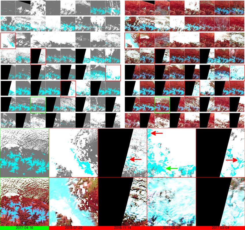
494                                                                                   S. Gascoin et al.: Theia Snow collection

which should be achieved using Earth observation satellites       and freely distributed via the Theia land data centre.1 The
in the near future (2018–2022).                                   snow retrieval algorithm is based on the Normalized Differ-
   Operational SCA maps have been generated from satellite        ence Snow Index (Dozier, 1989) but also uses a digital ele-
observations since the 1960s (Ramsay, 1998). Current SCA          vation model to better constrain the snow detection. We first
and fSCA products are mostly derived from MODIS data              describe the algorithm (Sect. 2) and its implementation in the
(Hall et al., 2002; Sirguey et al., 2008; Painter et al., 2009;   let-it-snow processor (LIS, Sect. 2.4.4). Then, we provide a
Metsämäki et al., 2015), but their spatial resolution (1 km to    detailed description of the product characteristics (coverage,
250 m) can be too coarse for various applications, especially     period, format, etc.; Sect. 3). In Sect. 4, we present an evalu-
in mountain regions where the snow cover properties vary on       ation of Theia snow products using in situ snow depth mea-
scales of 10 to 100 m (Blöschl, 1999). High-resolution (30 m)     surements, very high-resolution clear-sky snow maps and vi-
snow cover maps can be generated from Landsat images but          sual control. We finally discuss the main limitations and po-
the low temporal revisit of the Landsat mission (16 d) is an      tential applications of the Theia Snow collection.
important limitation for snow cover monitoring, especially
considering that the cloud probability can exceed 50 % in         2     Algorithm
temperate mountains (Parajka and Blöschl, 2008; Gascoin
et al., 2015). Since 2017, with the launch of Sentinel-2B, the    2.1    Scope
Copernicus Sentinel-2 mission offers the unique opportunity
to map the snow cover extent at 20 m resolution with a re-        An algorithm was designed to determine the snow presence
visit time of 5 d (cloud permitting) (Drusch et al., 2012). The   or absence from Sentinel-2 and Landsat-8 observations out-
combination of Sentinel-2 and Landsat-8 data provides the         side areas of dense forest with the following requirements:
opportunity for even more frequent observations of the snow
                                                                      – It should be scalable, i.e. allow the processing of large
cover with a global median average revisit interval of 2.9 d
                                                                        areas (104 km2 ) with a reasonable computation cost
(Li and Roy, 2017).
                                                                        (typically less than 1 h for a single product).
   The principles of snow detection from multispectral op-
tical imagery is well established since the pioneering work           – It should be robust to seasonal and spatial variability of
of Dozier (1989) with the Landsat Thematic Mapper. Today,               the snow cover and land surface properties.
the challenge for scientists and end users is rather to cope
with the large amount of data that is generated by a mission          – It should maximize the number of pixels that are classi-
like Sentinel-2. The generation of a single snow map from               fied as snow or no snow.
a Sentinel-2 level-1C tiled product (monodate orthorectified
                                                                      – It is preferable to falsely classify a pixel as cloud than
image expressed in top-of-atmosphere reflectance) involves
                                                                        falsely classify a pixel as snow or no snow.
downloading a 700+ Mb zip file (once uncompressed, the
product contains 12 folders and 108 files, including 15 raster
files and 13 XML metadata files). Since March 2018, ESA           2.2    Input
began the operational processing of level 2A (L2A) prod-          The algorithm works with multispectral remotely sensed im-
ucts (monodate orthorectified images expressed in surface         ages, which include at least a channel in the visible part
reflectance, including a cloud mask). Each ESA L2A prod-          of the spectrum and a channel near 1.5 µm (referred to as
uct also includes a snow cover mask. However, the size of         shortwave-infrared or SWIR). It takes the following as input:
a single L2A product before unzipping can exceed 1 Gb (15
folders, 137 files). In addition, the quality of the ESA L2A          – a L2A product, including
snow mask can be improved for two reasons: (i) ESA’s L2A
algorithm is a general-purpose algorithm, which was not op-               – the cloud and cloud shadow mask (referred to as an
timized for snow detection, and (ii) because ESA’s L2A pro-                 “L2A cloud mask” in the following),
cessor treats each image independently (i.e. mono-date ap-                – the green, red and SWIR bands from the flat-surface
proach, Louis et al., 2016), the output cloud mask has a lower              reflectance product. These images are corrected
accuracy than a cloud mask generated by a multi-temporal                    for atmospheric and terrain slope effects (Hagolle
algorithm (Hagolle et al., 2010).                                           et al., 2017). The slope correction is important in
   In this article we introduce the Theia Snow collection, a                mountain regions since it enables us to use the same
new collection of snow cover maps, which are derived from                   detection thresholds whatever the sun-slope geom-
Sentinel-2 at 20 m resolution in an operational context. The                etry.
Theia Snow collection was recently upgraded to also provide
snow cover maps at 30 m resolution from Landsat-8 using               – A digital elevation model (DEM).
the same algorithm. The data are currently being produced            1 Theia is a French inter-agency organization designed to foster
                                                                  the use of Earth observation for land surface monitoring for aca-
                                                                  demics and public policy actors.

Earth Syst. Sci. Data, 11, 493–514, 2019                                            www.earth-syst-sci-data.net/11/493/2019/
S. Gascoin et al.: Theia Snow collection                                                                                       495

2.3     Pre-processing                                              pixels is not considered statistically significant for determin-
                                                                    ing the snow line elevation. Otherwise, the pass 2 is activated.
The red and green bands are resampled with the cubic
                                                                    For that purpose, the DEM is used to segment the image in
method to a pixel size of 20 m by 20 m to match the resolu-
                                                                    elevation bands with a fixed height of dz (Table 1). Then,
tion of the SWIR band. The DEM is generated from the Shut-
                                                                    the fraction of the cloud-free area that is covered by snow
tle Radar Topography Mission seamless DEM (Jarvis et al.,
                                                                    in each band (after pass 1) is computed. The algorithm finds
2008) by cubic spline resampling to the same 20 m resolution
                                                                    the lowest elevation band b at which the snow cover fraction
grid.
                                                                    is greater than a given fraction fs (Table 1). The value of zs
                                                                    is the lower edge of the elevation band that is two elevation
2.4     Algorithm description                                       bands below band b.
2.4.1    Snow detection
                                                                    2.4.3   Cloud mask processing
The snow detection is based on the Normalized Difference
Snow Index (NDSI, Dozier, 1989) and the reflectance in the          The cloud mask in the input L2A product is conservative
red band. The NDSI is defined as                                    because (i) it is computed at a coarser resolution and (ii) it
                                                                    was developed to remove surface reflectance variations due
           ρgreen − ρSWIR
NDSI =                    ,                                  (1)    to cloud contamination. However, the scattering of some thin
           ρgreen + ρSWIR                                           clouds is low in the SWIR, green and red bands, which are
                                                                    used for snow detection (Sect. 2.4.1). Hence, the human eye
where ρgreen (or ρSWIR ) is the slope-corrected surface re-
                                                                    can see the snow (or the absence thereof) through these semi-
flectance in the green band (or SWIR at 1.6 µm). The NDSI
                                                                    transparent clouds in a colour composite. In addition, the
expresses the fact that only snow surfaces are very bright
                                                                    L2A cloud mask tends to falsely classify the edges of the
in the visible and very dark in the shortwave infrared. Tur-
                                                                    snow cover as cloud. Therefore, the algorithm includes some
bid water surfaces like some lakes or rivers may also have
                                                                    additional steps to recover those pixels from the L2A cloud
a high NDSI value; hence a additional criterion on the red
                                                                    mask and reclassify them as snow or no snow. This step is
reflectance is used to avoid false snow detection in these ar-
                                                                    important because it substantially increases the number of
eas. A cloud-free pixel is classified as snow if the following
                                                                    observations as specified in Sect. 2.1.
condition is true:
                                                                       A pixel from the L2A cloud mask cannot be reclassified as
(NDSI > ni ) and (ρred > ri ) ,                              (2)    snow or no snow if any of these conditions are satisfied:

                                                                      – it is coded as “cloud shadow” in the L2A cloud mask;
where ni and ri are two parameter pairs (i.e. i ∈ {1, 2}) as ex-
plained below. Otherwise the pixel is marked as “no snow”.            – it is coded as “high-altitude cloud” (or “cirrus”) in the
The values of the parameters are provided in Table 1.                   L2A cloud mask;

2.4.2    Snow line elevation                                          – it is not a “dark cloud” (see below).

The algorithm works in two passes. The snow detection                  The cloud shadows are excluded because the signal-to-
(Sect. 2.4.1) is performed a first time using parameters n1 and     noise ratio can be very low in these areas. The high clouds
r1 , which are set in such way as to minimize the number of         are excluded because they can have a similar spectral signa-
false snow detections (Table 1). This first pass enables us to      ture as the snow cover, i.e. a high reflectance in the visible
estimate the minimum elevation of the snow cover zs , above         and a low reflectance in the SWIR. This type of cloud are
which a second pass will be performed with less conserva-           detected in Sentinel-2 and Landsat-8 L2A products based on
tive parameters values n2 and r2 (Table 1). An example of           the spectral band centred on the 1.38 µm wavelength (Gao
the evolution of the snow line elevation over the tile 31TCH        et al., 1993).
in the Pyrenees is shown in Fig. 1 and the corresponding               We select only the dark clouds as possible reclassifica-
snow maps are shown in Fig. 1. Based on regional analy-             tion areas, because the NDSI test is robust to the snow–
ses of the snow line elevation variability in mountain ranges,      cloud confusion in this case. The dark clouds are defined us-
(e.g. Gascoin et al., 2015; Krajčí et al., 2016), we assume that   ing a threshold in the red band after downsampling the red
large altitudinal variations of the snow line elevation are not     band by a factor rf using the bilinear method. This resam-
likely on the scale of a tile of 110 km by 110 km. Therefore,       pling is applied to smooth locally anomalous pixels, follow-
the minimum snow elevation zs is considered uniform on the          ing the MAJA algorithm, which performs the cloud detection
scale of the processed image.                                       at 240 m for L2A products (Hagolle et al., 2017). Therefore,
    Before proceeding to pass 2, the total snow fraction in the     if a (non-shadow, non-high-cloud) cloud pixel has a red re-
image after pass 1 is computed. If this snow fraction is below      flectance at this coarser resolution that is lower than rD (Ta-
ft (Table 1), then pass 2 is skipped, as the sample of snow         ble 1), then it is temporarily removed from the cloud mask

www.earth-syst-sci-data.net/11/493/2019/                                              Earth Syst. Sci. Data, 11, 493–514, 2019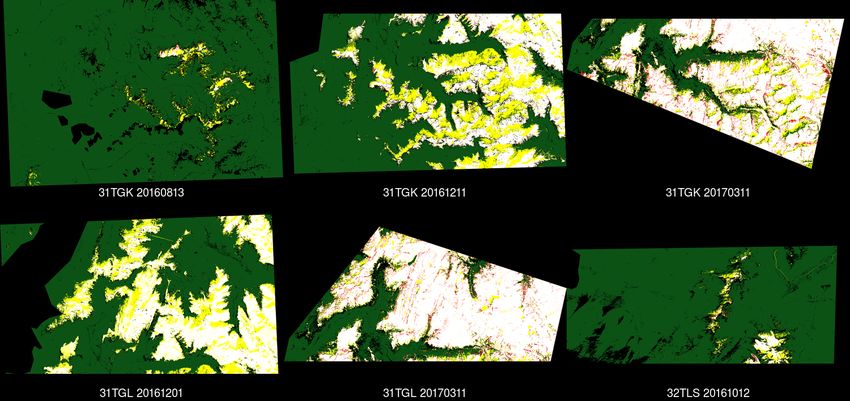
496                                                                                         S. Gascoin et al.: Theia Snow collection

Figure 1. Time series of snow and cloud cover area distribution by elevation band over tile 31TCH (tile location in Fig. 5). The dashed red
line indicates the position of zs as determined by the LIS algorithm. The corresponding snow maps are shown in Fig. 2.

Figure 2. Time series of snow maps over tile 31TCH (tile location in Fig. 5). The corresponding charts of snow and cloud cover area
distribution by elevation band are shown in Fig. 1.

Earth Syst. Sci. Data, 11, 493–514, 2019                                                  www.earth-syst-sci-data.net/11/493/2019/

S. Gascoin et al.: Theia Snow collection                                                                                     497

and proceeds to the pass 1 snow detection. The new cloud          rope (France, Spain, Switzerland, Italy, western Austria).
mask at this stage is the pass 1 cloud mask in Fig. 3.            The snow products are also provided for southern Quebec in
   After passing the passes 1 and 2, some former cloud pix-       Canada, the Issyk-Kul lake catchment in Kyrgyzstan and the
els (pixels that were originally marked as cloud in the L2A       Kerguelen Islands. These extra-European sites were selected
cloud mask) will not be reclassified as snow because they did     to support specific ongoing projects in relation with Theia.
not fulfil the conditions of Eq. (2). These pixels are flagged    An opportunistic tile is produced in central Nevada, USA,
as cloud in the final snow product if they have a reflectance     because this tile is already available as a level-2A version
in the red that is greater than rB (Table 1). Otherwise they      for calibration purposes. The Theia Snow collection covers
are classified as no snow. Here, the red band at 20 m resolu-     a number of mountain ranges with seasonal snow cover (Ta-
tion is used to allow an accurate detection of the snow-free      ble 3).
areas near the snow cover edges that the L2A product tend to         The Theia Snow collection products are available for 127
falsely mark as cloud. The resulting cloud mask is the pass 2     tiles, starting on December 2017. At the time of writing there
cloud mask in Fig. 3.                                             were over 17 000 available products. A set of 1300 products
                                                                  tagged as version 1.0 are available between November 2015
2.4.4   Implementation                                            and June 2017 for a subset of 15 tiles (Table 3). These prod-
                                                                  ucts were produced in pre-operational using a different con-
The algorithm was implemented in an open-source processor         figuration of LIS, which underestimated the snow-covered
called let-it-snow (LIS). LIS is written in Python 2.7 and C++    area on shaded slopes. All other products were generated
and relies on the Orfeo ToolBox and GDAL libraries. GDAL          with the same configuration as presented in this article. The
is used for input and output operations, image resampling         products after December 2017 can still have a different ver-
and metadata access (GDAL/OGR contributors, 2018). Or-            sion tag because of changing versions in the upstream L2A
feo Toolbox enables us to make the computations with good         product. However, the different L2A versions have a low
performances under memory constraints (i.e. the amount of         impact on the snow products. It is expected that the cloud
available memory can be predefined), which is critical for        mask has improved gradually with time, due to algorithms
operational production (Grizonnet et al., 2017). LIS takes        enhancements in the successive L2A versions and also be-
as input a digital elevation model and a Theia L2A prod-          cause of the increasing revisit frequency of the Sentinel-2
uct from Sentinel-2 MSI, Landsat-8 OLI, SPOT-4 HRVIR or           mission (the full 5 d revisit became nominal above all land
SPOT-5 HRG (Gascoin et al., 2018). The spatial resolution         masses in March 2018). The different versions of the Theia
and central wavelength of the spectral bands used by LIS for      Snow collection are listed and updated on this page: http://
each sensor are given in Table 2. It is also compatible with      www.cesbio.ups-tlse.fr/multitemp/?page_id=13180 (last ac-
Landsat-8 USGS level 2 products (U.S. Geological Survey           cess: 12 April 2019).
Earth Resources Observation And Science Center, 2014) and            The snow products are currently routinely generated at
Sentinel-2 ESA’s Sen2Cor level 2A products (Louis et al.,         CNES using the MUSCATE scheduler, which also manages
2016).                                                            the L2A production for Theia. MUSCATE performs a series
   The parameter values were set based on previous studies        of operations in a high-performance computing environment:
with Landsat (Hagolle et al., 2010; Zhu et al., 2015; Gascoin     (i) download the level 1C product as soon it is available from
et al., 2015) and by visually checking many snow maps and         the French mirror of the Sentinel products (PEPS, Plateforme
snow fraction histograms. From this set of a priori parameter     d’Exploitation des Produits Sentinel), (ii) process and dis-
values, only r2 was adjusted based on the analysis of a first     tribute the L2A product and (iii) process and distribute the
batch of products to enhance the snow detection on shaded         snow product. This workflow is optimized to reduce the lag
slopes.                                                           time between the acquisition and the distribution of the prod-
                                                                  ucts. As an example, in April 2018, nearly 80 % of the snow
3   Data description                                              products were made available online 5 d or less after the date
                                                                  of the Sentinel-2 acquisition (Fig. 6). It is expected that this
The Theia Snow collection data can be freely accessed us-         time lag should reach a median value of 2 d thanks to the
ing a web browser by connecting to http://theia.cnes.fr (last     increasing performance of MUSCATE.
access: 12 April 2019) or using this free command-line               Each snow product is distributed as a zipped file which
tool: https://github.com/olivierhagolle/theia_download (last      contains raster and vector files. The file base name is the
access: 12 April 2019). The user must first create an account     product ID, i.e. productId.zip, where the productId
in Theia to have the permission to download the data.             is a character string which is constructed as follows:
    The Theia Snow collection is organized following the
tiling system of Sentinel-2 (Fig. 4). Each tile covers a square   productId = Satellite_AcquisitionDate_
area of 110 km by 110 km in the UTM coordinate system.            _L2B-SNOW_TileName_D_Version.
There are currently 127 tiles in the Theia Snow collection,
mostly over the mountain ranges of western continental Eu-

www.earth-syst-sci-data.net/11/493/2019/                                            Earth Syst. Sci. Data, 11, 493–514, 2019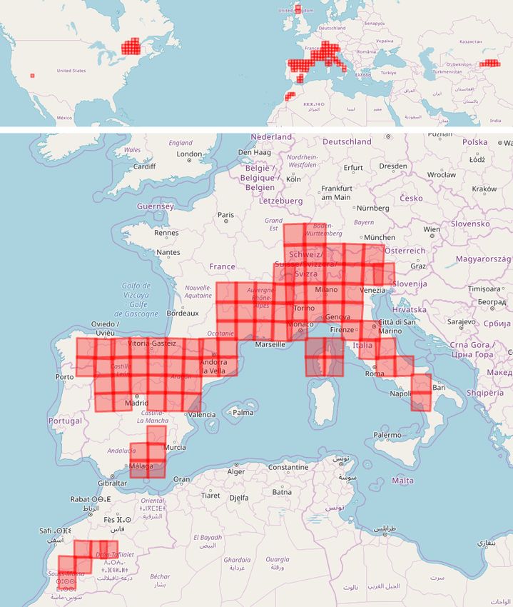
498                                                                                          S. Gascoin et al.: Theia Snow collection

Figure 3. Flow chart of the snow detection algorithm. Table 1 gives the description and value of the algorithm parameters (written in red in
this chart). MUSCATE is the scheduler which manages the L2A production for Theia.

For example, the eastern snow product in Fig. 5 was extracted           10:56:41.486 UTC and covers tile 31TDH. The version of
from a file named                                                       the product is 1.0 (see above).
                                                                           The size of each zipped product varies depending on the
SENTINEL2A_20151130-105641-486_L2B-
                                                                        complexity of the snow and cloud mask but generally ranges
-SNOW_T31TDH_D_V1-0.zip,                                                between 10 and 100 Mb. After extracting the product, the fol-
which indicates that this product was generated from a                  lowing files are created:
Sentinel-2A image acquired on 30 November 2015 at

Earth Syst. Sci. Data, 11, 493–514, 2019                                                   www.earth-syst-sci-data.net/11/493/2019/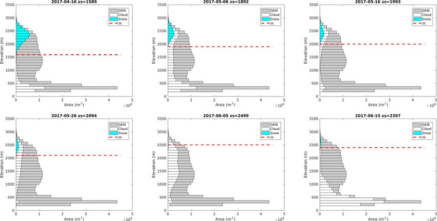
S. Gascoin et al.: Theia Snow collection                                                                                         499

Table 1. LIS algorithm parameters description and default values for Theia’s L2A Sentinel-2 (and Landsat-8) products.

            Parameter    Description                                                                                    Value
            rf           Resize factor to produce the downsampled red band                                              12 (8)
            rD           Maximum value of the downsampled red-band reflectance used to define a dark cloud pixel        0.300
            n1           Minimum value of the NDSI for the pass 1 snow test                                             0.400
            n2           Minimum value of the NDSI for the pass 2 snow test                                             0.150
            r1           Minimum value of the red-band reflectance the pass 1 snow test                                 0.200
            r2           Minimum value of the red-band reflectance the pass 2 snow test                                 0.040
            dz           Size of elevation band in the DEM used to define zs                                            100
            fs           Minimum snow fraction in an elevation band to define zs                                        0.100
            fct          Minimum clear pixels fraction (snow and no snow) in an elevation band used to define zs        0.100
            ft           Minimum snow fraction in the image to activate the pass 2 snow test                            0.001
            rB           Minimum value of the red band reflectance to return a non-snow pixel to the cloud mask         0.100

Figure 4. Coverage of the Theia Snow collection tiles.

www.earth-syst-sci-data.net/11/493/2019/                                                  Earth Syst. Sci. Data, 11, 493–514, 2019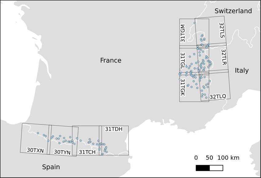
500                                                                                   S. Gascoin et al.: Theia Snow collection

Figure 5. Map of the first two products in the Theia Snow collection and comparison with MOD10A1.005 snow product of the same day.
The map background is the colourized version of the EU DEM.

Table 2. Spatial resolution and central wavelength of the spectral      which contains a vectorized version of the pro-
bands used by LIS for each compatible sensor.                           ductID_SNW_R2.tif using the polygon geometry.

 Sensor             Green band       Red band       SWIR band         – productID_CMP_R2.tif is an 8 bit RGB GeoTiff
 SPOT-4 HRV        20 m, 0.55 µm   20 m, 0.65 µm    20 m, 1.6 µm        image which shows the outlines of the snow mask
 SPOT-5 HRG        10 m, 0.55 µm   10 m, 0.65 µm    10 m, 1.6 µm        (green lines) and cloud mask (magenta lines) on a
 Sentinel-2 MSI    10 m, 0.56 µm   10 m, 0.66 µm    20 m, 1.6 µm        false-colour composite of the input L2A image (RGB
 Landsat-8 OLI     30 m, 0.56 µm   30 m, 0.65 µm    30 m, 1.6 µm        image made with SWIR, red and green bands). This
                                                                        composition was chosen because RGB composites us-
                                                                        ing the SWIR-band image are useful for discriminating
  – productID_SNW_R2.tif is an 8 bit single-band                        the snow cover from the snow-free areas and from the
    GeoTiff image which provides the following classifica-              clouds (Vidot et al., 2017). Hence, this image mainly
    tion for each pixel:                                                allows the user to visually check the consistency of the
                                                                        snow and cloud mask.
       – 0: no snow,
       – 100: snow,                                                   – productID_MTD_ALL.xml is a metadata file.
       – 205: cloud including cloud shadow,
       – 254: no data.                                                – productID_QKL_ALL.jpg is a quick picture of the
                                                                        productID_SNW_R2.tif image made using this
  – productID_SNW_R2.{shp,shx,dbf,prj}                                  colour map (8 bit RGB code in parentheses): snow
    is a vector file in the ESRI shapefile format,                      in cyan (0,255,255), cloud in white (255,255,255), no

Earth Syst. Sci. Data, 11, 493–514, 2019                                            www.earth-syst-sci-data.net/11/493/2019/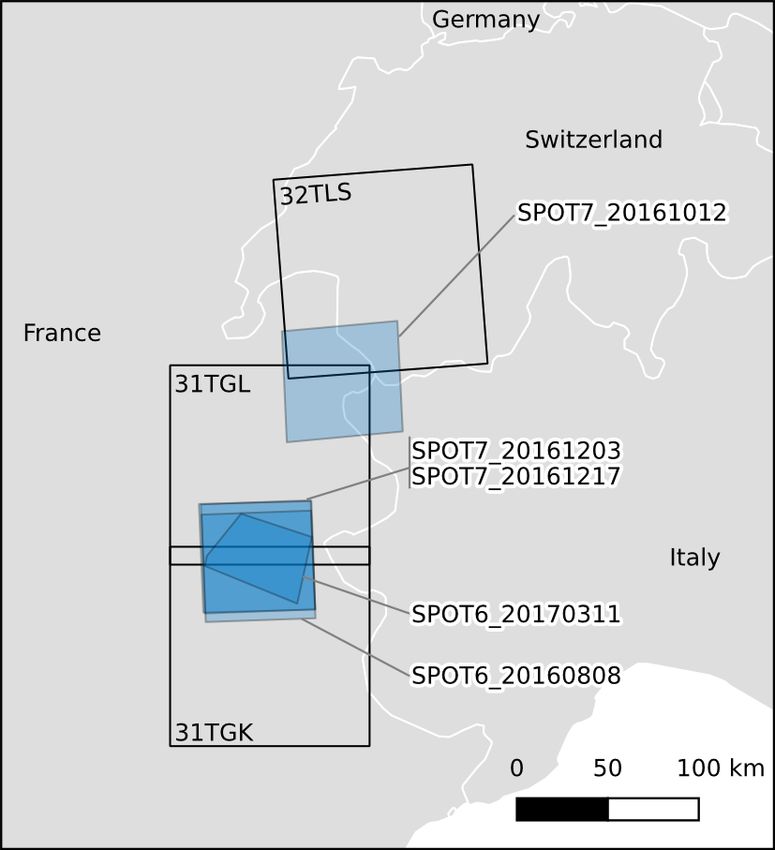
S. Gascoin et al.: Theia Snow collection                                                                                                                     501

Table 3. Non-exhaustive list of mountain ranges covered by the Theia Snow collection and corresponding tiles. The tiles marked with an
asterisk were made available before the start of the operational production (see Sect. 3).

               Mountain range             Tiles
               Alps                       32TMS, 32TMR, 32TMT, 32TNS, 32TNR, 32TLQ∗ , 32TLP, 32TLS∗ , 32TLR∗ , 32TQT,
                                          32TQS, 33TUM, 31TGK∗ , 32TNT, 31TGJ, 32TPR, 31TGL∗ , 32TPT, 32TPS
               Appenines                  33TUH, 32TNQ, 33TUG, 33TVG, 33TWF, 32TPP, 33TWE, 32TPQ, 32TQP, 32TQN
               Cantabrian                 30TUN, 29TPH, 29TPG, 29TQH
               Corsica                    32TMM, 32TMN, 32TNM, 32TNM
               Grant Range                11SPC
               High Atlas                 29RPQ∗ , 29RNQ∗ *, 29SQR∗ , 29SPR∗ , 30STA∗
               Sistema Iberico            30TVM, 30TWK, 30TWM, 30TWL, 30TXK, 30TXL
               Jura                       31TGM∗ , 32TLT
               Lebanon                    T36SYD, T37SBU, T36SYC, T37SBT, T36SYB
               Massif Central             31TDL,3 1TDK, 31TEK, 31TEL
               Pyrenees                   30TXN∗ , 30TYM, 30TYN∗ , 31TCG, 31TDG, 31TCH∗ , 31TDH∗
               Sierra de Cazorla          30SWH
               Sierra Nevada              30SVG, 30SWG
               Sistema Central            30TUL, 30TUK, 30TVL, 30TTK
               Vosges                     32TLT, 32ULU
             ∗ These tiles can be viewed on an interactive map on this page: https://theia.cnes.fr/atdistrib/rocket/\T1\textbackslash#/sites (last access:
             12 April 2019).

                                                                                                   bit indicates the value of an intermediate computation
                                                                                                   mask (Sect. 2):

                                                                                                      – bit 1: snow (pass 1),

                                                                                                      – bit 2: snow (pass 2),

                                                                                                      – bit 3: clouds (pass 1),

                                                                                                      – bit 4: clouds (pass 2),

                                                                                                      – bit 5: clouds (initial all cloud).

                                                                                           For most applications, only files with the SNW suffix should
                                                                                           be useful.
                                                                                              The shapefile and raster images are referenced in WGS-
                                                                                           84 UTM system with the zone number given by the first two
Figure 6. Cumulative probability of the time lags between the
Sentinel-2 acquisition and the distribution date of the correspond-
                                                                                           digits of the tile name. All raster files have a 20 m resolution.
ing snow product, computed for all snow products with acquisition                          Note that no-snow pixels can be any surface, including water
date in April 2018.                                                                        surface. No data pixels are the pixels outside of the acquisi-
                                                                                           tion segment.

     snow in grey (119,119,119) and no data in black (0,0,0)
     (see an example in Fig. 7).                                                           4     Evaluation

  – DATA/productID_HIS_R2.txt (since product                                               In this section we present an evaluation of the Theia Snow
    version 1.4) is a text file indicating the cloud, snow and                             collection. We first present the methods developed to do
    no-snow fraction area by elevation bins (Sect. 2).                                     this evaluation and then the results. The evaluation was
                                                                                           based only on Sentinel-2 products, because the production
  – MASKS/productID_EXS_R2.tif (in product ver-                                            for Landsat-8 had just started at the time of writing and thus
    sion 1.0, it is located in the root of the zipped file) is an                          the Landsat-8 products represented a very minor fraction of
    8 bit GeoTiff image for expert evaluation, where each                                  the Theia Snow collection.

www.earth-syst-sci-data.net/11/493/2019/                                                                             Earth Syst. Sci. Data, 11, 493–514, 2019
502 S. Gascoin et al.: Theia Snow collection
Figure 7. Example of a snow map (SNW file) and its corresponding colour composite (CMP file). In the snow map the snow is represented
in cyan, no snow in grey and cloud in white. In the RGB composite, the snow-covered areas are delineated in magenta, while the clouds are
delineated in green (Theia snow product of tile 32TNS on 27 May 2017).
4.1 Method products with ground measurements showed that a value of
0 m may not be optimal (Klein and Barnett, 2003; Gascoin
4.1.1 Comparison with in situ snow depth
et al., 2015); therefore the sensitivity of the results to SD0
measurements
was tested by recomputing the confusion matrix for 1 cm in-
We collected all available snow depth measurements within crements of SD0 from 0 to 1 m.
tiles 31TGM, 31TGL, 31TGK, 32TLS, 32TLR, 32TLQ,
31TDH, 31TCH, 30TYN and 30TNX from the Météo- 4.1.2 Comparison with snow maps of higher spatial
France database between 1 September 2017 and 31 August resolution
2018. These 10 tiles cover most of the French Alps and Pyre-
nees (Fig. 8). We obtained 120 snow depth time series with We used SPOT-6 and SPOT-7 images with a resolution of
at least one measurement. We gathered all available Sentinel- 1.5 m in panchromatic and 6 m in multispectral (blue, green,
2 snow products for these tiles over the same period, i.e. red, near-infrared) to evaluate the accuracy of the snow de-
a total of 1134 products. Then, we extracted the pixel val- tection in Theia snow products. For this comparison, the
ues at the location of each snow measurement station for all LIS processor was run with its current operational config-
dates. When a station is located in two tiles we only kept the uration (i.e. the configuration used to routinely produce the
data from the first tile. We selected the snow depth measure- Theia snow products since December 2017 Table 1). SPOT-
ments which were collected on the same day of a Theia snow 6 and SPOT-7 sensors acquire images with a large radio-
product and discarded the measurements corresponding to a metric depth coded in 16 bits, which enables us to identify
cloud detection in the Theia snow product. The snow depth surface features in alpine regions with dark shaded slopes
measurements were converted to snow presence and absence and bright snow surfaces. We searched the catalogue of the
using a threshold of SD0 = 0 m. This eventually allowed us Kalideos database for available SPOT images that could
to compute a confusion matrix between a set of snow pres- match a cloud-free (or nearly cloud-free) Theia snow map
ence and absence data from in situ measurement and a set over the French Alps region (https://alpes.kalideos.fr, last ac-
of simultaneous snow presence and absence data from the cess: 12 April 2019). We identified six pairs of images in
Theia Snow collection across the French Alps and Pyrenees. 2016 and 2017 with a maximum time lag of 6 d (Table 4,
However, previous studies comparing MODIS binary snow Fig. 9). The SPOT images were obtained as orthorectified
Earth Syst. Sci. Data, 11, 493–514, 2019 www.earth-syst-sci-data.net/11/493/2019/S. Gascoin et al.: Theia Snow collection 503
Figure 8. Map showing the location of the stations in the réseau nivo-météorologique (Météo-France snow observation network) used for
this study (source: Météo-France) and the corresponding Sentinel-2 tiles.
products from the Kalideos database. The SPOT images were Table 4. Pairs of Sentinel-2 and SPOT-6/7 products used for the
used to generate reference snow maps by a pixel-based su- evaluation of the snow detection accuracy (see also Fig. 9).
pervised classification. For each SPOT image, we manually
drew about 15 polygons of homogeneous of snow and no- Sentinel-2 product Reference product
snow surfaces using the panchromatic image. The few cloud Tile Date Sensor Date
pixels in the SPOT images were also manually delineated
with a large buffer to restrict the classification to strictly 31TGK 13 Aug 2016 SPOT-6 8 Aug 2016
cloud-free areas. Colour composites made from the multi- 32TLS 12 Oct 2016 SPOT-7 12 Oct 2016
31TGK 11 Dec 2016 SPOT-7 17 Dec 2016
spectral images were also used as a visual support to help
31TGL 1 Dec 2016 SPOT-7 3 Dec 2016
the snow and cloud classification. These polygons were then 31TGK 11 Mar 2017 SPOT-6 11 Mar 2017
used to extract training samples from the SPOT products. The 31TGL 11 Mar 2017 SPOT-6 11 Mar 2017
samples were taken from both the panchromatic and the mul-
tispectral images. We tested a number of classification algo-
rithms by splitting the polygons in calibration and validation
rics derived from the confusion matrix (accuracy, F1 score,
data sets. The detail of this analysis is not shown here, but it
kappa, false-detection rate and false-negative rate).
allowed us to conclude that the random forest classifier was
the best choice for our purpose, given its good accuracy and
its numerical efficiency (Bouchet, 2018). 4.1.3 Evaluation metrics
In addition, we generated the snow maps from the same From the confusion matrices of Sect. 4.1.1 and 4.1.2, we de-
Sentinel-2 level 1 products using ESA’s Sen2Cor version 2.5 rived the following metrics: accuracy (the proportion of the
(Louis et al., 2016). The Sen2Cor output snow masks are ex- total number of predictions that were correct), false-positive
pected to be nearly identical to the ones included in the dis- rate (FPR, i.e. the proportion of no-snow pixels that were in-
tributed L2A products by ESA, since the same processor is correctly classified as snow), false-negative rate (FNR, i.e.
used. We have generated the L2A products ourselves with the proportion of snow pixels that were incorrectly classified
Sen2Cor for this study, because the L2A products were not as no snow), F1 score (harmonic average of the precision and
yet available when we made this analysis (ESA started op- recall) and kappa coefficient (Cohen, 1960).
erational production of Sentinel-2 data at level 2A in 2017).
The Theia and Sen2Cor snow maps were compared to the
reference snow maps from SPOT images using standard met-
www.earth-syst-sci-data.net/11/493/2019/ Earth Syst. Sci. Data, 11, 493–514, 2019504 S. Gascoin et al.: Theia Snow collection
Table 5. Confusion matrix between the Theia snow products and in
situ snow depth data (SD).
Theia snow products
In situ snow depth no snow snow
SD = 0 276 8
SD > 0 76 1054
4.1.4 Visual verification
The evaluation methods presented above undersample the ac-
tual resolution of the Theia snow collection, both in space
(only 120 points of comparisons in Sect. 4.1.1) and time
(only six dates of comparisons in Sect. 4.1.2). Given that we
do not have a more extensive validation data set, we used a
time series of 64 Theia snow products from 6 July 2015 to
2 July 2017 over tile 31TCH to control the consistency of the
snow and cloud masks based on the visual inspection of the
false-colour composites. This approach is efficient for evalu-
ating the frequency of gross errors on the tile scale, i.e. large
patches of false snow or false no-snow detection (Vidot et al.,
2017).
4.2 Results
Figure 9. Location of the five SPOT-6/7 products used for the
4.2.1 Comparison with in situ snow depth
evaluation of the snow detection accuracy and the corresponding
measurements Sentinel-2 tiles (see also Table 4).
The confusion matrix between the Theia snow products and
in situ snow depth measurements is given in Table 5. We find
1414 pairs of data for the study period (i.e. there are 1414
individual snow depth measurements for which a cloud-free
retrieval can be found in the Theia Snow collection on the
same day). From this confusion matrix, the accuracy (pro-
portion of correct classifications) is 94 % and the kappa co-
efficient is 0.83, which indicates excellent agreement accord-
ing to Fleiss et al. (2013). The false-positive rate (2.8 %) is
lower than the false-negative rate (6.7 %), which means that
the Theia snow product is more likely to underestimate than
to overestimate the snow detection at the station locations.
The false-negative rate decreases if SD0 is set to a higher
value; however the false-positive rate also increases in such
a way that an optimum is reached at SD0 = 2 cm (Fig. 10).
The comparisons of each individual time series before
matching the data by date is shown in Appendix B. These
plots illustrate that the high revisit time of Sentinel-2 enables
us to capture the seasonal cycle of the snow cover well. Even
intermediate melt-out events at lower elevation stations can
be identified over the course of the snow season.
Figure 10. Sensitivity of the agreement between the in situ and
Theia snow product to SD0 in metres (threshold to convert the mea-
4.2.2 Comparison with snow maps of higher spatial sured snow depth to snow presence or absence). The inset shows a
resolution close-up of the region of 0–0.2 m.
Table 6 shows that the MAJA–LIS workflow provides a bet-
ter detection of the snow cover than the Sen2Cor processor in
Earth Syst. Sci. Data, 11, 493–514, 2019 www.earth-syst-sci-data.net/11/493/2019/S. Gascoin et al.: Theia Snow collection 505
Table 6. Results of the validation of Theia (LIS 1.2.1) and ESA (Sen2Cor 2.5) snow products using SPOT-6/7 reference snow maps.
Sentinel-2 product Accuracy F1 Kappa FPR FNR
Tile Date Sen2Cor LIS Sen2Cor LIS Sen2Cor LIS Sen2Cor LIS Sen2Cor LIS
31TGK 11 Dec 2016 0.83 0.92 0.73 0.91 0.61 0.84 0.41 0.04 0.05 0.14
31TGL 11 Mar 2017 0.89 0.90 0.92 0.93 0.74 0.76 0.09 0.02 0.06 0.11
31TGL 1 Dec 2016 0.84 0.95 0.78 0.95 0.66 0.90 0.35 0.05 0.01 0.06
31TGK 11 Mar 2017 0.85 0.89 0.89 0.92 0.65 0.72 0.15 0.01 0.07 0.13
31TGK 13 Aug 2016 0.98 0.99 0.35 0.77 0.34 0.77 0.78 0.24 0.22 0.22
32TLS 12 Oct 2016 0.98 0.97 0.63 0.64 0.62 0.62 0.49 0.08 0.17 0.51
all the studied cases. Although the improvement in the accu- which is close to 11 m at 95 % for both satellites accord-
racy coefficient is low in some cases (31TGL/2017-03-11, ing to the latest Sentinel-2 L1C data quality report (MPC
31TGK/2016-08-13) or even slightly negative in one case Team, 2018). In addition, in situ measurements may not be
(32TLS/2016-10-12), the F1 score and kappa coefficient of representative of the snow conditions within the Sentinel-2
the Theia snow products are always greater than or equal to pixel. However, the sensitivity analysis of the accuracy and
those of Sen2Cor. The differences are significant for four kappa coefficient to the SD0 value suggests that the discrep-
products among the six tested. The lower accuracy in the ancy between the scale of the in situ observations and the
case of the 32TLS/2016-10-12 product is due to a higher scale of the pixel observation is not significant, since the op-
false-negative rate. The false-positive rates in the Theia snow timal SD0 is close to 0 m. In contrast, a similar analysis with
products are generally lower than the false-negative rates, lower-resolution snow products from MODIS found an op-
which is consistent with the previous evaluation using in timal SD0 of 0.15 m Gascoin et al. (2015). This illustrates
situ data. The spatial analysis of the errors indicates that how high-resolution snow products from Sentinel-2 enable
the false-positives (i.e. overdetection of snow pixels) in the us to partly resolve the typical scale issue between in situ
Theia products are mostly located near the snow cover edges and remote-sensing products (Blöschl, 1999).
(Fig. A1). This suggests that these errors might not be due The visual inspection of the products reveals that the main
to a false detection of snow (e.g. confusion with a lake or a issue in some Theia snow products is rather the occurrence
cloud surface) but are rather due to the resolution discrepancy of false positives due to the confusion with cloud surfaces.
with the reference data. By contrast, the spatial comparison This problem can be due to two main factors:
of the Sen2Cor products with the reference data shows large
– Cold clouds: cold clouds have a spectral signature that
patches of false negatives (omission of snow pixels) in the
is close to the snow cover since they contain ice crys-
snow-covered area, which are typically due to the omission
tals (high NDSI). If these clouds are not accurately de-
of snow pixels in shaded areas (Fig. A2).
tected by the level 2A processor then the LIS algorithm
will also classify them as snow after pass 1 (Sect. 2).
4.2.3 Visual verification As a result the snow line elevation zs is not well es-
timated, which can generate erroneous snow patches
We found 4 products among 64 with significant patches of
within these clouds, even at low elevation (e.g. product
false-positive pixels (i.e. pixels falsely classified as snow).
of 20 July 2017 in Fig. 11).
These false snow areas are exclusively located in cloud areas
(Fig. 11). False-negative pixels (i.e. pixels falsely classified – Shaded clouds: the three-dimensional structure of the
as snow-free) can be found by looking at higher-resolution clouds can form shadows within the cloud cover area
data along the snow cover edges, but we did not find large (e.g. product of 4 March 2017 in Fig. 11). These shaded
areas of false-negative pixels. cloud areas have a lower reflectance in the visible wave-
lengths and therefore can be considered as dark clouds
in the LIS algorithm, provided that the shaded cloud
5 Discussion
cover area is large enough to significantly reduce the re-
flectance in the red band, even after the downsampling
The evaluation of the Theia Snow collection using both in
step (Sect. 2).
situ and remote-sensing reference data sets indicates an ex-
cellent accuracy of the snow detection, albeit with a tendency Among 64 products, we find 4 cases with significant false
to snow underdetection. The omission of snow pixels can be snow cover detection in this tile (Fig. 11). Although it is not
due to the presence of trees or shadows. In the case of the shown here, we have made this exercise over other tiles in the
in situ comparison, part of the errors may be explained by Alps and Atlas mountains, and we estimate that this propor-
the uncertainty in the geolocalization of the Sentinel-2 data, tion is similar in these areas. Regarding this issue we mainly
www.earth-syst-sci-data.net/11/493/2019/ Earth Syst. Sci. Data, 11, 493–514, 2019506 S. Gascoin et al.: Theia Snow collection Figure 11. Full time series of Theia snow products from 6 July 2015 to 2 July 2017 over tile 31TCH. Four products with visually evident false snow detections are framed in red and shown at higher resolution. Red arrows indicate the location of the false snow patches, while the green arrow indicates a true snow patch. The product of 16 April 2017 is shown as a reference to help the visualization of the errors. rely on our visual judgment using colour composites to as- detection in Sen2Cor, which can cause snow–cloud confu- sess the ability of the algorithm to discriminate the cloud sion in the L2A product, while LIS uses L2A products from and the snow cover. However, to further quantify the algo- the more accurate multi-temporal MAJA processor (Baetens rithm performance and eventually optimize its parameters, et al., 2019). In addition, a unique feature of the LIS algo- we would need a database of classified imagery with labelled rithm is the use of the snow line elevation concept to im- regions of cloud and snow cover in many different cases. prove the robustness of the snow detection in mountain re- Both Sen2Cor and LIS use the NDSI to detect the snow gions. In addition, LIS was designed to retrieve snow below cover; however the algorithms differ in many aspects. The thin clouds and to reclassify snow pixels which are frequently better performances of LIS in Sect. 4.2.2 can be related to the found near the snow cover edges in L2A products. Apart mono-date approach for atmospheric correction and cloud Earth Syst. Sci. Data, 11, 493–514, 2019 www.earth-syst-sci-data.net/11/493/2019/
S. Gascoin et al.: Theia Snow collection                                                                                       507

from the MAJA processing, however, the effect of these al-            The Theia Snow collection is based on optical observa-
gorithmic differences could be less evident in flat areas.         tions; therefore it is not adapted to the detection of the snow
                                                                   cover in dense forest areas where the ground is obstructed
                                                                   by the canopy (Xin et al., 2012). This may typically occur in
6   Code and data availability
                                                                   evergreen conifer forests of alpine regions (e.g. Alps, Pyre-
                                                                   nees). We have noted that the snow detection can be success-
The Theia snow collection can be accessed
                                                                   ful even in alpine forests, but we lack data that can be used for
and cited using this digital object identifier:
                                                                   quantifying its accuracy. Therefore it is recommended to use
https://doi.org/10.24400/329360/F7Q52MNK            (Gascoin
                                                                   a land cover map to exclude these forest areas from the anal-
et al., 2018). The let-it-snow source code is available
                                                                   ysis. For the tiles in France, this can be done using the Theia
under the GNU Affero General Public License v3.0 in this
                                                                   land cover map (Inglada et al., 2017), which is distributed at
repository: https://gitlab.orfeo-toolbox.org/remote_modules/
                                                                   the same spatial resolution. In the Pyrenees, the mean alti-
let-it-snow/ (last access: 12 April 2019).
                                                                   tude of zero-degree isotherm in winter is close to the treeline
                                                                   elevation at 1600 m; therefore the impact of the forest cover
7   Conclusions                                                    is limited (Gascoin et al., 2015). The LIS algorithm may also
                                                                   fail to detect the snow cover on steep, shaded slopes if the
The Theia Snow collection is a free collection of snow prod-       solar elevation is very low (typically below 20◦ ). This can
ucts which indicate the presence or absence of snow on             occur in midlatitude areas in winter. In this case, the slope
the land based on Sentinel-2 (20 m) and Landsat-8 (30 m)           correction in the L2A product is generally not applied. This
data. Most of the snow products are derived from Sentinel-         is indicated in the L2A mask but not in the snow product. A
2. However, in late September 2018, Landsat-8 snow prod-           future release of the Theia Snow collection should include
ucts started being routinely added to the Theia Snow col-          this information. However, the visual inspection of many im-
lection for the titles in France only. Previous Landsat-8 data     ages in regions of complex topography gives us the impres-
were also reprocessed back to March 2017. At the time of           sion that the snow detection algorithm already performs well
writing (15 March 2019), for example in tile T31TCH in             on shaded slopes. We are planning to investigate this issue
the Pyrenees, 20.5 % of all available products were derived        further using alternative approaches (Sirguey et al., 2009).
from Landsat-8 data (63 among 244). In addition, the pro-             In spite of all these limitations, the Theia snow products
cessing is done to facilitate the combination of Landsat-8         have already been successfully used for the evaluation of the
and Sentinel-2 snow products, since the data format and the        MODIS snow products (Masson et al., 2018) and the assim-
tiling scheme are the same (only the pixel size differs). Al-      ilation of snow-covered area data into a snowpack model in
though the co-registration of Sentinel-2 and Landsat-8 data        the High Atlas (Baba et al., 2018). Given that the snow cover
can be still problematic (Storey et al., 2016), the combination    is a key driver of many natural processes in mountains re-
of “analysis ready” Landsat-8 and Sentinel-2 is important for      gions, we envision various potential applications of the Theia
increasing the number of cloud-free observations.                  snow products, including the modelling of the distribution of
    The evaluation presented in this article indicate that the     the permafrost in mountain regions, the validation and cal-
Theia Snow product allows an accurate detection of the snow        ibration of hydrological models in snow-dominated catch-
cover (and of the absence of snow). However, it remains a          ments and the spatial modelling of biodiversity and produc-
preliminary assessment that should be extended in the fu-          tivity of ecosystems in mountain regions.
ture. For example, the evaluation was based only on Sentinel-
2 products, since the integration of Landsat-8 data started
during the writing of this paper and should be extended to
Landsat-8 products. However, the processing is done with
the same algorithm, which is based on the calculation of
the NDSI from slope-corrected surface reflectance (level 2A
data). In addition, the evaluation was limited to the French
Alps and French Pyrenees, while the collection covers other
mountain regions. Last, the spatial evaluation using higher-
resolution remote-sensing data was focused on the accuracy
of the snow detection using very high-resolution clear-sky
images, while, as discussed above, the main difficulty is not
to detect the snow when the sky is cloud-free but rather to
avoid false snow detection within clouds. The reduction of
the false-positive rate is the main challenge for the future de-
velopments in the LIS algorithm. In the meantime, we also
welcome feedback from other users.

www.earth-syst-sci-data.net/11/493/2019/                                             Earth Syst. Sci. Data, 11, 493–514, 2019
508 S. Gascoin et al.: Theia Snow collection Appendix A: Spatial comparison between Theia and Sen2Cor snow products with SPOT-6/7 reference data Figure A1. Theia snow products vs. SPOT-6/7 snow maps (green: true negative, white: true positive, red: false positive, yellow: false negative). Figure A2. Sen2cor snow product vs. SPOT-6/7 snow maps (green: true negative, white: true positive, red: false positive, yellow: false negative). Earth Syst. Sci. Data, 11, 493–514, 2019 www.earth-syst-sci-data.net/11/493/2019/
S. Gascoin et al.: Theia Snow collection                                                                                      509

Appendix B: Time series of Theia snow products and
snow depth records at 120 snow observation stations
from 1 September 2017 to 31 August 2018

Figure B1. Magenta dots: snow presence (a) or absence (b) in the Theia snow collection. Black line: snow depth time series.

www.earth-syst-sci-data.net/11/493/2019/                                                  Earth Syst. Sci. Data, 11, 493–514, 2019
510                                                                                        S. Gascoin et al.: Theia Snow collection

Figure B2. Magenta dots: snow presence (a) or absence (b) in the Theia snow collection. Black line: snow depth time series.

Earth Syst. Sci. Data, 11, 493–514, 2019                                                 www.earth-syst-sci-data.net/11/493/2019/
S. Gascoin et al.: Theia Snow collection                                                                                      511

Figure B3. Magenta dots: snow presence (a) or absence (b) in the Theia snow collection. Black line: snow depth time series.

www.earth-syst-sci-data.net/11/493/2019/                                                  Earth Syst. Sci. Data, 11, 493–514, 2019
512                                                                                        S. Gascoin et al.: Theia Snow collection

Figure B4. Magenta dots: snow presence (a) or absence (b) in the Theia snow collection. Black line: snow depth time series.

Earth Syst. Sci. Data, 11, 493–514, 2019                                                 www.earth-syst-sci-data.net/11/493/2019/
S. Gascoin et al.: Theia Snow collection                                                                                                  513

Author contributions. SG and OH defined the LIS algorithm.             Fleiss, J. L., Levin, B., and Paik, M. C.: Statistical methods for rates
MG and GS worked on the implementation and development of the             and proportions, John Wiley & Sons, 2013.
LIS processor. MG, MB and SG worked on the validation of the           Frei, A., Tedesco, M., Lee, S., Foster, J., Hall, D., Kelly,
snow products. SG wrote the manuscript with inputs from all the           R., and Robinson, D. A.: A review of global satellite-
co-authors.                                                               derived snow products, Adv. Space Res., 50, 1007–1029,
                                                                          https://doi.org/10.1016/j.asr.2011.12.021, 2012.
                                                                       Gao, B.-C., Goetz, A. F., and Wiscombe, W. J.: Cirrus cloud detec-
Competing interests. The authors declare that they have no con-           tion from airborne imaging spectrometer data using the 1.38 µm
flict of interest.                                                        water vapor band, Geophys. Res. Lett., 20, 301–304, 1993.
                                                                       Gascoin, S., Hagolle, O., Huc, M., Jarlan, L., Dejoux, J.-F.,
                                                                          Szczypta, C., Marti, R., and Sánchez, R.: A snow cover climatol-
Acknowledgements. The development and production of the                   ogy for the Pyrenees from MODIS snow products, Hydrol. Earth
Theia Snow collection is supported by the CNES. We thank Tris-            Syst. Sci., 19, 2337–2351, https://doi.org/10.5194/hess-19-2337-
tan Klempka for his contribution to earlier developments of the LIS       2015, 2015.
processor. We thank Marc Leroy, Arnaud Sellé and Philippe Pachol-      Gascoin, S., Grizonnet, M., Klempka, T., and Salgues, G.: Algo-
czyk for the coordination of the Theia project and Joelle Donadieu        rithm theoretical basis documentation for an operational snow
and Céline l’Helguen for the transfer to the production at MUS-           cover product from Sentinel-2 and Landsat-8 data (Let-it-snow),
CATE. This manuscript was greatly improved thanks to the con-             https://doi.org/10.5281/zenodo.1414452, 2018.
structive comments of Gaia Piazzi, Javier Herrero, Jeff Dozier and     Gascoin, S., Grizonnet, M., Hagolle, O., and Salgues, G.:
an anonymous referee.                                                     Theia Snow collection, CNES for THEIA Land data center,
                                                                          https://doi.org/10.24400/329360/f7q52mnk, 2018.
                                                                       GDAL/OGR contributors: GDAL/OGR Geospatial Data Abstrac-
                                                                          tion software Library, Open Source Geospatial Foundation, http:
Review statement. This    paper was edited by Alexander
                                                                          //gdal.org (last access: 12 April 2019), 2018.
Kokhanovsky and reviewed by Gaia Piazzi, Javier Herrero, Jeff
                                                                       Grizonnet, M., Michel, J., Poughon, V., Inglada, J., Savinaud, M.,
Dozier, and one anonymous referee.
                                                                          and Cresson, R.: Orfeo ToolBox: open source processing of re-
                                                                          mote sensing images, Open Geospatial Data, Software and Stan-
                                                                          dards, 2, 15, https://doi.org/10.1186/s40965-017-0031-6, 2017.
                                                                       Hagolle, O., Huc, M., Pascual, D. V., and Dedieu, G.: A multi-
References                                                                temporal method for cloud detection, applied to FORMOSAT-2,
                                                                          VENµS, LANDSAT and SENTINEL-2 images, Remote Sens.
Baba, M. W., Gascoin, S., and Hanich, L.: Assimilation of Sentinel-       Environ., 114, 1747–1755, 2010.
  2 Data into a Snowpack Model in the High Atlas of Morocco,           Hagolle, O., Huc, M., Desjardins, C., Auer, S., and Richter,
  Remote Sensing, 10, 1982, https://doi.org/10.3390/rs10121982,           R.: MAJA Algorithm Theoretical Basis Document,
  2018.                                                                   https://doi.org/10.5281/zenodo.1209633, 2017.
Baetens, L., Desjardins, C., and Hagolle, O.: Validation of Coper-     Hall, D., Riggs, G., Salomonson, V., DiGirolamo, N., and Bayr, K.:
  nicus Sentinel-2 Cloud Masks Obtained from MAJA, Sen2Cor,               MODIS snow-cover products, Remote Sens. Environ., 83, 181–
  and FMask Processors Using Reference Cloud Masks Generated              194, 2002.
  with a Supervised Active Learning Procedure, Remote Sensing,         Inglada, J., Vincent, A., Arias, M., Tardy, B., Morin, D., and Rodes,
  11, 433, https://doi.org/10.3390/rs11040433, 2019.                      I.: Operational High Resolution Land Cover Map Production at
Blöschl, G.: Scaling issues in snow hydrology, Hydrol. Process., 13,      the Country Scale Using Satellite Image Time Series, Remote
  2149–2175, 1999.                                                        Sensing, 9, 95, https://doi.org/10.3390/rs9010095, 2017.
Bouchet, M.: Validation et amélioration des pro-                       Jarvis, A., Guevara, E., Reuter, H. I., and Nelson, A. D.: Hole-filled
  duits       Surfaces       Enneigées      Sentinel-2,     Zenodo,       SRTM for the globe: version 4: data grid, CGIAR Consortium
  https://doi.org/10.5281/zenodo.1446460, 2018.                           for Spatial Information, Washington D.C., USA, 2008.
Cohen, J.: A coefficient of agreement for nominal scales, Educ. Psy-   Klein, A. and Barnett, A.: Validation of daily MODIS snow
  chol. Meas., 20, 37–46, 1960.                                           cover maps of the Upper Rio Grande River Basin for the
Commissariat général au développement durable: Plan                       2000-2001 snow year, Remote Sens. Environ., 86, 162–176,
  d’applications satellitaires 2018, available at: https:                 https://doi.org/10.1016/S0034-4257(03)00097-X, 2003.
  //www.ecologique-solidaire.gouv.fr/sites/default/files/Plan%         Krajčí, P., Holko, L., and Parajka, J.: Variability of snow line eleva-
  20d%E2%80%99applications%20satellitaires%202018.pdf (last               tion, snow cover area and depletion in the main Slovak basins in
  access: 12 April 2019), 2018.                                           winters 2001–2014, J. Hydrol. Hydromech., 64, 12–22, 2016.
Dozier, J.: Spectral signature of alpine snow cover from the Landsat   Li, J. and Roy, D. P.: A Global Analysis of Sentinel-2A,
  Thematic Mapper, Remote Sens. Environ., 28, 9–22, 1989.                 Sentinel-2B and Landsat-8 Data Revisit Intervals and Impli-
Drusch, M., Bello, U. D., Carlier, S., Colin, O., Fernandez,              cations for Terrestrial Monitoring, Remote Sensing, 9, 902,
  V., Gascon, F., Hoersch, B., Isola, C., Laberinti, P., Marti-           https://doi.org/10.3390/rs9090902, 2017.
  mort, P., Meygret, A., Spoto, F., Sy, O., Marchese, F., and          Louis, J., Debaecker, V., Pflug, B., Main-Korn, M., Bieniarz,
  Bargellini, P.: Sentinel-2: ESA’s Optical High-Resolution Mis-          J., Mueller-Wilm, U., Cadau, E., and Gascon, F.: Sentinel-2
  sion for GMES Operational Services, Remote Sens. Environ.,              Sen2Cor: L2A Processor for Users, in: Proc. ’Living Planet Sym-
  120, 25–36, https://doi.org/10.1016/j.rse.2011.11.026, 2012.

www.earth-syst-sci-data.net/11/493/2019/                                                   Earth Syst. Sci. Data, 11, 493–514, 2019
514 S. Gascoin et al.: Theia Snow collection posium 2016’, Prague, Czech Republic, 9–13 May 2016, ESA Sirguey, P., Mathieu, R., Arnaud, Y., Khan, M., and Chanussot, J.: SP-740, 9–13, 2016. Improving MODIS Spatial Resolution for Snow Mapping Using Malnes, E., Buanes, A., Nagler, T., Bippus, G., Gustafsson, D., Wavelet Fusion and ARSIS Concept, IEEE Geosci. Remote S., Schiller, C., Metsämäki, S., Pulliainen, J., Luojus, K., Larsen, 5, 78–82, https://doi.org/10.1109/LGRS.2007.908884, 2008. H. E., Solberg, R., Diamandi, A., and Wiesmann, A.: User re- Sirguey, P., Mathieu, R., and Arnaud, Y.: Subpixel monitoring of the quirements for the snow and land ice services – CryoLand, The seasonal snow cover with MODIS at 250 m spatial resolution in Cryosphere, 9, 1191–1202, https://doi.org/10.5194/tc-9-1191- the Southern Alps of New Zealand: Methodology and accuracy 2015, 2015. assessment, Remote Sens. Environ., 113, 160–181, 2009. Masson, T., Dumont, M., Mura, M., Sirguey, P., Gas- Storey, J., Roy, D. P., Masek, J., Gascon, F., Dwyer, J., and Choate, coin, S., Dedieu, J.-P., and Chanussot, J.: An Assess- M.: A note on the temporary misregistration of Landsat-8 Op- ment of Existing Methodologies to Retrieve Snow Cover erational Land Imager (OLI) and Sentinel-2 Multi Spectral In- Fraction from MODIS Data, Remote Sensing, 10, 619, strument (MSI) imagery, Remote Sens. Environ., 186, 121–122, https://doi.org/10.3390/rs10040619, 2018. https://doi.org/10.1016/j.rse.2016.08.025, 2016. Metsämäki, S., Pulliainen, J., Salminen, M., Luojus, K., Wiesmann, U.S. Geological Survey Earth Resources Observation And Science A., Solberg, R., Böttcher, K., Hiltunen, M., and Ripper, E.: Intro- Center: Landsat OLI Level-2 Surface Reflectance (SR) Science duction to GlobSnow Snow Extent products with considerations Product, https://doi.org/10.5066/f78s4mzj, 2014. for accuracy assessment, Remote Sens. Environ., 156, 96–108, Vidot, J., Bellec, B., Dumont, M., and Brunel, P.: A daytime VIIRS 2015. RGB pseudo composite for snow detection, Remote Sens. En- MPC Team: Sentinel-2 L1C Data Quality Report, European Space viron., 196, 134–139, https://doi.org/10.1016/j.rse.2017.04.028, Agency, Tech. Rep. 31, 80 pp., 2018. 2017. Painter, T. H., Rittger, K., McKenzie, C., Slaughter, P., Davis, R. E., Xin, Q., Woodcock, C. E., Liu, J., Tan, B., Melloh, R. A., and Dozier, J.: Retrieval of subpixel snow covered area, grain and Davis, R. E.: View angle effects on MODIS snow map- size, and albedo from MODIS, Remote Sens. Environ., 113, 868– ping in forests, Remote Sensing of Environment, 118, 50–59, 879, 2009. https://doi.org/10.1016/j.rse.2011.10.029, 2012. Parajka, J. and Blöschl, G.: Spatio-temporal com- Zhu, Z., Wang, S., and Woodcock, C. E.: Improvement and expan- bination of MODIS images–potential for snow sion of the Fmask algorithm: Cloud, cloud shadow, and snow de- cover mapping, Water Resour. Res., 44, W03406, tection for Landsats 4–7, 8, and Sentinel 2 images, Remote Sens. https://doi.org/10.1029/2007WR006204, 2008. Environ., 159, 269–277, 2015. Ramsay, B. H.: The interactive multisensor snow and ice mapping system, Hydrol. Process., 12, 1537–1546, 1998. Earth Syst. Sci. Data, 11, 493–514, 2019 www.earth-syst-sci-data.net/11/493/2019/
You can also read