Centanni, Asie Makarova, and Scott Ario - Analysis Group
←
→
Page content transcription
If your browser does not render page correctly, please read the page content below
Vehicle Fuel-Economy and Air-
Pollution Standards:
A Literature Review of the
Rebound Effect

                 Analysis Group
                 Susan F. Tierney
                 Paul J. Hibbard
                      With Benjamin Dalzell, Grace Howland, and
                      Jonathan Baker, and Tom Beckford, Sarah
                      Centanni, Asie Makarova, and Scott Ario

                 June 28, 2018

Analysis Group
Vehicle Fuel-Economy and Air-Pollution Standards: The Rebound Effect Acknowledgments This is an independent report on the technical literature on the effect of “rebound” in estimating the benefits of vehicle fuel-economy and greenhouse-gas emission standards for passenger and other light- duty vehicles sold in the United States. This report was prepared by Analysis Group’s team without funding support from any client. The analyses and conclusions reflect the judgments of the authors alone. Dr. Tierney, a Senior Advisor in Analysis Group’s Denver office, is an expert on energy and environmental policy analysis, regulation and economics. She is a former Assistant Secretary for Policy at the U.S. Department of Energy, and a state cabinet official for environmental affairs and a public utility commissioner in the state of Massachusetts. She has testified before Congress and state legislatures, as well as in proceedings before state and federal courts and regulatory agencies. Mr. Hibbard, a Principal in Analysis Group’s Boston office, has public and private sector experience in energy and environmental technologies, economics, market structures, and policy. He served previously as Chairman of the Massachusetts Department of Public Utilities and as a member of the Massachusetts Energy Facilities Siting Board. He has testified before Congress, state legislatures, and federal and state regulatory agencies and courts. Dr. Tierney and Mr. Hibbard appreciate the research and analytic support from their colleagues at Analysis Group’s Boston office: Jonathan Baker (Associate), Benjamin Dalzell (Senior Analyst) Grace Howland (Senior Analyst), and Tom Beckford (Associate), Sarah Centanni (Analyst), Asie Makarova (Analyst), and Scott Ario (Analyst). About Analysis Group Analysis Group is one of the largest economic consulting firms globally, with more than 850 professionals in 14 offices in North America, Europe, and Asia. Analysis Group provides economic, financial, and business strategy consulting to leading law firms, corporations, government agencies, and other organizations. Analysis Group’s energy and environment practice area is distinguished by expertise in economics, finance, market modeling and analysis, regulatory issues, and public policy, as well as significant experience in environmental economics and energy infrastructure development. Members of Analysis Group’s energy practice have worked for a wide variety of clients including: energy producers, suppliers and consumers; utilities; state regulatory commissions and other public agencies; tribal governments; power system operators; foundations; financial institutions; start-up companies; and others. For more information, visit www.analysisgroup.com. Analysis Group
Vehicle Fuel-Economy and Air-Pollution Standards: The Rebound Effect

                                           Table of Contents
Executive Summary                                                                        1

I.     Introduction and Overview                                                         3

II. The “Rebound Effect”                                                                8

III. Review of the Rebound-Effect Literature Related to Fuel-Economy Standards in
     Vehicles                                                                           10

IV. Observations and Conclusions                                                        16

APPENDIX Table 1: List of Citations and References                                      21

APPENDIX Table 2: Summary of Rebound Effect Studies                                     24

APPENDIX Table 3: Summary of Rebound Effect Studies
  Most Relevant for Informing the Development of National Vehicles Standards            25

     Analysis Group                                                                 1
Vehicle Fuel-Economy and Air-Pollution Standards: The Rebound Effect Executive Summary For many decades, the federal government’s Corporate Average Fuel Economy (“CAFE”) standards have promoted cost-effective energy conservation by mandating that each vehicle manufacturer produces an overall fleet of U.S. cars and light trucks each year that meets the fuel-economy requirements for the year’s models of vehicles. In the past decade, federal standards also have required that fleets meet greenhouse-gas (“GHG”) emissions standards. Acting upon a 2009 agreement, the National Highway Traffic Safety Administration (“NHTSA”) and the U.S. Environmental Protection Agency (“EPA”) − the federal agencies with responsibility for setting vehicle standards − have worked together to establish unified fuel-economy and GHG-emission standards associated with passenger and light-duty vehicles produced in the U.S. between 2017 and 2025. Additionally, and with the explicit support of and parallel commitments by the California Air Resources Board (“CARB”) and the major companies that produce vehicles for the U.S. market, NHTSA and EPA worked in coordination with CARB to establish unified standards for passenger and light-duty vehicles produced in the U.S. between 2017 and 2025. NHTSA and EPA adopted their unified vehicle standards through coordinated regulatory processes that included rigorous technical and economic analyses and extensive public comment. Although the agencies operate pursuant to different legal requirements − with NHTSA oligated to set fuel-economy standards for each new model year at the maximum feasible level, and with EPA required to set GHG standards at a level that protects public health and welfare − NHTSA and EPA found in early 2017 that the adopted vehicle standards for fuel economy and GHG emissions would save energy, decrease GHG emissions, and lead to economic savings and public health benefits in the U.S. Since then, however, NHTSA and EPA have been reconsidering the standards for vehicle model years 2022-2025. The agencies’ separate determinations of the maximum feasible level of fuel economy (by NHTSA) and GHG-emission reductions (by EPA) will undoubtedly take into consideration numerous factors, including estimates of how consumers respond to changes in gasoline prices as well as fuel economy improvements, in terms of their driving patterns (including driving more or fewer miles) when presented with cars and light trucks that achieve greater miles-per-gallon (“MPG”) performance. This issue − referred to as the “rebound effect” − is a critical element in benefit/cost analyses of changes in vehicle efficiency standards. Empirical studies of energy-efficiency programs have long recognized that consumers tend to increase their use of more-efficient products relative to less-efficient products serving the same purpose. The basic idea is that if a good or service (in this case, vehicle travel) becomes less expensive, one consumes more of it. Policy makers therefore seek credible estimates of the rebound effect in their assessments of the energy-savings impact of proposed fuel-economy and GHG standards. In this paper, we review the literature that covers the rebound effect in an effort to identify and isolate those studies relevant to EPA’s and NHTSA’s establishment of uniform, national standards. We reviewed Analysis Group 1
Vehicle Fuel-Economy and Air-Pollution Standards: The Rebound Effect

35 studies, most of which estimated the rebound effect associated with changes in the cost of driving, as
reflected primarily in changes in vehicle miles traveled (“VMT”) in response to dollar savings related to
fuel expenditures.

These studies explicitly or implicitly assume that consumers do not distinguish between a change in fuel
price and a change in fuel economy: this assumption, for example, reflects the assumption that a
decrease in fuel prices and an increase in fuel economy both decrease the relative out-of-pocket cost for
fuels for consumers. There is a debate in the literature, however, with respect to whether consumers
perceive that a change in fuel economy (which shows up as a non-tranparent component of the
purchase price of a vehicle, as well as less-frequent need to fill the tank with fuel for a given amount of
driving) affects their cost of driving in precisely the same way(s) as a change in fuel price (which shows
up transparently in conjunction with filling a tank of fuel and paying the price at the pump).

The empirical contexts, methods, and data used in these studies vary substantially in relevance, scope,
and scale, which leads to a wide array of estimates of the rebound effect − that is, from no effect at all
to a very large effect. But many studies use methods and data that render them more relevant (than
other studies) for use in setting national standards in the U.S.

For example, studies that are more generalizable and relevant for this purpose are those that focus on
data reflecting broad parts of the U.S., rather than analyses of travel patterns in other countries. Also,
for the purpose of setting national vehicle standards, the studies that rely on multi-year (time-series)
data are more relevant than single-year data based on surveys of households’ travel (which reflect the
respondents’ self-reporting of their travel during a particular time period), because the latter studies
tend to reflect conditions that were quite particular to the year in which the survey was conducted (e.g.,
2009). This is especially challenging for the many studies that examine household survey data collected
in 2009, given the extraordinary economic conditions that existed that year.

By contrast, the studies that analyze time-series data are generally more robust in terms of analyzing
U.S.-level information over multiple years and over multiple price conditions for gasoline and varied
economic conditions, and they provide relevant data and insights for the purpose of setting national
vehicle standards. These multi-year analyses tend to show that the rebound effect has been decreasing
over time as baseline fuel economy has improved. They also suggest that the rebound effect tends to
decrease as income increases (because the cost of fuel becomes relatively less important to decisions
about whether to drive or not). And they indicate that consumers’ VMT is less sensitive to changes in
fuel economy than to changes in fuel prices.

The body of relevant literature on rebound effects − i.e., that based primarily on multi-year data sets
from the U.S., eliminating or giving less weight to studies in other countries or to studies examining
conditions in a single or small number of years − points to a lower rebound effect (such as 10 percent or
lower). This supports the conclusion previously reached by EPA, NHTSA and CARB when they agreed
upon standards that assumed a 10-percent rebound-effect in instances where the new standards would
lead to a lower cost of driving.

  Analysis Group                                                                                     2
Vehicle Fuel-Economy and Air-Pollution Standards: The Rebound Effect

      I.       Introduction and Overview
In the aftermath of the energy crisis of the 1970s, Congress authorized various programs to promote
energy conservation. A key policy to reduce oil use in the transportation sector was the CAFE standards
− a program that has focused on improving over time the MPG, or fuel economy, of vehicles sold across
the United States.

Responsibility for setting the CAFE program’s fuel-economy standards for light-duty vehicles falls to the
National Highway Traffic Safety Administration, which is part of the U.S. Department of Transportation
(“DOT”). The CAFE program requires each vehicle manufacturer to ensure that the entire fleet of cars
and light trucks it produces in a given year achieves that year’s federal fuel-economy standard.
Compliance in any model year is based on a manufacturer’s production mix of various sizes and types of
vehicles, rather than at the individual vehicle level, and on a complicated formula that takes into
account the number of vehicles of different sizes produced by the manufacturer with vehicles having a
smaller physical footprint (wheelbase) required to meet specific higher MPG and larger vehicles allowed
to meet lower specific MPG levels.

In the past decade, the EPA has also begun to act upon its authority to set standards for the allowable
level of air pollution emitted from vehicles. Following the U.S. Supreme Court's 2007 determination in
Massachusetts v. EPA 1 that GHG emissions are air pollutants under the federal Clean Air Act, EPA has
had the responsibility to control climate pollution from vehicles at a level that protects public health and
welfare. EPA has done so through adoption of a flexible fleet-wide limit on average GHG emissions that
becomes gradually more protective each year.

Also under the federal Clean Air Act, California has long been allowed to set its own, stricter limits on
vehicles’ air emissions. Through a waiver issued by EPA, California may establish the air-emissions
standard for vehicles sold within the state. The Clean Air Act also holds that other states must follow
the federal EPA standard, unless they exercise their option to adopt the California standard. As of 2018,
in addition to California itself, a dozen other states plus the District of Columbia have opted to adopt the
California standards. 2

Thus, from an emissions and MPG point of view (broadly speaking), there are potentially three vehicle
standards (one national fuel-economy standard, one federal air-emissions standard, and one California
air-emissions standard) that apply to vehicles sold in the United States at any time.

1
    Massachusetts v. Environmental Protection Agency, 549 U.S. 497 (2007).
2
 These sub-national governments include: California, Connecticut, Delaware, District of Columbia, Maine,
Maryland, Massachusetts, New Jersey, Oregon, Pennsylvania, Rhode Island, New York, Vermont, Washington.
https://www.greencarreports.com/news/1109217_which-states-follow-californias-emission-and-zero-emission-
vehicle-rules; http://mde.maryland.gov/programs/Air/MobileSources/Pages/states.aspx. As of 2016, these states
accounted for one third of all automobiles registered in the United States. DOT Federal Highway Administration,
National Highway Statistics, 2016. https://www.fhwa.dot.gov/policyinformation/statistics/2016/.

    Analysis Group                                                                                       3
Vehicle Fuel-Economy and Air-Pollution Standards: The Rebound Effect
In 2009, when faced with the prospect of three different standards for vehicles sold in different parts of
the U.S., the car companies encouraged NHTSA, EPA and the California Air Resources Board to agree on
a unified national program to regulate both fuel economy and GHG emissions. 3 The 2009 settlement
among NHTSA and EPA, 4 with supportive and concurrent commitments by CARB 5 and by major
automobile manufacturers 6 serving the U.S. market for passenger and light-duty trucks, led to the
adoption of a single, national approach. This agreement included commitments for meaningful annual
improvements in the CAFE/GHG standards through 2025. This agreement to coordinate the standard-
setting process and harmonize fuel-economy/GHG standards for vehicles in the future was praised at
the time by numerous states, auto manufacturers, organized labor, public-health, environmental
organizations, consumer groups, and others. 7
Although the agreement established fuel-economy and GHG standards for the years 2017 through 2025,
and were projected to achieve a fleetwide average of 40.3-41.0 MPG by 2021 and 48.7-49.7 MPG by
2025, the federal agencies eventually decided to implement the settlement in two phases (because
NHTSA’s statutory authority does not permit the agency to set standards for more than five years at a
time). The first phase covered sales of new vehicles between 2017 and 2021, also referred to as model
year (“MY”) 2017 through MY 2021. The second phase would cover MYs 2022-2025 and EPA committed
to perform a mid-term review of its second-phase GHG standards. 8
3
Jody Freeman, “The Obama Administration’s National Auto Policy: Lessons from the ‘Car Deal’,“ Harvard
Environmental Law Review, 2011, Vol. 35, 343. Available at http://www.law.harvard.edu/faculty/freeman/HLE209-
2.pdf.
4
EPA and DOT, “Notice of Upcoming Joint Rulemaking To Establish Vehicle GHG Emissions and CAFE Standards,”
Federal Register [FRL–8909–3], May 29, 2009. https://www.gpo.gov/fdsys/pkg/FR-2009-05-22/pdf/E9-12009.pdf.
5
With backing of the California then-Governor Schwarzenegger and then-Attorney General Brown, CARB
committed to undertake its own rulemaking process in coordination with NHTSA and EPA joint process. Letters
from the Governor, the Attorney General and the Chairman of CARB are available at the EPA’s website, at
https://www.epa.gov/sites/production/files/2016-10/documents/calif-gov.pdf;
https://www.epa.gov/sites/production/files/2016-10/documents/calif-atty-general.pdf;
https://www.epa.gov/sites/production/files/2016-10/documents/air-resources-board.pdf.
6
The car companies that signed commitments in conjunction with the NHTSA/EPA agreement were: BMW,
Chrysler, Daimler, Ford, GM, Honda, Mazda, Toyota, and Volkswagen. The Alliance of Automobile Manufacturers
and the Association of International Automobile Manufacturers also signed supportive commitments in 2009. See
“2009 Commitment Letters for MY 2012-2016 Light-Duty National Program,” available on EPA’s website at
https://www.epa.gov/regulations-emissions-vehicles-and-engines/2009-commitment-letters-my-2012-2016-light-
duty-national.
7
White House Press Release, “President Obama Announces National Fuel Efficiency Policy,” May 19, 2009.
https://obamawhitehouse.archives.gov/the-press-office/president-obama-announces-national-fuel-efficiency-
policy.
8
The “augural” or conditional MYs 2022-2025 standards identified by NHTSA required a new rulemaking to
establish formal standards for these years. (An “augural” standard is one that was not considered final at the
time.) Office of Regulatory Analysis and Evaluation, National Center for Statistics and Analysis, NHTSA, “Final
Regulatory Impact Analysis: Corporate Average Fuel Economy for MY 2017-MY 2025 Passenger Cars and Light
Trucks,” August 2012.
Analysis Group 4Vehicle Fuel-Economy and Air-Pollution Standards: The Rebound Effect
Although NHTSA and EPA separately propose and finalize standards under each agency’s statutory
authority, the agencies have been coordinating their rulemaking processes to accomplish a harmonized
set of standards that enable automobile manufacturers to respond with a single fleet of vehicles placed
on the market. NHTSA must set fleetwide average fuel-efficiency standards for each new model year at
the maximum feasible level. And EPA is required to set GHG standards at a level that protects public
health and welfare.
Since the adoption of the recent fuel-economy standards, actual average annual miles per gallon of the
fleet have increased, both for cars and light duty trucks, as shown in Figure 1 (which is from the 2015
fuel-economy study by the National Academies of Sciences, Engineering and Medicine (“NASEM”)). 9
Figure 1:
Fuel economy standards, actual fuel economy performance, and gasoline prices:
(1978-2014 (2014$))
In their 2016 draft technical assessment to consider the second phase of the standards, EPA, NHTSA and
CARB jointly concluded (after a detailed and rigorous review) that the standards remain achievable, at
costs lower than those originally projected, and that the economic benefits of the 2022–2025 standards
are far greater than the costs of the standards, taking into account fuel cost savings to consumers, GHG
emission reductions, and public health benefits. 10
9
NASEM Committee on the Assessment of Technologies for Improving Fuel Economy of Light-Duty Vehicles, Phase
2; Board on Energy and Environmental Systems, Division on Engineering and Physical Sciences; National Research
Council, “Cost, Effectiveness, and Deployment of Fuel Economy Technologies for Light-Duty Vehicles,” 2015
(hereafter “NASEM 2015 Fuel Economy Study”), Figure 9.5, page 311.
10
U.S. Environmental Protection Agency, National Highway Transportation Safety Administration, and California
Air Resources Board, “Draft Technical Assessment Report: Midterm Evaluation of Light-Duty Vehicle Greenhouse
Analysis Group 5Vehicle Fuel-Economy and Air-Pollution Standards: The Rebound Effect
Recently, researchers at Resources for the Future (“RFF”) have summarized the federal agencies’ 2016
economic findings and have converted them to 2017 dollars. Given their different standards of review,
EPA and NHTSA produced somewhat different estimates of costs and benefits − but both agencies found
that the benefits dramatically outweighed the costs, by a factor of two to three, as summarized in Table
1 (which shows RFF’s updated estimates):
Table 1:
EPA and NHTSA Cost/Benefit Estimates from 2016 (Billions of Dollars (2017$))
EPA NHTSA
(includes MY 2021-2025 vehicles) (includes MY 2017-2025 vehicles)
Total costs 37.88 91.54
Total benefits 136.79 184.14
Fuel savings 93.65 126.27
CO2 benefits 19.57 28.41
Other benefits 23.57 29.46
Net benefits 98.91 92.59
Source: Bordoff et al. (2018): Table 5.
The following note accompanies Table 5 (in Bordoff et al.) : “Numbers in Table 5 are computed from tables ES-6, ES-7,
12.82, and 13.25 in the Draft Technical Assessment Report. The CO2 benefits refer to the 3 percent average social cost
of carbon numbers in the corresponding tables. All numbers have been converted to 2017 dollars using the Consumer
Price Index. Costs are reported as positive numbers, and net benefits are the difference between benefits and costs.”
On January 12, 2017, EPA issued a final determination that the previously adopted standards remained
appropriate for MYs 2022-2025. But two months later, the new EPA Administrator announced his
intention to revise those standards and to do so in coordination with NHTSA’s mid-term review. That
assessment is currently underway.
Thus, the agencies are in the process of reconsidering the existing standards, which EPA has already
formally determined are not appropriate under the statute. The agencies will propose new standards
covering MYs 2022-2025 (and potentially revising standards for MY 2021 as well). NHTSA’s and EPA’s
process will include an economic analysis to compare the lost fuel savings, and public health and welfare
benefits of potentially raising fuel-economy standards (in terms of the amount and dollar value of fuel
saved and GHG emissions avoided), with the costs incurred by manufacturers and consumers.
Some things have changed since the prior assessment. More recent fuel price projections indicate
somewhat higher prices in the near-term years and slightly higher prices in the out years, compared to
estimates that were available at the time of the prior review, 11 but the small change in gasoline price
Gas Emission Standards and Corporate Average Fuel Economy Standards for Model Years 2022-2025,” July 2016
(hereafter “EPA/NHTSA/CARB 2016 Draft TAR”).
11
The EPA/NHTSA/CARB 2016 Draft TAR relied upon gasoline price estimates reported in the Energy Information
Administration’s 2015 Annual Energy Outlook (hereafter referred to as “EIA AEO 2015”). EPA/NHTSA 2016 Draft
TAR, page 10-4. The EIA AEO 2015 projected that gasoline prices would be 2.95 cents/gallon in 2025 and 3.20
cents per gallon in 2030, with those numbers reported in 2013$. The most recent EIA AEO that is now available is
the 2018 EIA, and this new projection indicates slightly higher gasoline prices from 2022 through 2026 (taking into
account the conversion of the 2013$ into 2017$, as reported in the EIA AEO 2018 estimates):
Analysis Group 6Vehicle Fuel-Economy and Air-Pollution Standards: The Rebound Effect
projections is not likely to substantially reduce the estimated fuel-savings benefits that were found in
the agencies’ analysis in 2016. 12 Expectations about driving patterns in the future may be changing,
with young people purchasing cars at a lower rate than in the past and with possible changes in vehicle
miles travelled in light of changes in shared occupancy vehicles or ride-sharing services, autonomous
vehicles, bicycle use, and other technologies and behaviors. Recent projections by the Energy
Information Administration (“EIA”), for example, indicate slightly lower and declining shares for light
trucks as a percentage of total passenger vehicle sales, as compared to the estimates relied upon by the
agencies in 2016. 13
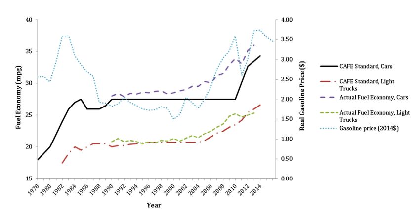
Additionally, other countries have been adopting increasingly strict standards for passenger vehicles and
light-duty trucks. Figure 2 shows that other countries have adopted higher standards that are applicable
today and reach the current U.S. targets earlier than would be required by the standards adopted for
upcoming model years. 14 And actual vehicle performance, in terms of fuel economy, already exceeds
the U.S.’s in the European Union, Japan, India, and China.
The upcoming NHTSA/EPA reassessment of the vehicle standards for MYs 2022-2025 will likely include a
benefit/cost analysis for any changes in those standards. One important assumption that underpins any
benefit/cost analysis of vehicle standards is the estimated size of the rebound effect, or how consumers
respond in VMT to increased (or decreased) cost of driving as a result of changes in fuel economy (e.g.,
how they might respond to reduced fuel economy in the event that the standards were weakened
relative to those previously adopted by the agencies).
In this paper, we review the literature on changes in consumers’ driving habits in response to changes in
the cost of driving (which many studies use as a proxy for changes in vehicle fuel economy) and the
dollar value of savings in expenditures on fuel. 15 We analyze the studies’ estimates of the rebound
effect and the impact on energy savings that result from changes in fuel prices or the cost of driving
Gasoline price ($/gallon) 2022 2023 2024 2025 2026 2027 2028 2029 2030
AEO 2015 Reference case (2013$) 2.82 2.86 2.90 2.95 3.00 3.04 3.09 3.14 3.20
AEO 2015 Reference case (2017$) 3.02 3.06 3.11 3.16 3.21 3.26 3.31 3.37 3.43
AEO 2018 Reference case (2017$) 3.13 3.18 3.25 3.25 3.24 3.26 3.29 3.33 3.34
See also Bordoff et al (2018), Figure 5.
12
Bordoff et al. (2018), page 10.
13
Bordoff et al. (2018), Figure 7, and pages 11-12. Note that the estimates of future market shares of light-duty
vehicles were lower in the AEO prepared in 2012 as compared to AEO 2015, but the projection of such market
share has declined in the AEO 2018 relative to the AEO 2015 (i.e., the one relied upon in the 2015
EPA/NHTSA/CARB 2016 Draft TAR).
14
Plummer and Popovich (2018).
15
One study (Linn (2013) explicitly attempts to estimate the rebound effect associated with changes in fuel
economy as opposed to changes in gasoline prices, but the relevance of Linn’s analysis for setting national fuel-
economy standards is complicated and lessened by the fact that he uses household survey data for only one year
(i.e., 2009) in which there were multiple and complex changes occurring in the economy (as discussed further
below), as well as techniques that attempt to account for any correlations that might exist between fuel economy
and other vehicle characteristics and for indirect effects on VMT associated with households’ ownership of more
than one vehicle.
Analysis Group 7Vehicle Fuel-Economy and Air-Pollution Standards: The Rebound Effect
(taking into account the dollar savings that results from vehicles’ ability to travel farther per gallon of
fuel).
Figure 2:
Comparing U.S. Fuel Economy Standards for Passenger Cars with the Rest of the World’s
(2000 to 2025)
Source: New York Times based on information from the International Council on Clean Transportation (Plummer
and Popovich (2018))
II. The “Rebound Effect”
Where the cost of energy is relevant to decisions about how much to use a product that consumes
energy, economic theory and empirical research suggests that when consumers switch from a less-
energy-efficient product (e.g., a standard sport utility vehicle (“SUV”)) to a more energy-efficient
product (e.g., an electric-hybrid SUV) that serves the same purpose, those consumers will increase their
use of the product: that is, greater fuel-economy leads to driving more miles. This is a phenomenon
known as the “rebound effect.” NHTSA and EPA define the rebound effect generally as "…the additional
energy consumption that may arise from the introduction of a more efficient, lower cost energy service
which offsets, to some degree, the energy savings benefits of that efficiency improvement.” 16
As an example of this rebound concept, consider a consumer who drives 100 miles each week in a car
achieving 20 MPG. She consumes 5 gallons of gasoline and, at $2/gallon of gasoline, she spends $10 a
week on fuel (equivalent to 10 cents per mile driven). If she were to buy a car with a rating of 25 MPG
(i.e., a 25-percent improvement in fuel economy) and assuming that gas prices remained fixed, she
would save 1 gallon of fuel (or $2 dollars for her overall gasoline expenses) per week; this equates to 8
16
EPA/NHTSA/CARB 2016 Draft TAR, Chapter 10.4, page 10-9.
Analysis Group 8Vehicle Fuel-Economy and Air-Pollution Standards: The Rebound Effect
cents per mile, or a 20-percent reduction in the out-of-pocket cost of driving. If the assessment stopped
there, however, it would ignore the rebound effect, because it would implicitly assume that the
consumer would continue to travel 100 miles per week, and her more fuel-efficient car would save her
20-percent in out-of-pocket gasoline costs. The higher fuel economy would make traveling a fixed
distance cheaper and the consumer would therefore tend to consume more of the good or service (e.g.,
driving) as it becomes less expensive. This suggests that one might expect this consumer to drive more
than 100 weekly miles with her more fuel-efficient car. The extent to which she exceeds 100 weekly
miles − if she does − is what we would call the magnitude of the “rebound effect.” 17 The magnitude of
the rebound effect may be affected by factors such as whether the amount of driving was influenced by
the cost of fuel, whether there is an unmet desire to drive more, and whether the additional driving is
not offset by other costs (such as time spent driving) that result from driving more miles.
Therefore, to make policy concerning the effectiveness of vehicle standards − to save gasoline and to
avoid GHG emissions − and to determine whether a new standard’s benefits exceed its costs, policy
makers need to make decisions taking into account reasonable estimates of the rebound effect. Doing
so will assist them in developing better-informed assessments of the impact of various proposed vehicle
standards on energy savings and avoided GHG emissions. The larger the rebound effect, the lower will
be the fuel savings and GHG emission reductions associated with a new, stricter vehicle standard (or the
lower will be the increases in fuel use and GHG emissions associated with a relaxation of the stringency
17
Different assumptions about the level of the rebound effect lead to different estimates of the gasoline cost
savings that would result from the more fuel-efficient vehicle. For example and building off of the hypothetical
case described above: The 25-percent improvement in fuel economy (switching from a car with 20 MPG to one
with 25 MPG) would allow the consumer to avoid purchasing one gallon of gasoline ($2) a week to drive her 100
miles per week. The cost of driving would go down from 10 cents per mile to 8 cents per mile. Her out-of-pocket
costs to purchase gasoline to drive 100 miles would decrease by 20 percent.
Using the EPA/NHTSA method to calculate the effect of rebound on changes in VMT (which is calculated as
the percentage difference in VMT = (rebound effect * (baseline fuel cost per mile - policy fuel cost per
mile)/baseline fuel cost per mile)), here are examples of the the impact:
If there were no rebound effect (i.e., a rebound effect of 0 percent), then she would have a gasoline cost
savings of 20 percent (or 2 cents per mile).
If there were a 10-percent rebound effect, she would increase her driving by 2 miles per week, for a total of
102 miles. (This is calculated as a 20-percent (0.2) reduction in the cost of driving times 10-percent (0.10)
rebound effect times 100 miles = 2 additional miles.) She would need to buy 4.08 gallons a week to drive 102
miles (i.e., (100+2) ÷ 25 MPG = 4.08 gallons per week). At $2/gallon, this would mean that she would spend
$8.16 per week on gasoline, which equates to an 18.4-percent reduction in fuel costs (i.e., from $10 to $8.16
per week).
If there were a 89-percent rebound effect, she would increase her driving by 17.8 miles per week, for a total of
117.8 miles. (This is calculated as a 20-percent (0.2) reduction in the cost of driving times the 89-percent
(0.89) rebound effect times 100 miles = 17.8 additional miles.) She would need to buy a total of 4.7 gallons
per week to drive 117.8 miles (i.e., (100+17.8) ÷ 25 MPG = 4.7 gallons of gasoline per week). At $2 per gallon,
she would spend $9.42 dollars per week on gasoline. Her car with a 25-percent increase in fuel economy
would save her 58 cents (or 5.8 percent) a week in gasoline costs.
The agencies’ method for calculating the rebound effect on VMT is found in their “Joint Technical Support
Document: Final Rulemaking for 2017-2025 Light-Duty Vehicle Greenhouse Gas Emission Standards and Corporate
Average Fuel Economy Standards,” August 2012. (U.S. EPA and NHTSA (2012), pages 4-15 and 4-16.)
Analysis Group 9Vehicle Fuel-Economy and Air-Pollution Standards: The Rebound Effect
of an existing vehicle standard). Thus, the benefits of adopting a change in a vehicle standard depends,
in part, on the magnitude of the rebound effect.
When EPA and NHTSA established the MY 2022-2025 standards, their review of the literature led them
to rely upon a 10-percent rebound effect as part of their calculation of benefits and costs of the new,
more stringent vehicle standards. 18 In an April 2018 notice signed by Administrator Pruitt regarding the
withdrawal of the EPA’s January 12, 2017 Final Determination on fuel economy standards for MYs 2022-
2025, EPA stated its intention to review the Obama Administration’s vehicle standard and to reconsider,
among other things, the record on how a rebound effect might affect an assessment of fuel and GHG
savings from the the standards. 19
In this paper, we review studies estimating the rebound effect and offer our own assessment regarding
the status of the literature and the implications for the appropriate choice of rebound effect for the
purposes of setting national vehicle standards for fuel economy and GHG emissions.
III. Review of the Rebound-Effect Literature Related to Fuel-
Economy Standards in Vehicles
We reviewed 35 journal articles and other analyses that either assessed and/or estimated the rebound
effect (as defined most typically in terms of changes in VMT as a result of a change in the price of
gasoline or in the cost of driving).
We drew our initial list of analyses from relevant sources cited by the EPA/NHTSA/CARB in their 2016
assessment of the CAFE and GHG standards, and further expanded our review based on literature cited
from two industry studies. 20 Appendix Table 2 lists the analyses and other documents we reviewed in
our evaluation and in preparing this report. Appendix Table 2 also summarizes the studies’ findings with
respect to the rebound effect.
Most of these original research studies have been described in some detail in other documents that
include literature reviews, such as the EPA/NHTSA/CARB 2016 Draft TAR, 21 and most recently by
researchers at the Department of Energy’s Lawrence Berkeley National Laboratory (“LBNL”). 22
Additionally, many of the journal publications and research reports include the author’s summary of
his/her own review of the rebound literature.
18
EPA/NHTSA/CARB 2016 Draft TAR, Chapter 10.4 generally, and specifically page 10-10.
19
U.S. EPA, “Notice of Revised Final Determination, Mid-term Evaluation of Greenhouse Gas Emissions Standards
for Model Year 2022-2025 Light-duty Vehicles,” Signed April 2, 2018, pages 2-3, 28.
https://www.eenews.net/assets/2018/04/03/document_cw_01.pdf.
20
These two industry-sponsored documents/studies were: Carlson et al. (2017); and McAlinden et al. (2016).
21
EPA/NHTSA/CARB 2016 Draft TAR, Section 10.4 (“Fuel Economy Rebound Effect”).
22
Wenzel and Fujita (2018), pages 1-8.
Analysis Group 10Vehicle Fuel-Economy and Air-Pollution Standards: The Rebound Effect
All the analyses we reviewed determined and/or commented on the rebound effect by estimating the
changes in consumers’ VMT in response to changes in the relative cost of fuel. 23 In effect, this depiction
of the rebound effect amounts to an estimation of the elasticity of demand for travel -- i.e., the
percentage change in one outcome (VMT) due to a unit percentage change in another (the cost of
driving a vehicle). 24
In addition, the contexts, methods and data used in the studies vary substantially. This leads to a
literature that produces a wide array of estimates of the rebound effect, with estimates ranging from a
low rebound effect of 0 percent (i.e., an increase of 0 percent in VMT) to a high rebound effect of 89
percent. There are multiple sources of these variations.
First, the studies rely on different types of data, with each data series providing a different lens for
viewing and understanding the topic. In general, the most recent data are for the year 2010 (as shown
in Appendix Table 2).
Some of the studies examine time-series data covering many decades (e.g, Greene (2012), examining
data from 1966-2007; Gately (1992), assessing data from 1966-1988; and Schimek (1996), relying on
data from 1950-1994).
Some studies examine behavior based on what happened during a single year (e.g., Linn (2013), Su
(2012) and Liu et al. (2014), each of which similarly analyzes the 2009 National Household Travel Survey
(“NHTS”) data). 25
Other studies examine data related to:
a particular geographic segment of the U.S. population (e.g., Gillingham et al. (2015), relying
upon vehicle odometer data collected in Pennsylvania’s emission inspection program for light-
23
Note the prior exception is Linn (2013), in which he analyses the effects of changes in fuel prices and changes in
fuel economy on VMT.
24
As discussed further below, this relationship between the fuel cost associated with driving and demand for travel
is not exactly the same as the change in VMT associated with changes in fuel economy per se, especially in light of
the fact that the latter may involve impacts related to differences in the purchase price of vehicles as well as
differences in operating costs of the vehicles, whereas changes in the cost of gasoline would likely only show up in
terms of the operating costs of vehicles over time.
25
“The 2009 NHTS is a nationally representative survey of travel behavior conducted from April 2008 through April
2009. This latest in the series updates information gathered in the Nationwide Personal Transportation Survey
(NPTS) conducted in 1969, 1977, 1983, 1990, and 1995, and the National Household Travel Survey conducted in
2001. The 2009 NHTS sample design was composed of two major sample units. The first sample unit contained
25,000 households representing all 50 U.S. States and the District of Columbia. The second unit was the Add-On
sample, which consisted of 20 states and Metropolitan Planning Organizations (MPOs) who collectively purchased
an additional 125,000 household samples for their respective regions. These two sample units brought the 2009
NHTS sample size to about 150,000 households and 300,000 people.” National Highway Administration,
Department of Transportatin, Summary of Travel Trends: 2009 National Household Travel Survey,” June 2011,
Section 1.0. https://nhts.ornl.gov/2009/pub/stt.pdf.
Analysis Group 11Vehicle Fuel-Economy and Air-Pollution Standards: The Rebound Effect
duty vehicles between 2000-2010; Gillingham (2014), analyzing data from California; Wenzel
and Fujita (2018), examining data from Texas), or
driving behavior in geographies outside of the U.S. (e.g., Chitnis et al. (2014), examining 2009
data from the United Kingdom; Frondel and Vance (2013), assessing data from Germany
between 1997-2009). 26
Second, the literature’s estimates of the rebound effect tend to vary according to whether researchers
assess the rebound effect over a short or longer time frame. In the short run, research suggests that
consumers may be less able to change behavior in response to changes in price, while they may have
more options over a longer period of time. 27 (For example, in the short run, they can drive less or take
advantage of travel options that already exist; over a longer period of time, they can purchase different
types of vehicles, in addition to the short-run options.) The fact that the rebound effect captures the
responsiveness of consumers to changes in relative travel costs suggests short-run rebound effects may
fall below long-run rebound effects. Small and Van Dender (2007a) indeed found a short-run rebound
effect of less than 5 percent, but a long-run rebound effect of over four times that amount. 28 According
to Linn (2013), “estimating long-run rebound introduces the typical challenges of estimating long run
responses while controlling for other factors that affect VMT such as income.” 29
Third, many researchers have uncovered other sources of differences in estimates of the rebound effect.
For example, several studies have found that the rebound effect appears to vary over time possibly due
to changing incomes and/or declining fuel prices. 30 Small and Van Dender (2007a) estimated a 22-
percent long-run rebound effect when analyzing the 1966-2001 time period; but when they limited the
analysis to the 1997-2001 period (a time during which consumers on average enjoyed higher incomes), 31
the authors found an 11-percent rebound effect and projected an even lower rebound effect in the
26
This variation appears to reflect differences in the rebound effect in U.S. versus other countries. For example,
Frondel and Vance (2013) used panel data collected in Germany for 1997-2009, and found a rebound effect of 46-
70 percent. Studying behaviors in the U.K., Chitnis et al. (2014) similarly estimated a rebound effect as high as 65
percent. In contrast, estimates sourced from U.S. data generally do not exceed 40 percent. See Appendix Table 2.
27
As described by researchers at the LBNL: “Actions households can take in response to changes in fuel price in
the short-run include changing driving patterns, or reallocating the total VMT of a household among the different
vehicles already owned by the household. Long-run responses to changes in fuel price include purchasing a
replacement vehicle, or changing home or work location.” Wenzel and Fujita (2018), page 2.
28
See Small and Van Dender (2007a); Hymel and Small (2015) find a similar relationship between short-run and
long-run rebound effects.
29
Linn (2013), page 2.
30
See Small and Van Dender (2007a); Hymel et al. (2010); Greene (2012).
31
See https://fred.stlouisfed.org/series/MEHOINUSA672N. In addition to income, other factors including the state
of the economy and fuel prices during the period studied can impact the rebound effect. As Liu et al. (2014) note:
“Changes in fuel cost have great effects on increasing/reducing vehicle usage, for example, vehicle usage will be
reduced by around 20% when the driving cost increases by 50%... It should be noted the dataset we used was
collected in 2009 when fuel prices were particularly high and that the conditions of the US economy at the time
were not particularly good.”
Analysis Group 12Vehicle Fuel-Economy and Air-Pollution Standards: The Rebound Effect
future. 32 Additionally, they have not attempted to take into consideration how the effect might change
in the fugure.
By contrast and based on his findings that rising incomes reduce the rebound effect, Greene (2012)
projected that the rebound effect could decrease by as much as 3.4 percentage points over the
subsequent two decades as per-capita income grows year-over-year (with rebound starting at 12
percent in 2008 and declining to 8.6 percent by 2030). 33
These studies suggest that with rising incomes and in periods of relatively low oil prices, the rebound
effect will be smaller over time. Hymel et al. (2010) found that rising income and increased congestion
contribute to a lower rebound effect (because “people with higher incomes have a higher value of time
and are more easily dissuaded from driving when faced with congestion costs” 34). 35 Su (2012) also
found that congestion, among other things, affects the size of the rebound effect by dampening the
demand for travel: “The sensitivity of travelers’ demand in terms of VMT to the fuel cost per mile and
other important determinants such as road density, population density, congestion, and public transit
supply, therefore, could be different given this wide gap of VMT.” 36
Fourth, many studies estimating the rebound effect do so by determining the impact of changes in fuel
prices on VMT. The application of such studies to the fuel economy context explicitly or implicitly
assumes that consumers do not distinguish between a change in fuel price and a change in fuel
economy: this assumption, for example, reflects the point of view that a decrease in fuel prices and an
increase in fuel economy both decrease the relative out-of-pocket cost of driving for consumers.
Three recent analyses demonstrate, however, that such an assumption may not be appropriate: Greene
(2012) found that consumers respond to fuel price, but not fuel economy (implying a zero-percent
rebound effect for increases in fuel economy). He posits that consumers may respond differently to
32
Small and Van Dender found that “the VMT and rebound effects are affected by per capita income, fuel costs,
and urbanization….The strongest influence is income, the second strongest is fuel costs. Because incomes rose but
fuel costs per mile fell over this period, both sources of variation caused the rebound effect to decline. This decline
is substantial: we calculate that over the last five years of the sample, the rebound effect was only about one-
fourth as large as its average over the entire period. This means that fuel economy improvements are more
effective at reducing fuel consumption now than they were in the past….Because we isolate the factors causing
this decline [in the rebound effect], we can also say something about future trends. Projections by the Energy
Information Agency show per capita income continuing its steady rise, while gasoline prices are expected to be flat
or possibly to rise slowly. (Both income and fuel price are here expressed in constant dollars.) Furthermore, the
elasticities we measure are about four times more sensitive to income than to fuel costs; and even if gasoline
prices rise further, fuel costs per mile probably won’t, because of improvements in fuel efficiency. Therefore, it
seems to us extremely likely that the price elasticity of gasoline will continue to fall slowly, and that the rebound
effect will decline to a very small value.” Small and Van Dender (2007b), page 13.
33
See Greene (2012), Table A1. This projection assumed that real per-capita income would rise 1.5 percent per
year over this period.
34
Hymel et al. (2010), page 20.
35
Note that the EIA 2018 Annual Energy Outlook projects that that real personal income per capita in the U.S. is
expected to grow 40 percent from 2017 to 2037.
36
Su (2012), page 369.
Analysis Group 13Vehicle Fuel-Economy and Air-Pollution Standards: The Rebound Effect
these two factors that affect the cost of driving: on the one hand, he discusses how improved fuel
economy changes the cost of driving through vehicle manufacturers’ installation of fuel-efficient
equipment that raises the initial cost of the vehicle to the consumer (but not necessarily in a visible
way); on the other, changes in the price of gasoline occur more transparently and influence how a driver
understands changes in the variable cost of operating the vehicle. Greene states that “[u]sing national
time series data for 1966 to 2007, this study finds a statistically significant elasticity of vehicle travel with
respect to fuel price, but no statistically significant elasticity of vehicle travel with respect to fuel
economy. … What is new is the finding that the hypothesis that the elasticities of vehicle travel with
respect to fuel price and fuel economy (gallons per mile) are equal, as predicted by theory, is now
rejected by the national time series data.” 37
In his analysis of household survey data for the year 2009, Linn (2013) found that consumers respond
less to changes in fuel price than to changes in fuel economy. Linn posits that because consumers may
perceive the latter to be more persistent (i.e., affecting the basic MPG of a vehicle) than the former
(e.g., reflecting fluctuations in the price of gasoline over time), consumers change their travel behavior
more in response to the effect of fuel economy on the cost of driving. 38
In their study of driving patterns in Texas, Lawrence Berkeley National Laboratory’s Wenzel and Fujita
(2018) measured the change in VMT in response to a change in the price of gasoline as well as in relation
to the “cost of driving”, with the latter using “rated combined city/highway fuel economy of each vehicle
to calculate the cost of driving, in cents per mile, since the vehicle’s previous inspection (price of
gasoline divided by the vehicle’s fuel economy)….. [They] found that a one percent increase in the cost
of driving is associated with a decrease in VMT (0.16% decrease) nearly twice as large as a one percent
increase in the price of gasoline (0.09% decrease in VMT), after accounting for vehicle make and
model.” 39 This finding suggests that they agree with Linn that consumers respond less to changes in fuel
price than to changes in fuel economy. Also, Wnezel and Fujita (2018) conclude that “[f]or most vehicle
types, vehicles with relatively low fuel economy have a larger decrease in VMT in response to an
increase in the price of gasoline than vehicles with relatively high fuel economy;... By effectively
decreasing the price of gasoline, fuel economy standards are likely to induce drivers of new, relatively
high MPG vehicles to increase their VMT. Our analysis by rated fuel economy suggests that increased
fuel economy standards will induce drivers of high MPG vehicles to increase their VMT, by 15% in CUVs
[cross-over utility vehicles], 10% in small pickups and SUVs, 7% in minivans, and less than 1% in cars. We
estimate the weighted average VMT increase in new high MPG vehicles to be 5.2%.” 40
37
Greene (2012), page 26.
38
Linn (2013), pages 9, 15-16.
39
Wenzel and Fujita (2018), page iv. Also, they report that “[a]dding variables to account for the median
household income or population density of the zip code in which the vehicle is registered, or including an
instrument to address potential endogeneity in gas prices, slightly reduces this estimate. [Their] result suggests
that the rebound effect in Texas is slightly lower than that in California and Pennsylvania using similar vehicle-level
data.” Page iii.
40
Wenzel and Fujita (2018), page 45.
Analysis Group 14Vehicle Fuel-Economy and Air-Pollution Standards: The Rebound Effect
Fifth, the rebound effect has been found to be smaller in situations where gasoline price cuts occurred
(i.e., where the cost of driving went down) as compared to when price increases were taking place.
Gately (1992) found that during the 1966-1988 period, the rebound effect associated with changes in oil
price is asymmetrical and “data show smaller response to price cuts than to price increases.” The
Hymel and Small (2015) estimated an 18-percent long-run rebound effect when assessing the 2000-2009
time period, and that “the rebound effect is much greater in magnitude in years when gasoline prices
are rising than when they are falling. It is also greater during times of media attention and price
volatility, which explains about half the upward shift just mentioned.
Wenzel and Fujita (2018) observed that “[s]ince light-duty vehicle standards would be expected to lower
the cost of driving, this would suggest that the lower estimate of the price elasticity of VMT would likely
be the appropriate elasticity to use when analyzing the impacts of light-duty vehicle standards….Hymel
and Small (2015) find that response to price rise is quick (i.e., largest in year of and year following the
change) and adjustment following a price drop occurs more slowly (i.e., small in year of and larger in
year following the change). This suggests that there is some ‘stickiness’ in consumer behavior that could
potentially mitigate rebound following a fuel-economy-driven decrease in the cost of driving.” 41
Finally, two recent industry-sponsored reports estimate the value of the rebound effect based on
reviewing the literature. 42 As part of a memorandum addressing EPA’s January 2017 Final
Determination of the Mid-Term Evaluation of Greenhouse Gas Emissions Standards for Model Years
2022-2025 Light-Duty Vehicles, Carlson et al. (2017) calculated the mean and median of a series of long-
run rebound effect estimates derived from several articles (which we reviewed). 43 In effect, Carlson et
al. assign equal weight to the long-run rebound estimates produced in the many studies, averaged them
to produce a rebound estimate, and concluded that a 20-percent rebound effect represents the
observations in the literature. McAlinden et al. (2016) 44 also suggested that a 20-percent rebound effect
was appropriate to use in their analysis of the net benefits of fuel economy standards set for 2017-2025.
They base this determination on five papers (all of which we also reviewed for this analysis), 45 but
provide little information that would explain the basis for their choice of a 20-percent rebound effect.
41
Wenzel and Fujita (2018), page 3, where they describe Hymel and Small (2015).
42
The automotive industry sponsored both reports (Carlson et al. (2017) and McAlinden et al. (2016))
43
In particular, these papers were listed in Carlson et al.’s Table 4 (Estimates of Long-run Rebound Effects Cited by
EPA). See Carlson et al. (2017). We note that we have also reviewed many of these papers and include them in
Appendix Table 2.
44
See McAlinden, et al., “The Potential Effects of the 2017-2025 EPA/NHTSA GHG/Fuel Economy Mandates on the
U.S. Economy, Center for Automotive Research, September 2016.
45
See Greene et al. (1999); Small and Van Dender (2007a); Hymel et al. (2010); Linn (2013); and Greene (2012).
Analysis Group 15Vehicle Fuel-Economy and Air-Pollution Standards: The Rebound Effect
IV. Observations and Conclusions
The original research on the rebound effect conducted in the past two decades by scholars at
universities, national laboratories and other institutions has resulted in a growing literature of technical
studies that analyze numerous data sources.
The wide range of estimates of the rebound effect that this body of research produces makes it
important to identify which ones are appropriate and relevant for policy to ensure rigorous estimates of
the benefits and costs of a particular proposed fuel economy standard. As described above in the prior
section and as shown in Appendix Table 2, the estimates range from a low rebound effect of 0 percent
(i.e., no rebound effect at all) to a high rebound effect of 89 percent.
This wide range of estimates was explicitly acknowledged in the EPA/NHTSA/CARB 2016 Draft TAR,
when the agencies determined that a 10-percent rebound effect was appropriate to rely upon in setting
the fuel-economy and GHG standards for upcoming vehicle MYs. 46
As discussed above, there are many factors that help to explain the variation in estimates of the
rebound effect. The body of studies examine different questions (including how to measure and
estimate the rebound effect, and what methods to use to do so). They analyze different types of data,
which vary by: time (e.g., many years of data, versus a single year of data); place (e.g., national US data
versus data for particular parts of individual states versus data in other countries); variables of interest
(e.g., odometer data from vehicles; survey data from households; aggregate data on VMT; monthly data
on gasoline prices); and period over which the rebound effect is examined (e.g., short-run versus long-
run). Many of the studies looked at data during years when there was variation in the price of gasoline,
on the one hand, but long periods in which fuel economy remained relatively constant, on the other
(See Figure 1).
Thus, the contexts, methods and data used in the studies vary substantially, leading to a literature that
produces a wide array of estimates of the rebound effect.
Moreover, the literature suggests that, even if there were complete agreement about what the rebound
effect has been in the past, this would not necessarily provide reliable estimates of what such an effect
would be in the future -- especially in light of changing vehicle technologies, changing consumer
46
EPA/NHTSA/CARB 2016 Draft TAR, Section 10.4.4 (“Basis for Rebound Effect Used in the Draft TAR”). For
example, “there is a wide range of estimates for both the historical magnitude of the rebound effect and its
projected future value, and there is some evidence that the magnitude of the rebound effect appears to be
declining over time for those studies that look at VMT time trends. The recent literature is mixed, with some
studies supporting relatively modest direct VMT rebound estimates and other studies suggesting a higher rebound
effect. Some of these studies come to these varied conclusions despite using the same dataset. EPA and NHTSA
use a single point estimate for the direct VMT rebound effect as an input to the agencies' analyses, although a
range of estimates can be used to test the sensitivity to uncertainty about its exact magnitude. Based on a
combination of historical estimates of the rebound effect and more recent analyses, an estimate of 10 percent for
the rebound effect is used for evaluating the MY2022–2025 standards in this Draft TAR (i.e., we assume a 10
percent decrease in fuel cost per mile from the standards would result in a 1 percent increase in VMT).”
Analysis Group 16You can also read