Forward and Spot Exchange Rates in a Multi-Currency World
←
→
Page content transcription
If your browser does not render page correctly, please read the page content below
Forward and Spot Exchange Rates
                       in a Multi-Currency World∗
                       Tarek A. Hassan†                     Rui C. Mano‡

                                 Preliminary and Incomplete

                                              Abstract

          We decompose the covariance of currency returns with forward premia into a cross-
      currency, a between-time-and-currency, and a cross-time component. The surprising
      result of our decomposition is that the cross-currency and cross-time-components account
      for almost all systematic variation in expected currency returns, while the between-time-
      and-currency component is statistically and economically insignificant. This finding has
      three surprising implications for models of currency risk premia. First, it shows that
      the two most famous anomalies in international currency markets, the carry trade and
      the Forward Premium Puzzle (FPP), are separate phenomena that may require separate
      explanations. The carry trade is driven by persistent differences in currency risk premia
      across countries, while the FPP appears to be driven primarily by time-series variation in
      all currency risk premia against the US dollar. Second, it shows that both the carry trade
      and the FPP are puzzles about asymmetries in the risk characteristics of countries. The
      carry trade results from persistent differences in the risk characteristics of individual
      countries; the FPP is best explained by time variation in the average return of all
      currencies against the US dollar. As a result, existing models in which two symmetric
      countries interact in financial markets cannot explain either of the two anomalies.

JEL Classification: F31, G12, E36
Keywords: Risk Premia in Foreign Exchange Markets, Forward Premium Puzzle, Carry
Trade
   ∗
     We are grateful to Craig Burnside, John Cochrane, Jeremy Graveline, Ralph Koijen, Matteo Maggiori,
and Adrien Verdelhan. We also thank seminar participants at the University of Chicago, CITE Chicago, the
Chicago Junior Finance Conference, KU Leuven, University of Sydney, New York Federal Reserve, University
of Zurich, SED annual meetings , and the NBER Summer Institute for useful comments. All mistakes remain
our own.
   †
     University of Chicago, Booth School of Business, NBER and CEPR, 5807 South Woodlawn Avenue,
Chicago IL 60630 USA; E-mail: Tarek.Hassan@ChicagoBooth.edu.
   ‡
     International Monetary Fund, Research Department

                                                   1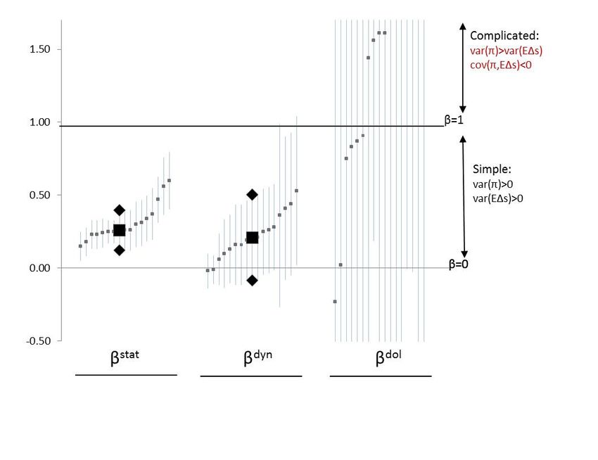
1       Introduction
The forward premium puzzle and the carry trade anomaly are two major stylized facts in
international economics. In this paper we introduce a decomposition that allows us to show
analytically how the two anomalies relate to each other and to estimate the joint restrictions
they place on models of currency risk premia and exchange rate determination.
    The forward premium puzzle is usually documented using a bilateral regression of currency
returns on forward premia:

                                   rxi,t+1 = αi + β fi pp (fit − sit ) + εi,t+1 ,                              (1)

where fit is the log one-period forward rate of currency i , sit is the log spot rate and rxi,t+1 =
fit − si,t+1 is the log excess return on currency i between time t and t + 1.1 Although estimates
of β fi pp tend to be noisy, we tend to find β fi pp > 0 for most currencies. A pooled specification
that constrains all β fi pp to be identical across currencies yields point estimates significantly
larger than zero and often larger than one. This fact, the forward premium puzzle (FPP),
has drawn a lot of interest by theorists because it has apparently complex implications for the
joint dynamics of currency risk premia, interest rates, and exchange rates. For example, Fama
(1984) shows that β fi pp > 1 implies that bilateral currency risk premia must be highly volatile
and negatively correlated with expected depreciations.2 This fact is usually interpreted to
mean that (i) the carry trade, a trading strategy which is long high interest rate currencies
and short low interest rate currencies, is profitable due to the FPP; (ii) bilateral currency
risk premia are highly elastic with respect to time series variation in forward premia; and (iii)
these elasticities tend to be larger than one, such that they must play a role in determining
bilateral exchange rates.
    In this paper we generalize the regression-based approach in (1) to study the covariance
of currency risk premia with forward premia without conditioning on a specific currency pair
i. We decompose the unconditional covariance into a cross-currency, a between-time-and-
currency, and a cross-time component. Each of the three components can be written either
as the expected return to a trading strategy or as a function of a slope coefficient from a
regression that relates variation in currency returns to variation in forward premia in the
corresponding dimension.
    1
     The same relationship is often estimated using the change in the spot exchange rate as the dependent
variable, in which case the coefficient estimate is 1 − β fi pp . An equivalent way of stating the FPP is thus that
1 − β fi pp < 0.
   2
     Throughout the paper we follow the convention in the literature and refer to conditional expected returns
as “risk premia”. However, this terminology need not be taken literally. Our analysis is silent on whether
currency returns are driven by risk premia, institutional frictions, or other limits to arbitrage. See Burnside
et al. (2011) and Lustig et al. (2011) for a discussion.

                                                         2
Our decomposition shows that the expected return on the carry trade is the sum of the
cross-currency and the between-time-and currency component of the unconditional covariance,
while the forward premium puzzle consists of the sum of the between-time-and currency and
the cross-time components.
By estimating the elasticity of risk premia with respect to forward premia in each of these
dimensions, we show that most of the systematic variation in currency returns is in the cross-
section (the cross-currency variation in αi in (1)). Currencies that have persistently higher
forward premia pay significantly higher expected returns than currencies with persistently
lower forward premia. Some of our specifications also show statistically significant variation
in the cross-time dimension: expected returns on the US dollar appear to fluctuate with its
average forward premium against all other currencies in the sample. This cross-time variation
is particular to the US dollar and, potentially, a small number of other currencies. It explains
the vast majority of the variation that generates the forward premium puzzle. In contrast, we
cannot reject the null that currency risk premia do not fluctuate between-time-and-currency.
Once the average forward premium of all currencies against the US dollar is controlled for,
there is little evidence of additional covariance between risk-premia and forward premia in the
time series dimension.
Moreover, none of the three elasticities we estimate is significantly larger than one such
that we cannot reject the hypothesis that risk premia and expected changes in exchange rates
are uncorrelated in the data.
These results imply that the traditional interpretation of the FPP is misleading: the carry
trade and the FPP are not significantly related in the data and may thus require distinct
theoretical explanations. Explaining the carry trade primarily requires explaining persistent
differences in interest rates across currencies that are partially, but not fully, reversed by
predictable movements in exchange rates. (High interest rate currencies depreciate, but not
enough to reverse the higher returns resulting from the interest rate differential.) In contrast,
explaining the FPP may require explaining the time series variation in the risk premium of
the US dollar against all other currencies. The US dollar may be one of a small number of
currencies that pays higher expected returns when its interest rate is high relative to its own
currency-specific average and to the world average interest rate at the time. However, this
relationship is only marginally statistically significant in the data.
Part of the reason for our failure to find evidence of a covariance of risk-premia with forward
premia in the between-time-and-currency dimension is that the forward premium puzzle itself
greatly diminished once we stop conditioning on a specific currency pair i.
We show that, when using data for more than one currency, an unbiased estimate of the
elasticity of risk premia with respect to forward premia requires using out-of-sample regres-
3sions, such that the right hand side variables that predict returns between t and t + 1 are
known at time t. Since each of our regressions maps into a trading strategy, this result appears
only natural: when we estimate the expected returns on a given trading strategy we typically
require that all information used in the formation of the portfolio is available ex-ante. For
example, an investor who plans to go long a currency when its forward premium is higher
than its unconditional mean needs to estimate this unconditional mean using data available
at t. Similarly, when we estimate the elasticity of behavior (demanding a risk premium) with
respect to some right hand side variable, this variable needs to be measurable at time t.
In contrast, measures that do not correct for the fact that the sample mean of each cur-
rency’s forward premium is unknown ex-ante may not produce unbiased estimates of the true
elasticity of risk-premia with respect to forward premia. In particular, the pooled version of
(1) that constrains all β fi pp to be equal across currencies produces an upwardly biased measure
of the elasticity of risk-premia with respect to forward premia in the time-series dimension. In
other words, skimming across a table that lists β fi pp for each currency and mentally averaging
across these estimates is not innocuous and makes the forward premium puzzle appear more
severe than it actually is. For example, in our standard specification the weighted average
of β fi pp is 1.81 (s.e.=0.53), while our unbiased point estimate for the elasticity of risk-premia
with respect to forward premia in the time-series dimension is only half that number (0.86,
s.e.=0.34).
The summary of our results poses a challenge to the traditional interpretation of the
forward premium puzzle in the sense that currency risk premia may be much simpler objects
than previously thought. First, the majority of the variation in currency risk premia is static
(or highly persistent) across currencies. Second, we find no statistically reliable evidence
supporting the idea that currency risk premia respond to deviations of forward premia from
their time and currency specific mean. Third, we can never reject the hypothesis that the
elasticity of risk-premia with respect to forward premia in any of the three dimensions is
larger than one. As a result, we can never reject the hypothesis that currency risk premia are
uncorrelated with expected changes in exchange rates, neither for the US dollar nor for any
of the other currencies in our sample.
The bad news is that the persistent differences in interest rates driving the carry trade
are not well understood. Most existing models of currency risk premia focus on two ex-ante
symmetric countries and are thus calibrated to explain the relatively small and statistically
insignificant between-time-and-currency dimension of the covariance of risk premia with for-
ward premia.3 Many of these models may thus have to be re-interpreted in the light of our
evidence. The relatively small number of papers offering theoretical explanations of persis-
3
Examples include Farhi and Gabaix (2008), Verdelhan (2010), Burnside et al. (2009), Heyerdahl-Larsen
(2012), Yu (2011), Bacchetta et al. (2010), and, Ilut (2012).
4tent asymmetries in currency risk premia include Hassan (2013), Martin (2012), and Govillot,
Rey, and Gourinchas (2010) who focus on differences in country size, Maggiori (2013) and
Caballero, Farhi, and Gourinchas (2008) who focus on differences in financial development,
Ready, Roussanov, and Ward (2013) who focus on production specialization, and Mark and
Berg (2013) who focus on asymmetries in the conduct of monetary policy and degree of price
stickiness. Another strand of the literature has connected persistent currency risk premia
with shocks that are themselves persistent as in Engel and West (2005) and the long-run risk
model of Colacito and Croce (2011).
Our work builds heavily on a series of papers that apply factor analysis to study the cross
section of multilateral currency returns. Most closely related are Lustig, Roussanov, and
Verdelhan (2010, 2011) who identify a risk-factor that explains the cross section of currency
returns and a “dollar factor” that explains the time series variation in the returns on the US
dollar.4 Our contribution is to re-cast these findings in terms of regression coefficients, relate
them to established puzzles in the literature, and to translate them into restrictions on linear
models of currency risk premia.
Many authors have described and theorized about the carry trade and the FPP.5 We
contribute to this literature in three ways. First, we show that the carry trade and the
FPP are distinct, quantitatively unrelated, anomalies in the data. Second, we generalize the
empirical approach that has framed the debate on the FPP to a multi-currency framework.
Third, we use this framework to derive restrictions on linear models of multilateral currency
risk premia.
The remainder of this paper is structured as follows: Section 2 describes the data. Section
3 establishes the FPP and the carry trade as separate anomalies. Section 4 discusses the
restrictions that our empirical results pose on linear models of currency risk premia. Section
5 discusses implications for models of exchange rate determination. Section 6 concludes.
2 Data
Throughout the main text we use monthly observations of US dollar-based spot and forward
exchange rates at the one, six, and twelve month horizon. All rates are from Thomson Reuters
4
Also see Koijen et al. (2013) who decompose carry trades in different asset classes into static and dynamic
components.
5
See for example Hansen and Hodrick (1980), Bilson (1981), Meese and Rogoff (1983), Fama (1984), Backus
et al. (1993), Evans and Lewis (1995), Bekaert (1996), Bansal (1997), Bansal and Dahlquist (2000), Backus
et al. (2001), Evans and Lyons (2006), Graveline (2006), Burnside et al. (2006), Lustig and Verdelhan (2007),
Brunnermeier et al. (2009), Alvarez et al. (2008), Jurek (2009), Bansal and Shaliastovich (2010), Burnside
et al. (2011), Colacito and Croce (2011), Sarno et al. (2012), and Menkhoff et al. (2012). Engel (1996) and
Lewis (2011) provide excellent surveys.
5Financial Datastream. The data range from October 1983 to June 2010. For robustness checks
we also use all UK pound-based data from the same source as well as forward premia calculated
using covered interest parity from interbank interest rate data, which is available for longer
time horizons for some currencies. Our dataset nests the data used in recent studies on the
cross section of currency returns, including Lustig et al. (2011) and Burnside et al. (2011). In
additional robustness checks we replicate our findings using only the subset of data used in
these studies.
Many of the decompositions we perform require balanced samples. However, currencies
enter and exit the sample frequently, the most important example of which is the euro and
the currencies it replaced. We deal with this issue in two ways. In our baseline sample (“1
Rebalance”) we use the largest fully balanced sample we can construct from our data by
selecting the 15 currencies with the longest coverage (the currencies of Australia, Canada,
Denmark, Hong Kong, Japan, Kuwait, Malaysia, New Zealand, Norway, Saudi Arabia, Singa-
pore, South Africa, Sweden, Switzerland, and the UK from December 1990 to June 2010). In
addition, we construct three alternative samples which allow for entry of currencies at 3, 6,
and 12 dates during the sample period, where we chose the entry dates to maximize coverage.
The “3 Rebalance” sample allows entry in December of 1989, 1997, and 2004 and covers 30
currencies. The “6 Rebalance” sample allows entry in December of 1989, 1993, 1997, 2001,
2004, and 2007 and covers 36 currencies. Our largest sample, “12 Rebalance”, allows entry
in June 1986, and in June of every second year thereafter through June 2008 and covers 39
currencies. In between each of these dates all samples are balanced except for a small number
of observations removed by our data cleaning procedure (see appendix for details). Curren-
cies enter each of the samples if their forward and spot exchange rate data is available for at
least four years prior to the re-balancing date (the reason for this prior data requirement will
become apparent below).6
Throughout the main text we take the perspective of a US investor and calculate all returns
in US dollars. In Section 4.5 we discuss how our results change when we use different base
currencies.
Appendix A lists the coverage of individual currencies and describes our data selection
and cleaning process in detail.
6
The only exception we make to this rule is for the first set of currencies entering the 12 Rebalance sample
which become available in October 1983.
63 FPP & Carry Trade as Separate Anomalies
Consider a version of the carry trade in which, at the beginning of each month, t = 1, ...T ,
we form a portfolio of all available foreign currencies, i = 1, ..N , weighted by the difference
of their forward premia (f pit ≡ fit − sit ) to the average forward premium of all currencies
at the time (f pt ≡ i N1 f pit ). This portfolio is long currencies that have a higher forward
P
premium than the average of all currencies at time t and short currencies that have a lower
than average forward premium. We can write the expected return on this portfolio as
E [rxi,t+1 (f pit − f pt )] , (2)
where
T X N Z
X 1
E [·] ≡ (·) dFit (rxit+1 , f pit , f pjt , ...) (3)
t=1 i=1
N T
is the unconditional expectations operator defined over a finite number of currencies and time
periods, and Fit (rxit+1 , f pit , f pjt , ...) is some joint cumulative distribution function of the
returns on currency i at time t and the vector of forward premia of all currencies around the
world7 .
We use linear portfolio weights (f pit − f pt ), because they allow us to relate portfolio
returns directly to coefficients in linear regressions. Our results would be similar if we sorted
currencies into bins and then analyzed the returns on a long-short strategy as in Lustig et al.
(2011).8 As with this alternative formulation, the return on the carry trade portfolio is neutral
with respect to the dollar, i.e. it is independent of the bilateral exchange rate of the US dollar
against any other currencies.9
Table 1 shows the annualized mean return on the carry trade portfolio in our 1 Rebalance
sample. Consistent with earlier research, the carry trade is highly profitable and yields a mean
annualized net return of 4.95% with a Sharpe Ratio of 0.54. However, the table also shows
that currencies that the carry trade is long (i.e. currencies with high interest rates) on average
depreciate relative to currencies with low interest rates. Our carry trade portfolio loses 2.15
percentage points of annualized returns due to this depreciation. As we show below, this is a
general feature of the carry trade that holds across a wide range of plausible variations.
[Table 1 about here]
Currencies with high interest rates thus tend to depreciate. An obvious question is then
7
See Appendix B.1 for some properties of this expectations operator.
8
See Appendix Table 1 for a detailed comparison between linear weights (2), the long-short strategy of
Lustig et al. (2011), and the equally weighted strategy in Burnside et al. (2011).
9
See Appendix B.2 for a formal proof of this statement.
7why the FPP appears to suggest the opposite. The answer is in the currency-specific intercepts
in (1), αi . We tend to find that β fi pp > 1 in regressions in which currency fixed effects absorb
T
1
P
the currency-specific mean forward premium (f pi ≡ T
f pit ). If we wanted to trade on the
t=1
correlation in the data that drives the FPP, we would thus have to buy currencies that have
a higher forward premium than they usually do (Cochrane, 2001). Such a strategy, we call it
the “forward premium trade”, weights each currency with the deviation of its current forward
premium from its currency-specific average. We can write the expected return on the forward
premium trade as E [rxi,t+1 (f pit − f pi )] .
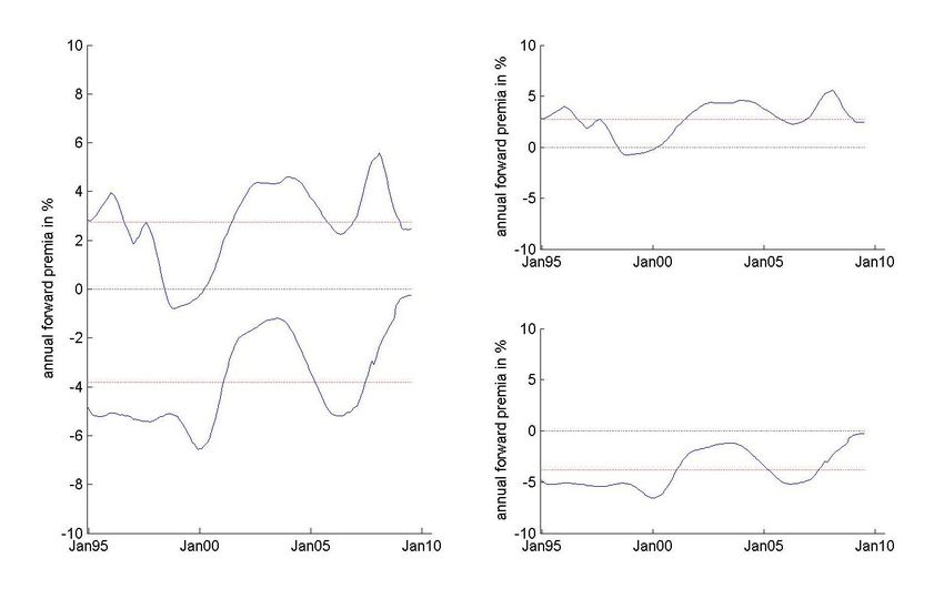
[Figure 1 about here.]
The carry trade (2) thus exploits a correlation between currency returns and forward
premia conditional on time, while the FPP describes a correlation conditional on currency.
Figure 1 illustrates the difference between the carry trade and the forward premium trade
for the case in which a US investor considers investing in two foreign currencies. The left
panel plots the forward premium of the New Zealand dollar and the Japanese yen over time.
Throughout the sample period the forward premium of the former is always higher than the
forward premium of the latter, reflecting the fact that New Zealand has consistently higher
interest rates than Japan. The carry trade is always long New Zealand dollars and always
short Japanese yen. In contrast, the forward premium trade evaluates the forward premium
of each currency in isolation and goes long if the forward premium is higher than its sample
mean. As a result, the forward premium trade is not “dollar neutral” in the sense that it may
be long or short both foreign currencies at any given point in time.
It is immediately apparent that the forward premium trade may be more difficult to
implement in practice than the carry trade as it requires an estimate of the mean forward
premium of each country (f pi ), which is not known at time t. In what follows we denote the
expectation of the country-specific and the unconditional mean forward premium as
fˆpi ≡ Ei [f pi ] , fˆp ≡ E [f p] ,
T
1
P R
where Ei [·] = T
(·) dFit (rxit+1 , f pit , f pjt , ...) and we continue the convention of denoting
t=1
sample means by omitting the corresponding subscripts,
1
PT 1
PN 1
PT PN
xi ≡ T t=1 xit xt ≡ N i=1 xit x ≡ NT t=1 i=1 xit , x = f p, rx . (4)
The ex-ante implementable version of the forward premium trade (which we show below is
the version that is relevant for estimating covariances of risk premia and forward premia) has
8average returns of h i
E rxi,t+1 f pit − fˆpi , (5)
where fˆpi 6= f pi and fˆp 6= f p in a finite sample (T < ∞).
How do the carry trade and the forward premium trade relate to each other? The expected
returns on both portfolios load on different components of the unconditional (population)
covariance between currency returns and forward premia. To see this we can decompose the
unconditional covariance into the sum of the expected returns on three trading strategies plus
a constant term. Re-writing the covariance in expectation form, adding and subtracting f pt ,
fˆpi , and fˆp and re-arranging yields
h cov h , f pit )= E [(rxi,t+1 −
i (rxi,t+1 − f p)] h
rx) (f piti i
ˆ ˆ ˆ
= E rxi,t+1 f pi − f p + E rxi,t+1 f pit − f pt − f pi − f p ˆ ˆ
+ E rxi,t+1 f pt − f p
| {z } | {z } | {z }
Static Trade Dynamic Trade Dollar Trade
+E [rxi,t+1 ( fˆp − f p )],
| {z }
Constant
(6)
where rx again refers to the sample mean currency return across currencies and time periods.
The “Static Trade” trades on the cross-currency variation in forward premia. It is long
currencies that have an unconditionally high forward premium and short currencies that have
an unconditionally low forward premium. We may think of it as a version of the carry trade
in which we never update our portfolio. We weight currencies once, based on our expectation
of the currencies’ future mean level of interest rates and never change the portfolio thereafter.
The “Dynamic Trade” trades on the between time and currency variation in forward premia.
It is long currencies that have high forward premia relative to the time average forward
premium of all currencies and relative to their currency-specific mean forward premium. We
may think of the expected return on the Dynamic Trade as the incremental benefit of re-
weighing the carry trade portfolio every period. Finally, the “Dollar Trade” trades on the
cross-time variation in the average forward premium of all currencies against the US dollar.
It goes long all foreign currencies when the average forward premium of all currencies against
the US dollar is high relative to its unconditional mean and goes short all foreign currencies
when it is low.10
Upon inspection, the carry trade (2) is simply the sum of the Static and Dynamic trades,
h i h i
E [rxi,t+1 (f pit − f pt )] = E rxi,t+1 fˆpi − fˆp + E rxi,t+1 f pit − f pt − fˆpi − fˆp
| {z } | {z } | {z }
Carry Trade
Static Trade Dynamic Trade
10
The Dollar Trade was first described by Lustig et al. (2010). We follow their naming convention here.
9while the forward premium trade (5) is the sum of the Dynamic and the Dollar Trades.
h i h i h i
ˆ ˆ ˆ
E rxi,t+1 f pit − f pi = E rxi,t+1 f pit − f pt − f pi − f p ˆ
+ E rxi,t+1 f pt − f p
| {z } | {z } | {z }
FP Trade Dynamic Trade Dollar Trade
The common element between the Carry Trade and the FPT is the Dynamic Trade, i.e. the
between-time-and-currency part of the unconditional covariance between currency returns and
forward premia. In contrast, the cross-currency component is unique to the carry trade and
the cross-time component is unique to the FPT. The question of whether the two anomalies,
the carry trade and the FPT, are related in the data thus reduces to estimating the relative
contribution of the Dynamic Trade.
[Table 2 about here]
Table 2 lists the mean returns and Sharpe ratios of the three strategies, as well as the mean
returns and Sharpe ratios of the carry trade and the forward premium trade. All returns are
again annualized and normalized by dividing with f p to facilitate comparison. Columns 1-4
on the top left give the results for our 1 Rebalance sample, where we use all available data
prior to December 1994 to estimate fˆpi and fˆp. Column 1 shows the results for one-month
forwards, without taking into account bid-ask spreads. The mean annualized return on the
static trade is 3.46% with a Sharpe ratio of .39. It thus contributes 70% of carry trade returns.
In contrast, the Dynamic Trade contributes 30%, with an annualized return of 1.50% and a
Sharpe ratio of .24.
Although the forward premium trade is not commonly known as a trading strategy in
foreign exchange markets it yields similar returns to the carry trade, with a mean annualized
return of 4.04% and a Sharpe ratio of .27. The Dollar Trade contributes 63% to this overall
return and has a Sharpe ratio of .25, with the Dynamic Trade contributing the remaining
37%.
Columns 2-4 replicate the same decomposition but take into account bid-ask spreads in
forward and spot exchange markets.11 Column 2 again uses one-month forward contracts,
column 3 uses 6-month contracts, and column 4 uses 12-month contracts. Once we take into
account bid-ask spreads, the mean returns on all trading strategies fall.12 In the case of the
Dynamic Trade the mean return in column 2 actually turns negative. However, the same
11
We calculate returns net of transaction costs as rxnet bid ask ask
i,t+1 = I[wit ≥ 0](fit − si,t+1 ) + (1 − I[wit ≥ 0])(fit −
sbid
i,t+1 ), where wit is the portfolio weight of currency i at time t. and I is an indicator function that is one if
wit ≥ 0 and zero otherwise.
12
Transaction costs in currency markets are thus of the same order of magnitude as the mean returns on the
Dynamic Trade. See Burnside et al. (2006) for a discussion. However, bid-ask spreads reported on Datastream
may be larger than the effective inter-dealer market spreads, see Lyons (2001) and Gilmore and Hayashi (2008).
10basic pattern persists across all columns: the Static Trade accounts for 70-121% of the mean
returns on the carry trade and the Dollar Trade accounts for 63-124% of the mean returns on
the forward premium trade.13 14
The only potentially sensitive assumption we make in performing this decomposition is
that investors use data prior to 1995 to estimate fˆpi and fˆp. To show that there is nothing
particular about this cutoff date (and the resulting selection of currencies in our 1 Rebalance
sample), the remaining panels and columns repeat the same exercise using the 3, 6, and 12
Rebalance samples. In each case we use all available data before each cutoff date to update the
estimates of fˆpi and fˆp. In the 3 Rebalance sample, investors thus update their expectation
at 3 dates and so forth.
The results remain broadly the same across the different samples, where the Static Trade
on average contributes 85.7% of the mean returns to the carry trade and the Dollar Trade on
average contributes 81.3% of the mean returns on the forward premium trade. In addition,
the Sharpe ratio on the Dynamic Trade appears economically small or even negative in all
calculations that take into account the bid-ask spread (they range from -0.14 to 0.19). While
the carry trade delivers an economically significant Sharpe ratio in all samples (ranging from
0.12 to 0.44 net of transaction costs), the forward premium trade tends to deliver somewhat
lower Sharpe ratios (ranging from -0.00 to 0.27), particularly in the samples that allow more
rebalances. Appendix Table 3 shows that these patterns also hold across a wide range of
alternative samples of exchange rate data used in other studies.
Our main conclusion from Table 2 is that the Dynamic Trade, the common element between
the carry trade and the forward premium trade, contributes an economically small share to
the expected returns on the two strategies. The majority of the returns on the carry trade
are driven by static differences in expected returns across currencies and the majority of the
returns on the forward premium trade are driven by time series variation in the expected
returns on the US dollar relative to all other currencies in the sample.
13
The mean returns on the three underlying trades no longer add up to the mean returns on the carry trade
and the forward premium trade when we take into account bid-ask spreads. We thus calculate the percentage
contribution of Static (Dollar) Trade by dividing its mean return with the maximum of zero and the sum of
the mean returns on the Static (Dollar) and Dynamic Trades.
14
In a similar comparison Lustig et al. (2011) attribute a somewhat smaller share of the static (uncondi-
tional) component in carry trade returns (53% in their standard specification). The reason for this apparent
discrepancy is that in their exercise they allow the carry trade to use up to 36 currencies, while the uncon-
ditional carry trade uses only 18 currencies. In contrast, our decomposition requires that we restrict all five
trading strategies to use the same set of currencies. These differences in implementation arise because their
decomposition views portfolios as the primitive (regardless of the number of their constituents), while our
decomposition focuses on currencies i, 1, ..N as the object of interest. See Appendix Table 2 for a detailed
comparison between the two approaches.
114 Restrictions on Models of Currency Risk Premia
Currency risk premia may vary across currencies, between-time-and-currency, and across time.
Each of these dimensions corresponds to one of the three basic trading strategies outlined
above. In order to test whether the variation of risk premia in each of these dimensions is
statistically significant, it is useful to re-write (6) in terms of regression coefficients. Manip-
ulating the expected return on the static trade (the first term on the right hand side of (6))
yields
h i h i h i
ˆ ˆ
E rxi,t+1 f pi − f p ˆ ˆ ˆ
= E (rxi,t+1 − rxt+1 ) f pi − f p + E rxt+1 f pi − f p ˆ
| {z }
=0
= cov rxi,t+1 − rxt+1 , fˆpi − fˆp = β stat var fˆpi − fˆp .
We get the first equality from adding and subtracting rxt+1to the first
term in the expectations
operator. The second equality follows from the fact that fˆpi − fˆp is zero in unconditional
expectation and does not vary across t. The third equality
follows from re-writing the covari-
ance as an OLS regression coefficient where β stat
= cov rxi,t+1 − rxt+1 , fˆpi − fˆp /var fˆpi − fˆp
is the slope coefficient from the pooled regression
rxi,t+1 − rxt+1 = β stat fˆpi − fˆp + stat
i,t+1 . (7)
Appendix C.1 shows that similarly re-writing the second and third terms in (6) yields
cov (rxi,t+1 , f pit )
=
β stat var fˆpi − fˆp + β dyn var f pi,t − f pt − fˆpi − fˆp + αdyn + β dol var f pt − fˆp + αdol − αdol ,
| {z } | {z } | {z }
Static Trade Dynamic Trade Dollar Trade
(8)
dyn dol
where β and β are again slope coefficients from pooled regressions of currency returns
on the variation in forward premia in the relevant dimension
h i
rxi,t+1 − rxt+1 − (rxi − rx) = β dyn (f pit − f pt ) − fˆpi − fˆp + dyn
i,t+1 , (9)
rxi,t+1 − rx = γ + β dol ˆ
f pt − f p + dol
i,t+1 , (10)
rxt+1 is the mean return across all currencies at time t + 1, and γ = β dol fˆp − f p .
h i h i
The two constants αdyn = E rxi f pi − f p − (fˆpi − fˆp) and αdol = E rxi (f pt − fˆp)
measure the covariance of currency returns with the deviation of the sample means f pi and f p
12from their expected values. Both terms are non-zero if T < ∞ because sample and population
means do not coincide in a finite sample, fˆpi 6= f pi and fˆp 6= f p. In contrast, the three slope
coefficients determine the systematic part of the mean returns calculated in Table 2. Apart
from enabling us to test the statistical significance of the systematic returns on each of our
three trading strategies, the three coefficients also have a clear economic interpretation.
Definition 1 The risk premium on currency i at time t is the expected log return on the
currency given that all currencies’ forward premia at time t, {f pit }N
i=1 , are known
π it ≡ Eit [rxi,t+1 ] ,
where Z
Eit [·] = (·) dFit rxit+1 , f pit , f pjt , ...| {f pit }N
i=1
Collapsing (7) and (10) into a single cross-section and single time series, respectively,
adding the right and left hand sides of the two resulting equations to (9), and taking conditional
expectations yields a generic affine model of currency risk premia
h i
π it − π = γ + β stat fˆpi − fˆp + β dyn (f pit − f pt ) − fˆpi − fˆp + β dol f pt − fˆp . (11)
Proposition 1 The slope coefficients β stat , β dyn , and β dol measure the elasticity of currency
risk premia with respect to forward premia in the cross-currency, between-time-and-currency,
and the cross time dimension, respectively.
cov (π it ,fˆpi ) cov (π it ,(f pit −f pt )−(fˆpi −fˆp)) cov(π it ,f pt )
β stat = var(fˆp )
β dyn = var((f pit −f pt )−(fˆp −fˆp))
β dol = var(f pt )
i i
Proof. By the properties of linear regression, we can write β stat as
h i −1 h n oi −1
β stat = E (rxi,t+1 − rxt+1 ) fˆpi − fˆp var fˆpi = E Eit (rxi,t+1 − rxt+1 ) fˆpi − fˆp var fˆpi
h i −1 −1
= E Eit {(rxi,t+1 − rxt+1 )} fˆpi − fˆp var fˆpi = cov π it , fˆpi var fˆpi
The second equality applies the law of iterated expectations. The third equality uses the fact
that the population means fˆpi and fˆp are known at time t. The proofs for β dyn and β dol are
analogous.
The crucial feature of the coefficients β stat , β dyn , and β dol is that they link behavior at time
t (demanding a risk premium between t and some future time period) to information investors
can condition on at time t. In this sense, the three elasticities are behavioral parameters in any
model of currency risk premia, regardless of whether we think of (11) as a generic affine model
13of currency risk premia or as a first-order approximation to a non-linear model of currency
risk premia.
Which of these elasticities is statistically distinguishable from zero? Columns 1-4 of Table 3
estimate the specifications (7), (9), and (10) using our 1 Rebalance sample. As in Section 3,
we use all available data prior to December 1994 to estimate fˆpi and fˆp. The standard
errors for β stat and β dol are clustered by currency and time, respectively, while the standard
errors for β dyn are Newey-West with 12, 18, and 24 lags for the 1-, 6-, and 12-month horizons
respectively. Where appropriate, we use the Murphy and Topel (1985) procedure to adjust
all standard errors for the estimated regressors fˆpi and fˆp (see Appendix C.2 for details). An
asterisk indicates that we can reject the null hypothesis that the coefficient is equal to zero at
the 5% level.
The specifications in column 1 use monthly forward contracts and show a highly statis-
tically significant estimate for β stat of 0.47 (s.e.=0.08). The estimate of β dyn is about the
same size 0.44 (s.e.=0.25) but statistically indistinguishable from zero, as is the much larger
estimate for β dol (3.11, s.e.=1.60).
[Table 3 about here.]
The same column also reports estimates of the slope coefficients of equivalent specifications
for the returns on the carry trade (β ct ) and the forward premium trade (β f pp ), where in each
case we regress currency returns in the relevant dimension on the portfolio weights used to
implement the trading strategy
rxi,t+1 − rxt+1 = β ct (f pit − f pt ) + ct
i,t+1 , (12)
rxi,t+1 − rxi = β f pp f pit − fˆpi + fi,t+1
pp
. (13)
As expected, the coefficients in both regressions are positive and statistically significant. The
coefficient in the carry trade regression is 0.68 (s.e.=0.27), while the one in the forward
premium trade regression is 0.86 (s.e.=0.34). In both regressions we use Newey-West standard
errors with the appropriate number of lags, following the convention outlined above. In
addition, we also adjust standard errors for β f pp for estimated regressors fˆpi as above.
As with the portfolio-based decomposition in Table 2, the coefficients β ct and β f pp are
linear functions of β stat , β dyn and β dol , β dyn respectively.15 Column 1 of Table 3 thus also
reports the partial R2 of the static trade in the carry trade regression (62%) and the partial
R2 of the dollar trade in the forward premium trade regression (90%).16
15
See Appendix C.5 for the analytical expressions.
d
16
We calculate the partial R2 as ESS dESS
+ESS dyn
, d ∈ {stat, dol} where ESS dyn refers to the explained sum
14The remaining columns report variations of the same estimates, showing that these re-
sults are robust to adjusting for transaction costs, using forward contracts of longer maturity,
including different countries in the sample, and using different varying time horizons for es-
timating fˆpi and fˆp. The structure of the table is identical to Table 2. Columns 2-4 use
returns adjusted for the bid-ask spread and forward contracts at the 1-, 6-, and 12-month
horizon. The remaining columns and panels repeat the same estimations using our 3, 6, and
12 Rebalance samples, where in each case we again use all available data before each cutoff
date to update the estimates of fˆpi and fˆp.
The pattern that emerges from the range of variations in Table 3 is similar to the results
in column 1. In all samples, the coefficient on the static trade is a precisely estimated number
between zero and one (point estimates range from 0.15 to 0.6), and this coefficient usually
explains about two thirds of the systematic variation driving the identification of β ct . We thus
always reject the null that currency risk premia do not vary with unconditional differences in
forward premia across currencies. The coefficient on the dollar trade is imprecisely estimated
and statistically distinguishable from zero in one out of 16 specifications. Point estimates
range from -0.23 to 3.72. We thus rarely reject the null that there is no co-variance between
risk premia and forward premia in the cross-time dimension. However, the dollar trade always
explains more than half, often more than 90% of the variation driving the identification of
β f pp . In contrast, the Dynamic Trade often explains less than 10% of the variation identifying
β f pp . Finally, we reject the null that β dyn = 0 in only one of our 16 specifications. Appendix
Table 4 shows that these conclusions also hold across a wide range of alternative samples used
in other studies.
As an additional robustness check we use our 12 Rebalance sample to block-bootstrap
standard errors. In this procedure we treat each of the 12 two-year periods in between re-
balancing dates as one block and draw 100,000 random samples with replacement from this
set of histories. Table 4 shows that this procedure produces somewhat wider standard errors
for some of our estimates. However, the basic pattern is identical to the one in Table 3: β stat
and β ct are statistically significant in three out of four specifications, while the remaining
parameters are not.
[Table 4 about here.]
These results have a number of surprising implications. First, the fact that we cannot
reject the hypothesis that currency risk premia do not vary in the between-time-and-currency
dimension means that the FPP and the carry trade are not significantly related phenomena
of squares in specification (9) and ESS stat , ESS dol refer to the explained sum of squares in specifications (7)
and (10), respectively.
15in the data. The FPP does not appear to “drive” or “motivate” the carry trade, contrary to
what most textbooks and many papers on the subject suggest. Models that are designed to
fit the FPP thus do not automatically explain the the carry trade and vice versa. As a result,
the two phenomena may require separate theoretical explanations.
Second, throughout the table the evidence that currency risk premia co-vary with forward
premia over time is quite weak. While both the Dynamic and the Dollar trade appear to yield
positive expected returns in Table 2, the systematic part of the returns on these strategies are
not statistically distinguishable from zero in most specifications. (Recall that in (8) the terms
αdyn and αdol result from expectational errors, such that risk premia on both the Dynamic
and the Dollar trade are positive if and only if β dyn and β dol are strictly greater than zero
respectively.) In contrast, the most robust feature of the data appears to be the feature that
has received least attention in the literature – a significantly positive risk premium on the
Static Trade, i.e. a significant covariance between currency risk premia and unconditional
differences in forward premia across countries.
4.1 In Sample Estimates are Biased
The estimation in the previous section is based on “out of sample” regressions in the sense
that fˆpi , fˆp are estimated in the pre-period. This approach came naturally as we used these
regressions to analyze the statistical properties of the portfolios from Section 3, where investors
also needed to estimate fˆpi , fˆp in order to be able to form their portfolios. The following
proposition shows that this is not an accident: in-sample regressions that use currency fixed
effects such that fˆpi = f pi and fˆp = f p in (7), (9), and (13) yield biased estimates of the
elasticity of risk premia with respect to forward premia in a finite sample. In the discussion
below we denote the slope coefficients from the in-sample regressions corresponding to (7),
dyn f pp
(9), and (13) as β stat
in−sample , β in−sample , and β in−sample , respectively.
Proposition 2 If T < ∞, the slope coefficients β dyn f pp
in−sample and β in−sample are upwardly biased
measures of the elasticity of risk-premia with respect to forward premia in the between-time-
and-currency and the time series dimensions
−1
var f pi − fˆpi
β dyn = β dyn
in−sample
1 + < β dyn
in−sample , (14)
var (f pit − f pt − (f pi − f p))
and −1
var f pi − fˆpi
β f pp = β fin−sample
pp 1 + < β fin−sample
pp
. (15)
var (f pit − f pi )
16In addition, the slope coefficient β stat
in−sample may be an upwardly or downwardly biased measure
of the covariance of the elasticity of risk premia with respect to forward premia in the cross-
currency dimension,
h i
ˆ ˆ
E (rxi − rx) f pi − f p − (f pi − f p)
var (f pi )
β stat = β stat
in−sample + . (16)
var fˆpi var (f p̂i )
Proof. See Appendix C.3.
In-sample estimates β dyn f pp
in−sample and β in−sample thus over-estimate the true elasticity of risk-
premia with respect to forward premia in proportion to the variance of the deviation of the
sample mean f pi from its population equivalent fˆpi . For any finite sample this variance is
positive, and so the resulting bias of the in-sample estimates is larger than one. The reason for
the bias is that when we run (7), (9), and (13) using currency fixed effects, we use information
about sample means, f pi and f p, that is available to the econometrician ex-post, but that is
unknown to investors ex-ante. Although some part of the variation in the data must be due to
errors, f pi − fˆpi , the in-sample versions of (7) and (9) assign all of the variation to behavior,
resulting in an upwardly biased measure of the true elasticity of risk premia with respect to
forward premia.
In contrast, there is no distinction between in-sample and out-of-sample coefficients in the
cross-time dimension. In that dimension, the fact that investors need to estimatef p ex-ante
has no bearing on the estimate of the covariance of risk premia with forward premia because
cov (π it , f pt ) = cov(π it , f pt − fˆp) = cov(π it , f pt − f p), such that β dol = β dol
in−sample . This is why
equation (10) has a constant γ = β dol fˆp − f p that absorbs any errors in predicting f p.
[Table 5 about here]
dyn
Table 5 compares estimates of the biased in-sample measures β stat in−sample , β in−sample , and
β fin−sample
pp
with their unbiased counterparts from columns 1 and 5 in Table 3. All specifications
use one-month forwards and exclude bid-ask spreads. The table shows that the bias in the
in-sample measures is considerable. For example, in our 1 Rebalance sample the estimate of
β dyn
in−sample is 1.13 (s.e.=0.45) and highly statistically significant, while our estimate of β
dyn
is 60% smaller and statistically insignificant (0.44, s.e.=0.25). Similarly, β fin−sample
pp
is 1.81
f pp
(s.e.=0.53), while β less than half the size and smaller than one (0.86, s.e.=0.34).
In-sample regressions thus return inflated estimates of the elasticity of risk-premia with
respect to forward premia in the between-time-and-currency and time series dimensions. This
finding is particularly important because it qualifies the interpretation of the forward premium
puzzle. Many papers on international currency returns feature a table showing a list of
17estimates of β fi pp from Fama’s bilateral regression (1). Table 6 replicates this list for our 1, 3,
6, and 12 Rebalance samples.
[Table 6 about here]
The coefficients β fi pp exhibit wide variation. Some are significantly positive, others are
signficantly negative, but most are statistically indistinguishable from zero. Because (1) in-
cludes a currency-specific intercept that absorbs any expectational errors f pi − fˆpi , in-sample
and out-of-sample estimates of β fi pp are identical, such that we can re-write (1) as
rxi,t+1 − rxi = αi + β fi pp ˆ
f pit − f pi + fi,t+1
pp
, (17)
where αi = β fi pp fˆpi − f pi . Consequently, we may interpret the coefficients β fi pp as unbiased
estimates of the currency-specific elasticity of risk premia with respect to forward premia
corresponding to the model
X
π it − π = β stat fˆpi − fˆp + Di αi + β fi pp f pit − fˆpi . (18)
i
However, this interpretation seems somewhat unappealing due to its sheer complexity. For
example, such a model would have to explain why the elasticities of Kuwait and South Africa
have opposing signs and why Canada has a significantly larger elasticity than Japan, but
about the same elasticity as Denmark.
Instead, this table is usually taken as evidence that the average country’s elasticity of
currency risk premia with respect to forward premia is positive and statitically significant
because most currencies have a β i > 1 such that the pooled version of the regression (a convex
combination of the β fi pp ) typically yields a positive and statistically significant coefficient.
However, in Appendix C.4 we show
X 1 var (f pit )
P 1 i β fi pp = β fin−sample
pp
> β f pp . (19)
i
N i N vari (f pit )
The weighted average of β fi pp thus yields an upwardly biased estimate of the elasticity of risk
premia with respect to forward premia in the time-series dimension. Because the αi in (17)
vary across countries, the distinction between in-sample and out-of-sample regressions is no
longer innocuous once we constrain all β fi pp to be identical in (18). Mentally averaging across
currency-specific estimates in Table 6 thus results in the same upwardly biased estimate of
the elasticity of risk premia with respect to forward premia as the in-sample version of (13).
In this sense, tables like our Table 6 make the forward premium puzzle look a lot worse than
it actually is.
18Rather than averaging across the estimates in Table 6, the correct procedure for estimating
the constrained model uses out-of-sample regressions (7) and (13). Collapsing (7) into a single
cross-section, adding (13) and taking conditional expectations yields
π it − π = β stat ˆ ˆ
f pi − f p + β f pp ˆ
f pit − f pi , (20)
where β f pp = ωβ dyn + (1 − ω) β dol < β fin−sample
pp
(see equation (19) and Appendix C.5 for a
formal proof).
4.2 Alternative Corrections of In-Sample Estimates
A difficulty in directly estimating (7), (9), and (13) is that all three specifications require
explicit estimates of fˆpi and fˆp as inputs. Although we have performed a number of variations
in estimating these inputs by allowing a varying number of re-balances during the sample and
by bootstrapping across periods, we may still worry that these estimates of the population
means are noisy. An alternative approach is to instead depart from in-sample estimates and
to correct these estimates to make them unbiased in a finite sample.
In particular,
thebias in (14) and (15) is simply a function of the variance of the forecast
error var f pi − fˆpi . Figure 2 plots estimates of β dyn and β f pp in our 1 Rebalance sample as
a function of this variance. To the left of the two graphs, when var f pi − fˆpi = 0 we get the
in-sample estimates from column 1 of Table 5 (marked with a square). The larger the variance
of the error relative to the variance of the right hand side variable in the in-sample regression,
the larger is the resulting bias in the two coefficients. A diamond marks our out-of-sample
estimates from column 1 of Table 3.
An alternative way of calculating
these two numbers would have been to simply estimate
the variance var f pi − fˆpi by comparing our pre-1995 estimates of fˆpi directly to the sample
ˆ
means f pi . The horizontal axis shows that the estimated var f pi − f pi is about twice the
size of the estimated var (f pit − f pi − (f pt − f p)) (left panel) and about the same size as the
estimated var (f pit − f pi ). The variance of the forecast error is thus large relative to the time
series variation in forward premia, resulting in a large bias in the in-sample estimates.
[Figure 2 about here]
The remaining estimates in the figure show two alternative adjustments of the in-sample
estimates which use the entire sample to estimate a process for the evolution of forward
premia over time and use this process to calculate a structural estimate of var f pi − fˆpi .
19The circles in the two graphs mark the point estimates we obtain from estimating the AR(1)
f pit = ρi f pi,t−1 + fit (21)
over the full sample and then calculating the implied variance of the forecast error in a sam-
ple with length T = 186 months under the assumption that the estimated autocorrelation
coefficients ρi and standard deviations of fit characterize the true process governing the evo-
lution of f pit and are known to investors. In both cases this calculation results in a slightly
smaller adjustment returning an estimate of 0.56 (s.e.=0.32) for β dyn and an estimate of 1.18
(s.e.=0.42) for β f pp . However, the standard errors on both estimates are now also considerably
wider. When we repeat our calculation while imposing the same autocorrelation coefficient
ρ for all currencies in (21) we obtain tighter standard errors but also a larger adjustment to
both coefficients (marked with a triangle).
Regardless of the method we choose for correcting the in-sample bias of our estimates,
our conclusions from Table 3 continue to hold: β dyn is never statistically distinguishable from
zero, while β f pp is statistically significant in some specifications.
4.3 Model Selection
The generic affine model of currency risk premia (11) has three parameters. A theorist wishing
to focus her energy on the most salient features of the data may want to begin with the null
hypothesis that each of these parameters are equal to zero and include them if and only
if they significantly improve the model’s fit to the data. Based on the results from Table
3, she might thus start with the simplest model that is not clearly rejected by the data
{β stat > 0, β dyn = 0, β dol = 0}. This model explains returns on the carry trade as the result
of static, unconditional, differences in risk premia across currencies.
While this model explains most of the significant correlations shown in Table 3, it may
not be satisfactory to discard the mean returns to the forward premium trade and thus the
FPP itself as a statistical fluke. Columns 1-5, 7, and 8 of the 1 Rebalance and 3 Rebalances
samples, show significantly positive returns to the forward premium trade. Although neither
β dyn nor β dol are by themselves usually statistically distinguishable from zero, their convex
combination (β f pp ) is statistically significant in these seven specifications. We might thus
want to relax our model by adding an additional parameter that can explain this pattern.
The three simplest options to extend the model are {β dyn > 0, β dol = 0}, {β dyn = 0, β dol > 0},
and {β dyn = β dol = β f pp > 0}.
Table 7 performs χ2 difference tests, asking which of the three extensions is best able
to explain the mean returns on the forward premium trade observed in the data under the
20assumption that the coefficients estimates of β f pp , β dyn , and β dol are normally distributed (see
Appendix C.7 for details). The two columns in the table use the coefficient estimates and
standard errors from columns 1 and 5 of the 1 Rebalance and the 3 Rebalances samples in
Table 3, respectively. (As the linear relationship between the three coefficients holds only in
the absence of transaction costs these are the only two relevant specifications.) In both cases,
we cannot reject β dyn = 0 or β dyn = β dol , while we can reject β dol = 0 at the 5% level. The
two simplest models that can explain all the statistically significant correlations in Table 3
are thus {β stat > 0, β dyn = 0, β dol > 0} and {β stat > 0, β dyn = β dol > 0}.
[Table 7 about here.]
The conclusion from this section is that the data strongly reject models in which β stat = 0
and, to the extent that the FPP is a robust fact in the data, also reject models in which
β dol = 0. A parsimonious affine model of currency risk premia thus need only allow for
variation in currency risk premia in the cross-currency and cross-time dimensions. Whatever
we assume about β dyn , it does not significantly affect the model’s ability to fit the data.
4.4 Dynamics of Bilateral Currency Risk Premia
Given the large literature that analyzes the dynamics of bilateral currency risk-premia us-
ing currency by currency regressions (1), a natural question is whether our three-parameter
model is too restrictive by imposing the same between-time-and-currency dynamics for all
foreign currencies. In this section, we relax this assumption by generalizing (9) to allow for
heterogeneous elasticities of risk premia with respect to forward premia across currencies
X h i
rxi,t+1 − rxt+1 − (rxi − rx) = αdyn + Di β dyn ˆ ˆ
(f pit − f pt ) − f pi − f p + dyn
i i i,t+1 , (22)
i
where Di is a currency fixed effect.
αdyn = β dyn ˆ ˆ
f pi − f p − (f pi − f p)
i i
Again collapsing (7) and (10) into a single cross-section and single time series, respec-
tively, adding the right and left hand sides of the two resulting equations to (22), and taking
conditional expectations yields
X h i
π it − π = γ + β stat fˆpi − fˆp + Di β dyn
i (f pit − f pt ) − fˆpi − fˆp + β dol f pt − fˆp .
i
(23)
21You can also read


