Reflectance and Texture of Real-World Surfaces
←
→
Page content transcription
If your browser does not render page correctly, please read the page content below
Reflectance and Texture of Real-World
Surfaces
KRISTIN J. DANA
Columbia University
BRAM VAN GINNEKEN
Utrecht University
SHREE K. NAYAR
Columbia University
JAN J. KOENDERINK
Utrecht University

In this work, we investigate the visual appearance of real-world surfaces and the dependence
of appearance on the geometry of imaging conditions. We discuss a new texture representation
called the BTF (bidirectional texture function) which captures the variation in texture with
illumination and viewing direction. We present a BTF database with image textures from over
60 different samples, each observed with over 200 different combinations of viewing and
illumination directions. We describe the methods involved in collecting the database as well as
the importance and uniqueness of this database for computer graphics. A related quantity to
the BTF is the familiar BRDF (bidirectional reflectance distribution function). The measure-
ment methods involved in the BTF database are conducive to a simultaneous measurement of
the BRDF. Accordingly, we also present a BRDF database with reflectance measurements for
over 60 different samples, each observed with over 200 different combinations of viewing and
illumination directions. Both of these unique databases are publicly available and have
important implications for computer graphics.
Categories and Subject Descriptors: I.2.10 [Artificial Intelligence]: Vision and Scene Under-
standing—intensity, color, photometry, and thresholding; texture; I.3.5 [Computer Graph-
ics]: Computational Geometry and Object Modeling—physically based modeling; I.4.1 [Image
Processing and Computer Vision]: Digitization and Image Capture—imaging geometry;
radiometry, reflectance; I.4.7 [Image Processing and Computer Vision]: Feature Measure-
ment—texture; I.4.8 [Image Processing and Computer Vision]: Scene Analysis—photome-
try
General Terms: Experimentation, Measurement

The research is sponsored in part by the National Science Foundation, DARPA/ONR under the
MURI Grant No. N00014-95-1-0601 and by REALISE of the European Commission.
Authors’ addresses: K. J. Dana, S. K. Nayar, Department of Computer Science, Columbia
University, New York, NY 10027; email: ^{dananayar}@cs.columbia.edu&; B. van Ginneken,
Image Sciences Institute, University Hospital Utrecht, 3584 CX Utrecht, The Netherlands;
email: ^bram@isi.uu.nl&; J. J. Koenderink, Department of Physics, Utrecht University, 3508
TA Utrecht, The Netherlands; email: ^koenderink@phys.uu.nl&.
Permission to make digital / hard copy of part or all of this work for personal or classroom use
is granted without fee provided that the copies are not made or distributed for profit or
commercial advantage, the copyright notice, the title of the publication, and its date appear,
and notice is given that copying is by permission of the ACM, Inc. To copy otherwise, to
republish, to post on servers, or to redistribute to lists, requires prior specific permission
and / or a fee.
© 1999 ACM 0730-0301/99/0100 –0001 $5.00

                            ACM Transactions on Graphics, Vol. 18, No. 1, January 1999, Pages 1–34.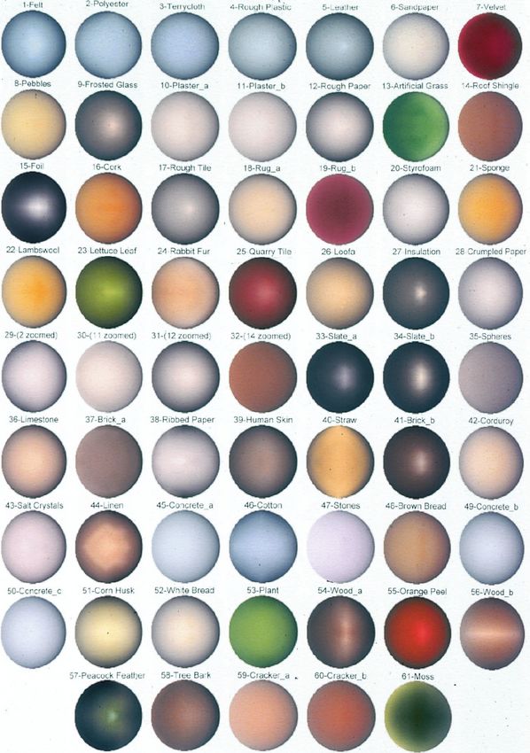
2      •     K. J. Dana et al.

Additional Key Words and Phrases: Bidirectional reflectance distribution function, bidirec-
tional texture function, “3D texture”

1. INTRODUCTION
Characterizing the appearance of real-world textured surfaces is a funda-
mental problem in computer vision and computer graphics. Appearance
depends on view, illumination, and the scale at which the texture is
observed. At coarse scale, where local surface variations are subpixel and
local intensity is uniform, appearance is characterized by the BRDF (bidi-
rectional reflectance distribution function). At fine scale, where the surface
variations give rise to local intensity variations, appearance can be charac-
terized by the BTF (bidirectional texture function). As a direct analogy to
the BRDF, we have introduced the term BTF to describe the appearance of
texture as a function of illumination and viewing direction. Specifically, the
BTF is a texture image parameterized by the illumination and viewing
angles. This taxonomy is illustrated in Figure 1.
   Studying the dependence of texture on viewing and illumination direc-
tions is fairly new in texture research and so there is only a limited amount
of related work. For example, Koenderink and van Doorn [1996] discuss the
issues involved in texture due to surface geometry, Stavridi et al. [1997]
measure the variation of brick texture with imaging conditions, Debevec et
al. [1996] incorporate a type of view-dependent texture for rendering
architecture and Leung and Malik [1997] consider perpendicular texture
comprised of elements normal to the surface. Our work in addressing the
problem has resulted in two publicly available databases: a BTF measure-
ment database with texture images from over 60 different samples, each
observed with over 200 combinations of viewing and illumination directions
and a BRDF measurement database with reflectance measurements from
the same 60 samples. Each of these databases is made publicly available at
www.cs.columbia.edu/CAVE/curet. In this article, we provide a detailed
description of the database contents and measurement procedure. The
database has generated substantial interest since it first became available
[Dana et al. 1996]. This interest is evident in the numerous works using the
database: BRDF model-fitting in Dana et al. [1996, 1997] and Koenderink
et al. [1998], histogram simulations in Ginneken et al. [1997], a histogram
model and histogram model-fitting in Dana and Nayar [1998], and SVD
(singular value decomposition) analysis in Suen and Healey [1998].
   The BTF database, comprised of over 14,000 images, can be used for
development of 3-D texture algorithms. In computer graphics, traditional
methods of 2-D texture synthesis and texture-mapping make no provision
for the change in texture appearance with viewing and illumination direc-
tions. For example, in 2-D texture-mapping when a single digital image of a
rough surface is mapped onto a 3-D object, the appearance of roughness is
usually lost or distorted. Bump-mapping [Blinn 1977, 1978; Becker and
ACM Transactions on Graphics, Vol. 18, No. 1, January 1999.
Reflectance and Texture           •      3

Fig. 1. Taxonomy of surface appearance. When viewing and illumination directions are fixed,
surface appearance can be described by either reflectance (at coarse-scale observation) or
texture (at fine-scale observation). When viewing and illumination directions vary, the
equivalent descriptions are the BRDF and the BTF. Analogous to the BRDF, BTF is a function
of four independent angles (two each for viewing and illumination directions).

Max 1993] preserves some of the appearance of roughness, but knowledge
of the surface shape is required and shadows cast from the local surface
relief are not rendered. Many of the problems associated with traditional
texture-mapping and bump-mapping techniques are described in Koen-
derink and van Doorn [1996]. If the exact geometry of the surface is known,
ray tracing can be used but at a high computational cost. Another method
of rendering surface texture is solid texturing,1 which combines a volumet-
ric texture synthesis with volume rendering techniques. This method is
computationally intensive and is applicable for a limited variety of tex-
tures. With the availability of the BTF database, the potential exists for
3-D texturing algorithms using images, without the need for a volumetric
texture model or surface synthesis procedure.
   In computer vision, current texture algorithms such as shape-from-texture,
texture segmentation, and texture recognition are appropriate for textures
that arise from albedo or color variations on smooth surfaces.2 In contrast, the
texture due to surface roughness has complex dependencies on viewing and
illumination directions. These dependencies cannot be studied using existing
texture databases that include few images or a single image of each sample
(for instance, the widely used Brodatz database). Our texture database covers
a diverse collection of rough surfaces and captures the variation of image
texture with changing illumination and viewing directions. This BTF database
is a first step towards extending current texture analysis algorithms to include
texture from nonsmooth real-world surfaces.
   Although the BTF is a new framework for the study of texture, the BRDF
has been around for decades. The BRDF was first defined in 1970 by
Nicodemus [1970] and Nicodemus et al. [1977] as the scattered surface
radiance (in units of watts per unit area per unit solid angle) divided by the
incident surface irradiance (in units of watts per unit area). Interest in
measuring the BRDF spans many fields including optical engineering,
remote-sensing, computer vision, and computer graphics. In optical engi-

1
 Please see Peachey [1985], Perlin [1989, 1985], Lewis [1989], and Sakas and Kernke [1994].
2
 Please see Chatterjee [1993], Kashyap [1984], Krumm and Shafer [1995], Patel and Cohen
[1992], Super and Bovik [1995], Wang and Healey [1996], and Xie and Brady [1996].

                                      ACM Transactions on Graphics, Vol. 18, No. 1, January 1999.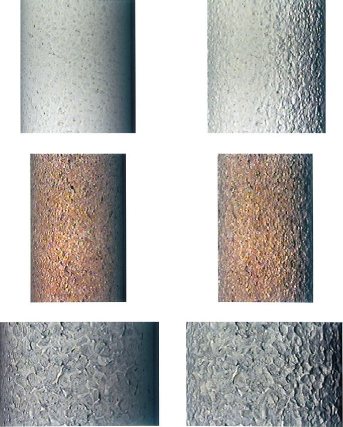
4      •     K. J. Dana et al.

neering, the BRDF of components is a critical design issue. Optical scatter
is considered a source of noise that limits system resolution and throughput
[Stover 1989]. In the development of space optics, scatter from contami-
nants (such as rocket exhaust) is a key issue in system development [Stover
1989; Herren 1989; Howard et al. 1989]. In other fields, the BRDF is
needed not to measure contamination of simple optical surfaces, but rather
to understand the inherently complex optical behavior of natural surfaces.
In remote-sensing, the BRDF of terrestrial surfaces such as soil, vegeta-
tion, snow, and ice is a popular research topic.3 Here, there is a need to
distinguish changes in imaging parameters from changes due to target
variations (different soil type, change in vegetation, change in soil mois-
ture, etc.). In computer vision, the reflectance from a surface can be used to
determine 3-D shape such as in shape-from-shading [Horn and Brooks
1989] or photometric stereo [Woodham 1980]. In order for such algorithms
to function properly, the BRDF must be well modeled which can be verified
via measurement. In computer graphics, the BRDF has a clear application
in the rendering of realistic surfaces.
   Although BRDF models have been widely discussed and used in com-
puter vision and computer graphics,4 the BRDFs of a large and diverse
collection of real-world surfaces have never before been available. Our
measurements comprise a comprehensive BTF/BRDF database (the first of
its kind) that is now publicly available. Our measurement procedure does
not employ a gonioreflectometer or the hemispherical mirror arrangement
described in Ward [1992]. Instead, a robotic manipulator and CCD camera
are employed to allow simultaneous measurement of the BTF and the
BRDF of large samples (about 10 3 10 cm). Exactly how well the BRDFs of
real-world surfaces fit existing models has remained unknown as each
model is typically verified using a small number (two to six) of surfaces.
Our large database allows researchers to evaluate the performance of
existing and future BRDF models and representations.

2. MEASUREMENT METHODS

2.1 Measurement Device
Our measurement equipment depicted in Figure 2 is comprised of a robot,5
lamp,6 personal computer,7 photometer,8 and video camera.9 Measuring the

3
  Please see Sandmeier et al. [1995], Nolin et al. [1994], Li et al. [1994], and Schluessel et al.
[1994].
4
  Please see Westin et al. [1992], Torrance and Sparrow [1967], Poulin and Fournier [1990],
Ward [1992], Nayar et al. [1991], Tagare and DeFigueiredo [1993], Wolff [1994], Koenderink et
al. [1996, 1998], Oren and Nayar [1995], and van Ginneken et al. [1998].
5
  SCORBOT-ER V by ESHED Robotec (Tel Aviv, Israel).
6
  Halogen bulb with a Fresnel lens.
7
  IBM compatible PC running Windows 3.1 with “Videomaker” frame grabber by VITEC
Multimedia.
8
  SpectraScan PR-704 by Photoresearch (Chatsworth, CA).
9
  Sony DXC-930 3-CCD color video camera.

ACM Transactions on Graphics, Vol. 18, No. 1, January 1999.
Reflectance and Texture           •      5

Fig. 2. Measurement setup. The equipment consists of a personal computer with a 24-bit
RGB frame grabber, a robot arm to orient the texture samples, a halogen bulb with a Fresnel
lens which produces a parallel beam, a photometer, and a 3-CCD color video camera (not
shown).

BRDF requires radiance measurements for a range of viewing/illumination
directions. For each sample and each combination of illumination and
viewing directions, an image from the video camera is captured by the
frame grabber. These images have 640 3 480 pixels with 24 bits per pixel
(8 bits per RGB channel). The pixel values are converted to radiance values
using a calibration scheme described in Section 2.3. The calibrated images
serve as the BTF measurements and these images are averaged over the
sample area to obtain the BRDF measurements, as illustrated in Figure 3.
   The need to vary the viewing and light source directions over the entire
hemisphere of possible directions presents a practical obstacle in the
measurements. This difficulty is reduced considerably by orienting the
sample to generate the varied conditions. As illustrated in Figure 4, the
light source remains fixed throughout the measurements. The light rays
incident on the sample are approximately parallel and uniformly illumi-
nate the sample. The camera is mounted on a tripod and its optical axis is
parallel to the floor of the lab. During measurements for a given sample,
the camera is moved to seven different locations, each separated by 22.5
degrees in the ground plane at a distance of 200cm from the sample. For
each camera position, the sample is oriented so that its normal is directed
toward the vertices of the facets that tessellate the fixed quarter-sphere
illustrated in Figure 4.10 With this arrangement, a considerable number of
measurements are made in the plane of incidence (i.e., illumination direc-
tion, viewing direction, and sample normal lie in the same plane). Also, for
each camera position, a specular point is included where the sample normal
bisects the angle between the viewing and illumination directions. Sample
orientations with corresponding viewing angles or illumination angles
greater than 85 degrees are excluded from the measurements to avoid
self-occlusion and self-shadowing. This exclusion results in the collection of
205 images for each sample with 55 images taken at camera position 1, 48

10
  The vertices of the quarter sphere shown in Figure 4(a) were obtained by starting with the
two triangles formed by the coordinates (1,0,0), (0,0,1),(0,21,0), and (0,1,0) and then barycen-
trically subdividing.

                                        ACM Transactions on Graphics, Vol. 18, No. 1, January 1999.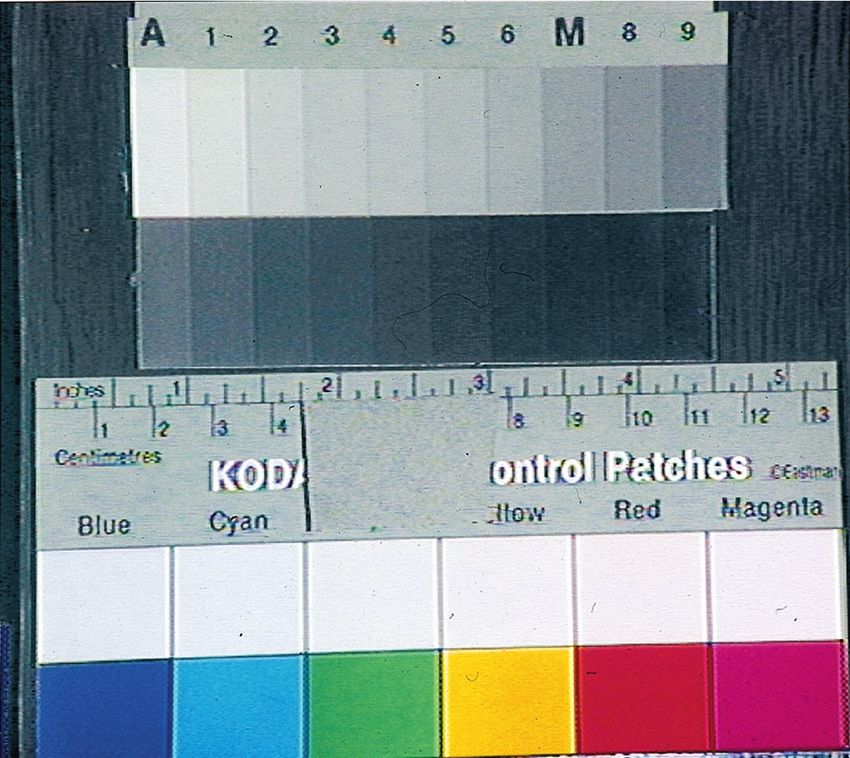
6      •     K. J. Dana et al.

Fig. 3. Sample (roofing shingle) mounted on a robot. The average intensity over the sample is
the radiance or BRDF measurement and the image of the sample is the texture or BTF
measurement for a particular viewing and light source direction.

Fig. 4. The vertices on the hemisphere correspond to the directions to which the robot orients
the sample’s surface normal. The illumination direction remains fixed and the camera is
positioned in seven different locations in a plane. These seven locations correspond to angular
deviations of 22.5°, 45°, 67.5°, 90°, 112.5°, 135°, 157.5° from the light source direction. For
each camera position, images of the sample are acquired at the subset of sample orientations
that are visible and illuminated. The total number of images acquired per sample is 205.

images at position 2, 39 images at position 3, 28 images at position 4, 19
images at position 5, 12 images at position 6, and 4 images at position 7. A
complete table of sample orientations is given in the online database.
   Figure 5 shows an alternative representation of the 205 measurements
for each sample. Here, the illumination directions are shown in the sample
coordinate frame xs–ys–zs. Notice that the illumination directions are
evenly distributed over the quarter-sphere so the set of all possible illumi-
nation directions is well represented by the subset used in the measure-
ments. To determine which viewing directions are paired with each of these
illumination directions, consider that each distinct illumination direction
corresponds to a distinct sample orientation. Consequently, there are a
maximum of seven viewing directions for each illumination direction,
corresponding to the seven camera positions. There can be less than seven
viewing directions for a given illumination direction because a particular
combination of sample orientation and camera position is excluded if the
corresponding viewing direction is greater than 85 degrees from the sample
ACM Transactions on Graphics, Vol. 18, No. 1, January 1999.
Reflectance and Texture           •      7

Fig. 5. An alternative interpretation of the measurements described in Figure 4. Illumina-
tion directions are shown in the sample coordinate frame. The sample lies in the xs–ys plane
and its global normal points in the direction of zs. Each circular marker represents a distinct
illumination direction. For each of these illumination directions, the sample is imaged from
seven viewing directions, corresponding to the seven camera positions shown in Figure 4.

normal. Figure 6 shows examples of illumination directions with their
associated viewing directions.
  For anisotropic textures, the 205 measurements are repeated after rotat-
ing the sample about zs by either 90 degrees or 45 degrees depending on
the structure of the anisotropy. For example, the linen sample was rotated
by 45 degrees because its horizontal and vertical threadings form a gridlike
structure that does not change when rotated by 90 degrees. On the other
hand, the sample of corduroy was rotated by 90 degrees to obtain the
maximum difference in surface structure. The anisotropic textures were
Sample 38 (ribbed paper), Sample 40 (straw), Sample 42 (corduroy), Sam-
ple 44 (linen), Sample 46 (cotton), Sample 51 (corn husk), Sample 54
(wood_a), Sample 56 (wood_b), and Sample 58 (tree bark).

2.2 Samples for Measurements
The collection of real-world surfaces used in the measurements is illus-
trated in Figure 7. Samples of these surfaces were mounted on 10 3 12cm
bases that were constructed to fit onto the robot gripper. Each sample,
though globally planar, exhibits considerable depth variation or macro-
scopic surface roughness. The samples were chosen to span a wide range of
geometric and photometric properties. The categories include specular
surfaces (aluminum foil, artificial grass), diffuse surfaces (plaster, con-
crete), isotropic surfaces (cork, leather, styrofoam), anisotropic surfaces
(straw, corduroy, corn husk), surfaces with large height variations (crum-
pled paper, terrycloth, pebbles), surfaces with small height variations
(sandpaper, quarry tile, brick), pastel surfaces (paper, cotton), colored
surfaces (velvet, rug), natural surfaces (moss, lettuce, fur) and manmade
surfaces (sponge, terrycloth, velvet).
                                       ACM Transactions on Graphics, Vol. 18, No. 1, January 1999.
8 • K. J. Dana et al.
Fig. 6. Viewing directions in the sample coordinate frame. For each illumination direction
shown in Figure 5, there are at most seven associated viewing directions corresponding to the
seven camera positions. Each panel shows an example of an illumination direction (dotted
line) and the associated viewing directions (solid lines). The viewing directions lie in a plane
that changes with illumination direction. Since the sample is not visible for every camera
position, the number of associated viewing conditions also varies with illumination direction.
The plots show examples of illumination directions with two to seven associated viewing
directions.
2.3 Radiometric Calibration
Radiometric calibration is performed to interpret pixel values as radiance.
This calibration is done by measuring radiance from the samples and from
a Kodak standard card11 (illustrated in Figure 8) using a photometer.12 We
refer to the radiance measurements and pixel values from the Kodak
standard card as the standard calibration data. The radiance measure-
ments and pixel values from the sample are termed sample calibration data.
2.3.1 Standard Calibration Data. To obtain the standard calibration
data, the standard card shown in Figure 8 is placed in the robotic sample
holder. The card has 20 gray strips with 0.1 density increments and
relative density values from a nominal “white” of approximately 0.05 (90%
reflectance) to 1.95 (1% reflectance). In addition, the card has 12 colored-
strips with two shades of blue, cyan, green, yellow, red, and magenta. The
11
Kodak Color Separation Guide and Gray Scale, Kodak Publication No. Q-13.
12
SpectraScan PR-704 by Photoresearch (Chatsworth, CA).
ACM Transactions on Graphics, Vol. 18, No. 1, January 1999.Reflectance and Texture • 9
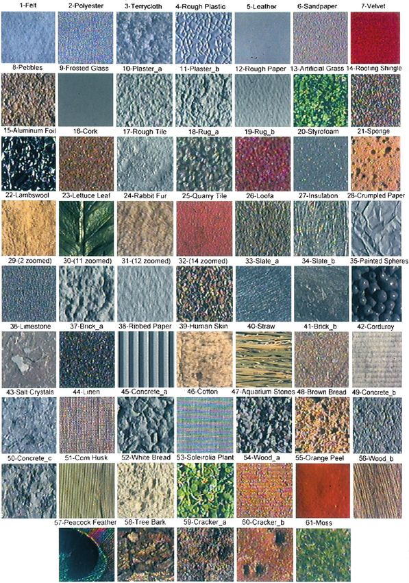
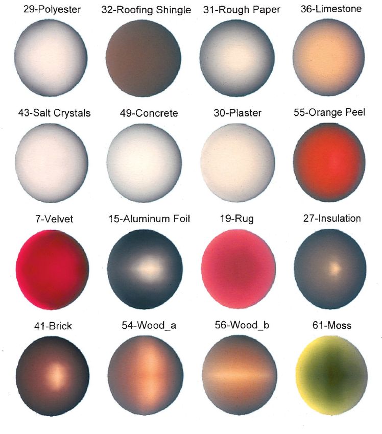
Fig. 7. The collection of 61 real-world surfaces used in the measurements. The name and
number of each sample is indicated above its image. The samples were chosen to span a wide
range of geometric and photometric properties. Different samples of the same type of surfaces
are denoted by letters, for example, Brick_a and Brick_b. Samples 29, 30, 31, and 32 are
close-up views of samples 2, 11, 12, and 14, respectively.
ACM Transactions on Graphics, Vol. 18, No. 1, January 1999.10 • K. J. Dana et al.
Fig. 8. Kodak standard card with 20 strips of gray and 12 color strips.
sample holder is oriented so that the card is frontal to the lamp. The
photometer is placed in camera position 1, 22.5° from the lamp as illus-
trated in Figure 4. The photometer has a circular region of interest (0.8cm
in diameter) marked in its viewfinder to identify the position on the card
from which the radiance is measured. To obtain the standard calibration
data, the photometer is oriented so that its region of interest is positioned
within each strip on the standard card. The photometer records 200
radiance values, corresponding to the radiance in watts/(steridian 2
meter2) for each 2nm interval between the wavelengths 380nm and 780nm.
The recording of radiance values from the standard card does not have to
be done for every day of the measurement procedure. In theory, the
radiance need only be measured once for each lamp used in the experiment.
However, to keep track of the slowly decreasing intensity of a particular
lamp over the course of the experiment, the recordings were made more
than once for each lamp. See Appendix A for a discussion.
To relate radiance to pixel values, an image of the standard card must be
obtained as well. Since the camera settings can vary for each sample, an
image of the standard card is obtained for every sample measured. After
the lens aperture and camera settings are adjusted for each sample, the
image of the standard card is recorded. The pixels in each strip (isolated by
manual segmentation) are averaged. Since there are 32 strips on the card
(20 gray and 12 color), the standard calibration data are 32 radiance values
with corresponding pixel values.
ACM Transactions on Graphics, Vol. 18, No. 1, January 1999.Reflectance and Texture • 11
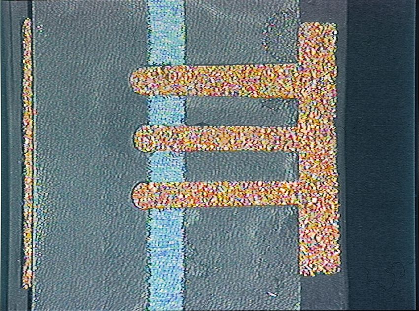
Fig. 9. Fiducial marker attached to sample. This metallic grid with painted stripe is used as
a fiducial marker to specify a spatial region for measuring radiance with the photometer and
recording pixel values with the video camera. These radiance and pixel measurements are
used in radiometric calibration.
2.3.2 Sample Calibration Data. Sample calibration data (i.e., radiance
and pixel values taken from the sample) are useful because calibration is
likely to be wavelength dependent. That is, the relationship between
radiance and pixel values is likely to depend on the wavelength of interest.
Since the wavelength of interest is determined by the color of the sample, it
makes sense to calibrate using reflectance values from the sample. Stan-
dard calibration data are used in conjunction with sample calibration data
because the standard calibration data often cover the range of the operat-
ing curve better than the sample calibration data especially in the case of
dark samples.
To determine the relationship between radiance and pixel values an
operating curve is needed, where the radiance and pixel values are re-
corded over a range of reflected intensity. For the standard calibration
data, this range of measurements was obtained via the varying reflectance
values of the gray reference strips. For the sample data we varied the angle
between the light source and the sample normal (keeping the sample
normal in the plane of incidence) to obtain a range of bright and dark
intensity values.
When recording the sample calibration data, a fiducial marker is neces-
sary to localize the region where pixel values and photometer readings are
obtained. We use a metal grid that fits over the sample as the fiducial
marker, as illustrated in Figure 9. The circular photometer region (0.8cm
diameter) is positioned so that its center diameter aligns with the right
edge of the grid line. For eight sample orientations, three radiance and
ACM Transactions on Graphics, Vol. 18, No. 1, January 1999.12 • K. J. Dana et al.
pixel values are obtained corresponding to the three slit openings of the
grid. The eight sample orientations correspond to the light source direction
and the directions of camera positions 1 through 7. These orientations were
chosen so that bright and dark points would be included in the sample
calibration data.
We use two methods for radiometric calibration. In both methods the
relationship between radiance and associated pixel value is approximated
as linear. The first method, termed gray calibration, relates the average of
the red, green, and blue pixels to the total radiance recorded by the
photometer (i.e., radiance from the wavelength range 380nm to 780nm).
Letting r denote the total radiance and p denote the average pixel value,
the parameters estimated are a and b where
r 5 a p p 1 b. (1)
The gray calibration results are illustrated in Figure 19 of Appendix C.
The second method, termed color calibration, estimates the camera
sensitivity curves for the red, green, and blue CCD of the video camera. The
average radiance for the red, green, and blue spectral regions is obtained
by integrating the estimated sensitivity curves multiplied by the radiance
per wavelength (as measured by the photometer). The relationship between
the RGB pixels and the corresponding RGB radiance is assumed linear. The
sensitivity function is assumed to be a unit area Gaussian function. For
each sample, the mean and variance of this Gaussian function is estimated
along with the linear radiometric calibration curves through nonlinear
estimation. The resulting mean and variances over all samples are aver-
aged to obtain the final estimates of the sensitivity curves. These estimated
sensitivity curves, depicted in Figure 10, were used to obtain the final
estimate for the linear relationships between the RGB pixel values and
RGB radiance for each sample. Let r r , r g , and r b denote the red, green, and
blue radiance, respectively, and let p r , p g , and p b denote the red, green,
and blue pixel values, respectively. Then the color calibration method
estimates a r , b r , a g , b g , a b , and b b , where
rr 5 ar p pr 1 br , (2)
rg 5 ag p pg 1 bg , (3)
rb 5 ab p pb 1 bb . (4)
The color calibration results are illustrated in Figure 20 of Appendix C.
In both the gray and color calibration methods the data are not always
weighted equally. Sample calibration data are weighted more than the
standard calibration except when the sample calibration data suffer from
underflow or overflow. Data with significant pixel underflow (pixel values
near zero) or overflow (pixel values near 255) are not used.
ACM Transactions on Graphics, Vol. 18, No. 1, January 1999.Reflectance and Texture • 13
Fig. 10. The estimated sensitivity curve for the 3-CCD color video camera. The mean and
standard deviation for the red sensitivity curve were 604nm and 16.6nm, respectively. The
mean and standard deviation for the green sensitivity curve were 538nm and 29.2nm,
respectively. The mean and standard deviation for the red sensitivity curve were 460nm and
17nm, respectively. Note that each estimated sensitivity curve is normalized to have unit area.
2.4 Measurement Procedure
The general steps of the measurement procedure have been discussed in
previous sections. The purpose of this section is to clarify the procedure by
listing the steps in chronological order as follows.
Adjust camera aperture. Place camera in Position 1 and place current
sample in sample holder on robotic manipulator. Orient sample so that it
appears very bright (for most samples this will occur either in a position
frontal to the lamp or a specular position) and adjust the aperture to
minimize pixel overflow. Orient the sample so that it appears quite dark
(e.g., at an orientation far from the light source direction) and adjust the
aperture to reduce pixel underflow. This process is repeated until a
reasonable aperture size for the current sample is obtained. Pixel overflow
and underflow are rarely eliminated completely and contribute to the
sources of error as discussed in Appendix B.
Record a reference image of gray card. The sample is replaced with a
Kodak 18% gray card13 cut to sample size (10 3 12cm). An image of this
card is recorded with the card frontal to the illumination and the camera in
Position 1. These data are used to evaluate the spatial uniformity of the
illumination as discussed in Appendix A.
Record standard calibration data (pixel values). Replace Kodak 18%
gray card with the Kodak standard card shown in Figure 8. Record an
image with the sample holder oriented frontal to the lamp and the camera
in Position 1.
13
Kodak Gray Cards, Kodak Publication No. R-27.
ACM Transactions on Graphics, Vol. 18, No. 1, January 1999.14 • K. J. Dana et al. Record sample calibration data. Replace standard card with sample and place grid (fiducial marker) on sample as shown in Figure 9. Record eight images corresponding to the sample oriented toward the light source and in the direction of the seven camera positions. Replace camera with photometer in Position 1 and record the radiance values for each of the three marked positions on the sample and for each of the eight orientations of the sample. Record sample images for camera in Position 1. Replace photometer with camera, remove grid from sample. Take all measurements needed for the camera in Position 1 (this stage, which consists of alternate steps of reorienting the sample and recording the image, is done automatically). Move camera and record sample images for camera in Position 2. Repeat for all seven camera positions. Repeat measurements for anisotropic samples. For anisotropic samples, rotate the sample about its normal (by either 45 or 90 degrees depending on the structure) and record another 205 samples over the seven camera positions. Get radiance measurements for calibration. Occasionally do a lamp calibration which requires getting photometer readings for the 18% gray card and 32 strips on the standard card. The measured radiance from the 18% gray card is used to estimate the irradiance for each lamp as discussed in the normalization step of Section 2.5. Note that the camera and photometer switch positions several times and at first glance it may seem that reordering the steps of the procedure would reduce this problem. However, the particular ordering of steps as listed is necessary. For instance, the aperture must be set with no grid on the sample (because the grid reduces overall brightness) and the grid cannot be removed between photometer and camera measurements (otherwise the fiducial markers would move). 2.5 Postprocessing Here are the main steps in postprocessing. Calibration. Transform pixel values to radiance as described in Section 2.3. Segmentation. Segmentation simply requires identifying the part of the image in which the sample resides. Such segmentation is necessary so that the region for averaging can be identified for computing the BRDF. This is done by manually clicking on a subset of the corner points and using those values (along with the known sample orientation in each image and an orthographic projection assumption) to compute the transformations neces- sary to find the corner points of all the images in the sample measurement set. The resulting corner sets are manually inspected and adjusted when necessary to ensure that no background pixels are included in the measure- ments. ACM Transactions on Graphics, Vol. 18, No. 1, January 1999.
Reflectance and Texture            •      15

   Normalization. An irradiance estimate is obtained using the radiance
measured from the 18% Lambertian gray card. Specifically, the irradiance
is the measured radiance multiplied by the factor p/0.18. Normalization by
this estimated irradiance enables a BRDF estimate to be computed from
the radiance values.

3. TEXTURE MEASUREMENTS

3.1 BTF Database
The appearance of a rough surface, whether manifested as a single radi-
ance value or as image texture, depends on viewing and illumination
directions. Just as the BRDF describes the coarse-scale appearance of a
rough surface, the BTF (bidirectional texture function) is useful for describ-
ing the fine-scale appearance of a rough surface. Our measurements of
image texture comprise the first BTF database for real-world surfaces. The
database has over 14,000 images (61 samples, 205 measurements per
sample, 205 additional measurements for anisotropic samples).
   To illustrate the use of the BTF representation, Figure 11 shows ren-
dered cylinders of plaster, pebbles, and concrete using two methods:
ordinary 2-D texture-mapping and 3-D texture-mapping using the BTF
measurement. Figure 12 shows similar renderings with crumpled paper,
plush rug, and wood. The phrase “2-D texture-mapping” is used to refer to
the warping or mapping of a single texture image onto an arbitrarily
shaped object. For the 2-D texture-mapping examples in Figures 11 and 12,
the texture image is taken as the frontally viewed image with the illumina-
tion direction at an angle of 22.5° to the right. For the 3-D texture-mapping
examples in Figures 11 and 12, 13 images per sample are used from the
database collection of 205 images. Of these 13 images, one view is the
frontal view and the rest are oblique views of the sample. More specifically,
these 13 images correspond to orientations of the sample’s global surface
normal in the plane of the viewing and illumination direction at intervals
of 11.25 degrees with the camera in Position 1 (see Figure 4). We make a
piecewise planar approximation of the cylinder so that each planar section
corresponds to the viewing and illumination direction of one of the 13
images. Then a section of each image is pasted in its appropriate position
with averaging of three pixels at the section borders to reduce the appear-
ance of seams.
   Clearly 2-D texture-mapping, as we have defined it, cannot account for
the variations in texture appearance due to local shading, foreshortening,
shadowing, occlusions, and interreflections. These complex photometric and
geometric effects significantly change the appearance of the surface tex-
ture. By using several images for 3-D texture-mapping of the cylinder, we
can incorporate these effects and substantially improve the image realism.
Consider the renderings shown in Figures 11 and 12. The surface rough-
ness of the cylinders rendered with 3-D texture-mapping is readily appar-
ent, whereas the cylinders rendered with 2-D texture-mapping appear
rather smooth.
                                ACM Transactions on Graphics, Vol. 18, No. 1, January 1999.
16 • K. J. Dana et al. Fig. 11. Cylinders rendered with 2-D texture-mapping (left) and 3-D texture-mapping (right). From top to bottom, the samples rendered are Sample 11 (plaster), Sample 8 (pebbles), and Sample 45 (concrete). These rendered cylinders demonstrate the potential of 3-D texture- mapping, but there are many unresolved issues. For instance, interpolation must be done between measured BTF images. Also, seams become a problem when the sizes of the characteristic texture elements become large ACM Transactions on Graphics, Vol. 18, No. 1, January 1999.
Reflectance and Texture • 17
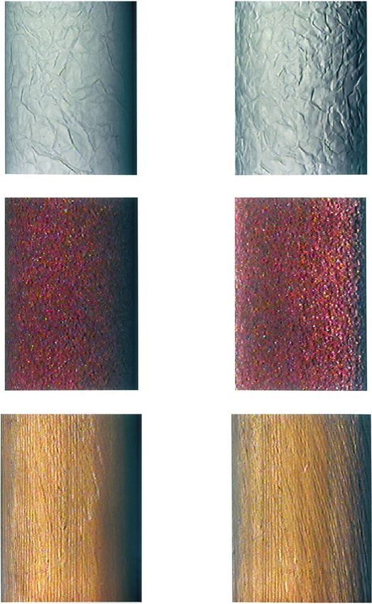
Fig. 12. Cylinders rendered with 2-D texture-mapping (left) and 3-D texture-mapping (right).
From top to bottom, the samples rendered are Sample 28 (crumpled paper), Sample 19 (plush
rug), and Sample 56 (wood).
ACM Transactions on Graphics, Vol. 18, No. 1, January 1999.18 • K. J. Dana et al. Fig. 13. Changes in the spatial spectrum due to changes in imaging conditions. (Top row) Two images of Sample 11 with different illumination and viewing directions. (Bottom row) Spatial spectrum of the images in the top row, with zero frequency at the center and brighter regions corresponding to higher magnitudes. The orientation change in the spectrum is due to the change of illumination direction which causes a change in the shadow direction. compared to the size of the patch being textured. The database presented here is a starting point for further exploration into this area. Important observations of the spatial–spectral content of image texture can be made using the BTF database. Consider the same sample shown under two different sets of illumination and viewing directions in Figure 13. The corresponding spatial Fourier spectra are also shown in Figure 13. Notice that the spectra are quite different. Most of the difference is due to the change in azimuthal angle of the illumination direction which causes a change in the shadowing direction and hence a change in the dominant orientation of the spectrum. If the image texture were due to a planar albedo or color variation, changes in the illumination direction would not have this type of effect on the spectrum. Source direction changes would only cause a uniform scaling of the intensity over the entire image. These observations have important implications in computer vision because tex- ture recognition algorithms are often based on the spectral content of image textures. For recognition of real-world surfaces, invariant of illumination, and viewing direction, the BTF must be considered. ACM Transactions on Graphics, Vol. 18, No. 1, January 1999.
Reflectance and Texture            •      19

4. BRDF MEASUREMENTS

4.1 Comparison with Other BRDF Measurement Systems
BRDF measurement systems come in a wide variety of sizes and configura-
tions. In the field of optical engineering, the apparatus is designed to
measure effects of microscopic roughness from contaminants and thus the
field of view can be quite small. For remote-sensing, the surface unit
measured can be quite large as the systems are designed to measure large
patches of terrestrial surfaces [Sandmeier et al. 1995]. Our system is
designed to operate in a range that is useful for measuring the variety of
surfaces that are of interest in computer graphics. As mentioned, the
surface patch over which the BRDF is computed is approximately 10 3
12cm and planar samples of this size for the variety of real-world surfaces
shown in Figure 7 are relatively easy to obtain. Images of this size are
sufficiently large to capture the characteristic surface variations of the
texture of each of these surfaces.
   The components of the BRDF measurement system vary also. The type of
light sources varies from system to system and is often either a halogen
source [Stavridi et al. 1997; Ward 1992] or a laser source [Marx and
Vorburger 1989]. In some cases polarized light is used [Betty et al. 1996].
In some systems, mirrors are used to orient the incoming light [Marx and
Vorburger 1989; Betty et al. 1996]. In other systems, especially when the
sample must stay fixed (as in measurement of terrain for remote-sensing),
a goniometer is used to orient the light source and detector [Sandmeier et
al. 1995]. A goniometer consists of two arcs with a varying azimuth angle,
one for the detector and one for the light source (if an artificial light source
is used). In most cases the detector is some type of photometer, but in some
apparatus, the detector is a CCD camera [Ward 1992; Karner et al. 1996].
One system allows the simultaneous capture of the hemisphere of scatter-
ing directions by using a hemispherical mirror and a fish-eye lens [Ward
1992].
   Our measurement apparatus is driven by the goal of also measuring
bidirectional texture. To achieve that goal, a CCD camera is our main
sensor element. Some of the sources of error in our procedure (see Appendix
B) are attributable to the imperfect calibration of CCD pixel to radiance
values. Therefore other BRDF measurement systems may have better
accuracy. However our system’s simplicity and its suitability for simulta-
neous BRDF and BTF measurements make it ideal for our purposes.
   Variations of BRDF measurement techniques as described and observa-
tion of sources of error among different BRDF measurements led to the
development of the ASTM standard [ASTM]. For a discussion of our BRDF
measurement apparatus and method in the context of the ASTM standard,
see Appendix E.

4.2 BRDF Database
The BRDF measurements form a database with over 14,000 reflectance
measurements (61 samples, 205 measurements per sample, 205 additional
                                 ACM Transactions on Graphics, Vol. 18, No. 1, January 1999.
20 • K. J. Dana et al. measurements for anisotropic samples). This entire set is available elec- tronically. The measured BRDFs are quite diverse and reveal the complex appearance of many ordinary surfaces. Figures 14 and 15 illustrate examples of spheres rendered with the measured BRDF as seen from camera position 1, that is, with illumination from 22.5° to the right. Interpolation is used to obtain a continuous radiance pattern over each sphere. The rendered sphere corresponding to velvet (Sample 7) shows a particularly interesting BRDF that has bright regions when the global surface normal is close to 90 degrees from the illumination direction. This effect can be accounted for by considering the individual strands comprising the velvet structure that reflect light strongly as the illumination becomes oblique. This effect is consistent with the observed brightness in the interiors of folds of a velvet sheet. Indeed, the rendered velvet sphere gives a convincing impression of velvet. The rendered spheres of plaster (Sample 30) and roofing shingle (Sample 32) show a fairly flat appearance which is quite different from the Lamber- tian prediction for such matte objects, but is consistent with Nayar and Oren [1995] and Oren and Nayar [1995]. Concrete (Sample 49) and salt crystals (Sample 43) also show a somewhat flat appearance, whereas rough paper (Sample 31) is more Lambertian. The plush rug (Sample 19) and moss (Sample 61) have similar reflectance patterns as one would expect from the similarities of their geometry. Rendered spheres from two aniso- tropic samples of wood (Sample 54 and Sample 56) are also illustrated in Figures 14 and 15. The structure of the anisotropy of sample 54 consists of horizontally oriented ridges. This ridge structure causes a vertical bright stripe instead of a specular lobe in the rendered sphere. Sample 56 shows a similar effect, but the anisotropic structure for this sample consists of near vertical ridges. Consequently, the corresponding rendered sphere shows a horizontal bright region due to the surface geometry. 5. ADDITIONAL INFORMATION The BRDF measurements and BTF texture images are too numerous for inclusion in this article. The website (www.cs.columbia.edu/CAVE/ curet) serves as a complement to this article and readers can access both databases electronically. 6. IMPLICATIONS FOR GRAPHICS Our BRDF and BTF measurement databases together represent an exten- sive investigation of the appearance of real-world surfaces. Each of these databases has important implications for computer graphics. Our BTF measurement database is the first comprehensive investigation of texture appearance as a function of viewing and illumination directions. As illustrated in Figures 11 and 13, changes of view and illumination cause notable effects on texture appearance that are not considered by current texture rendering algorithms. When the surface is rough, standard texture rendering tends to be too flat and unrealistic. Even if the rendering from a ACM Transactions on Graphics, Vol. 18, No. 1, January 1999.
Reflectance and Texture            •      21

Fig. 14. Spheres rendered using the BRDF measurements obtained from camera position 1
(illumination at 22.5° to the right). Interpolation was used to obtain radiance values between
the measured points.

                                       ACM Transactions on Graphics, Vol. 18, No. 1, January 1999.
22 • K. J. Dana et al. Fig. 15. Enlarged view of selected spheres (from Figure 14) rendered using the BRDF measurements obtained from camera position 1 (illumination at 22.5° to the right). Interpola- tion was used to obtain radiance values between the measured points. single view is suitably realistic, the realism is lost when the view or illumination changes. The database illustrates the need for 3-D texture rendering algorithms and serves as a starting point for their exploration. Our BRDF measurement database provides a thorough investigation of the reflectance properties of real-world rough surfaces. This database fills a long-standing need for a benchmark to test and compare BRDF models as ACM Transactions on Graphics, Vol. 18, No. 1, January 1999.
Reflectance and Texture            •      23

we have done in Dana et al. [1997] for the Oren–Nayar [1995] model and
the Koenderink et al. [1996] decomposition. Such a comparison is useful in
choosing a representation that has the right balance of accuracy and
compactness for the application at hand. In circumstances that necessitate
the use of a less accurate reflectance model, such as the Lambertian model,
the database provides a means of gauging expected errors.

APPENDIX A. Light Sources
Because of the limited lifetime of the lamps employed in the measure-
ments, three different lamps were used:
—Lamp 1 was used for Samples 1– 8.
—Lamp 2 was used for Samples 9 – 44.
—Lamp 3 was used for Samples 45– 61.
Each of these lamps was operated with a regulated power supply.
   Periodically during the measurements we performed a lamp calibration
which consisted of placing the photometer region of interest over each strip
on the Kodak standard card. This card consisted of 20 gray strips (strip no.
0 –19), a piece of a standard 18% gray card (strip no. 20) that was attached
at the center of the card, and 12 color strips (strip no. 21–32). The main
purpose of these lamp calibrations was to relate pixel values to radiance
values as described in Section 2.3. (An image of the Kodak standard card
was obtained for each sample after the camera aperture was set). The
second purpose of the lamp calibrations was to determine the temporal
stability of the lamp (whether it remained at approximately the same
brightness for each day of the experiment).
   For lamp 1, two calibrations were performed on Day 1 and Day 4 of the
measurements. Sample 1 was measured on Day 1 and sample 8 was
measured on Day 4. Figure 16 shows the 33 photometer measurements
from the standard calibration card for each of the lamp calibrations.
   For lamp 2, four calibrations were done on Days 5, 6, 11, and 13. Sample
9 was measured on Day 3 and sample 44 measured on Day 14. Figure 17
shows the 33 photometer measurements from the standard calibration card
for each of the lamp calibrations.
   For lamp 3, calibrations were done on Days 18 and 22. Sample 45 was
measured on Day 15 and Sample 61 was measured on Day 22. Figure 18
shows the 33 photometer measurements from the standard calibration card
for each of the lamp calibrations.
   The plots from the three lamps show that temporal stability is reasonable
especially for the gray strips. The temporal change in lamp 2 is larger in
the colored reference strips. This observation suggests that the illumina-
tion spectrum also changes with time. Since most of the samples are
broadband rather than monochrome, the small decrease in the gray calibra-
tion strips suggests that the temporal stability is adequate.
   Using the photometer measurements from the 18% Lambertian gray card
the irradiance was estimated. For lamps 1, 2, and 3 the irradiance in
                               ACM Transactions on Graphics, Vol. 18, No. 1, January 1999.
24 • K. J. Dana et al. Fig. 16. Lamp 1 calibration data. The first 20 points are the measured radiance from gray strips on the Kodak standard card. The last 13 points are the measured radiance from the 18% gray card followed by the 12 color strips on the Kodak 18% Gray Card. The lamp calibration was repeated twice on separate days. Data from the first set are plotted with the symbol “o”. Data from the second set are plotted with the symbol “x”. (In this case the first calibration did not include the colored strips.) Fig. 17. Lamp 2 calibration data. The first 20 points are the measured radiance from gray strips on the Kodak standard card. The last 13 points are the measured radiance from the 18% gray card followed by the 12 color strips on the Kodak standard card. The lamp calibration was repeated four times on separate days. Data from the first, second, third, and fourth calibrations are plotted with the symbols “o”, “x”, “*”, and “1”, respectively. Notice a small decrease in the lamp brightness with time. watts/meter2 integrated over the wavelength range of 380nm to 780nm is shown in Table I. The spatial uniformity of the lamps was analyzed by obtaining images of a Kodak 18% gray card with frontal illumination viewed at an angle of 22.5 degrees (i.e., with the camera in position 1) with the aperture set for the current sample. To summarize the result, we used one gray card image for each lamp (specifically we used the gray card images obtained when samples 8, 25, and 47 were measured). The gray card images were normal- ACM Transactions on Graphics, Vol. 18, No. 1, January 1999.
Reflectance and Texture           •      25

Fig. 18. Lamp 3 calibration data. The first 20 points are the measured radiance from gray
strips on the Kodak standard card. The last 13 points are the measured radiance from the 18%
gray card followed by the 12 color strips on the Kodak standard card. The lamp calibration
was repeated twice on separate days. Data from the first set are plotted with the symbol “o”.
Data from the second set are plotted with the symbol “x”.

Table I.    Estimated Irradiance and Standard Deviation of the Normalized Gray Card Image

     Lamp              Irradiance              sr                  sg                 sb
        1                 9.56               0.0631             0.0620              0.0666
        2                57.664              0.0594             0.0605              0.0615
        3                13.0799             0.0496             0.0496              0.0529

ized so that the maximum value was 1 and the standard deviation across
the normalized card for each RGB channel ( s r , s g , s b ) was computed. The
results are shown in Table I.

APPENDIX B. Sources of Error
   Nonlinearities in relationship between pixels and radiance. The calibra-
tion scheme described in Section 2.3 relies on an underlying linear relation-
ship between radiance and pixel values. This linear approximation is good
for most samples and for most of the operating range, as indicated in the
calibration curves of Appendix C. However, the approximation becomes
poor for low and high radiance values. In addition, pixel underflow and
overflow, that is, pixels which are clipped to values of 0 or 255 by
digitization, contribute significantly to this nonlinearity. For each sample,
the camera aperture and in some cases the camera gain were adjusted to
reduce the amount of pixel overflow or underflow. But these adjustments
did not remove this source of error completely.
  Camera positioning error. The camera tripod was manually positioned
into holders attached to the lab floor that marked the seven camera
positions shown in Figure 4. This camera positioning was not exact and
caused a shift in the image centers.
                                       ACM Transactions on Graphics, Vol. 18, No. 1, January 1999.
26 • K. J. Dana et al. Gaussian estimate of camera response. For color calibration, as de- scribed in Section 2.3, the camera response was approximated by Gaussian response curves. The actual camera response was unknown and therefore this approximation may be a source of error. Variable thickness of sample. This variable thickness was partially accounted for by changing robot calibration parameters. Visibility of sample base in some semi-transparent samples. Specifically, frosted glass, polyester, cotton, and the peacock feather were semitranspar- ent and the backing (either cardboard or the wooden sample base painted in matte black) was slightly visible through these samples. For the peacock feather, the glue used to attach the sample was visible. Global shape of some samples. Orange peel, tree bark, and straw were not globally planar in shape. (Tree bark was not flat at all. Orange peel was as flat as we could make it. The bundle of straw was attached by tape at either end giving it some curvature.) Robot errors. Based on the manufacturer’s specifications and our obser- vations, we estimate that the systematic angular errors are about one degree and the nonsystematic errors are on the order of a tenth of a degree. Stray light in room. The room had light colored walls. The windows and doors were blocked to control ambient light. The lamp was positioned so that there was no wall in the illumination path for about 6 meters. We expected the stray light to be quite small. Spatial uniformity of lamp. See Section A for a discussion of the spatial uniformity of each lamp. Lamp beam not perfectly parallel. Although the exact deviation from parallel light was not measured precisely, we estimated the deviation to be on the order of a few degrees. Time-varying illumination. See Appendix A for a discussion of the temporal stability of the lamps. The decrease in lamp brightness with time had some effect on the calibration results. The decrease was small in the gray-colored reference strips and somewhat larger in the colored reference strips. This observation suggests that the illumination spectrum also changes with time. Since most of the samples are broadband rather than monochrome the small decrease in the gray calibration strips suggests that the temporal stability is adequate. Angle error due to extended flat sample. Because the sample has an extended area, there was a slight error (about 1.5 degrees) in the viewing angle away from the center of the sample. Spurious specular reflectance. A source of error in the experiments occurred because of a brightness decrease present in the images when the robot edges specularly reflect the incident light. Although the camera’s gain and gamma correction were turned off, a decrease in brightness of about ACM Transactions on Graphics, Vol. 18, No. 1, January 1999.
Reflectance and Texture            •      27

10% was noticed in these specular and near-specular positions. On average,
this decrease affected 15 of the 205 images obtained for each sample. By
analyzing these images, it became clear that the empty image background
around the sample provided a cue for when the brightness decrease
occurred and the magnitude of that decrease. (By “empty background” we
mean there was no significant reflection since the only object was a
relatively distant wall.) The relation between the background pixel value
and the intensity dip was approximately independent of the aperture and
light source since it depended only on the dark current of the camera. By
comparing the average background pixel value for images with no apparent
brightness decrease with the average background pixel value for images
with a brightness decrease, a threshold value of 7 was determined. Images
with average background pixels below threshold had a brightness decrease.
   A correction procedure was devised by using the samples that were
measured twice at two different magnifications (samples 2, 11, 12, and 14).
The zoomed view of these samples did not show the robot edges and
therefore the brightness decrease did not occur. These samples provided
ground truth to determine the exact magnitude of the brightness attenua-
tion and to determine the relationship between the brightness attenuation and
the average background pixel value. The correction procedure is as follows.
(1) Manually segment the background in the specular and near-specular
    images to obtain an average background value B.
(2) If the average background pixel value is less than the threshold of 7,
    divide the image by a correction factor c 5 0.0360B 1 0.7236.
  The technical report [Dana et al. 1996] has a list of the images that were
corrected with the corresponding correction factor (applied to RGB).

APPENDIX C. Calibration Plots
The calibration plots for some of the samples are shown in this appendix.
The remainder of the calibration plots are given in Dana et al. [1996].
These plots show the estimated linear relationship between radiance and
pixel values. The plots also show the sample calibration data and standard
calibration data used to estimate this linear relationship. These plots are
useful for evaluating the quality of the gray and color calibrations for each
sample. See Figures 19 and 20.

APPENDIX D. Verification
To provide some verification that the measured results are physically
plausible we conducted a test of the Helmholtz reciprocity principle.
According to this principle the BRDF should remain the same if the
illumination and viewing angles are switched. For our measurement config-
uration, there were several positions where the illumination and viewing
directions were effectively switched. To test reciprocity, we chose 25 of the
samples which seemed most isotropic based on visual inspection. These
sample numbers are 2, 4, 6, 8, 9, 11, 12, 14, 15, 16, 17, 20, 21, 25, 28, 29, 30,
                                 ACM Transactions on Graphics, Vol. 18, No. 1, January 1999.
You can also read