Radar and ground-level measurements of precipitation collected by the École Polytechnique Fédérale de Lausanne during the International ...
←
→
Page content transcription
If your browser does not render page correctly, please read the page content below
Earth Syst. Sci. Data, 13, 417–433, 2021
https://doi.org/10.5194/essd-13-417-2021
© Author(s) 2021. This work is distributed under
the Creative Commons Attribution 4.0 License.

         Radar and ground-level measurements of precipitation
           collected by the École Polytechnique Fédérale de
            Lausanne during the International Collaborative
           Experiments for PyeongChang 2018 Olympic and
                       Paralympic winter games
          Josué Gehring1 , Alfonso Ferrone1 , Anne-Claire Billault-Roux1 , Nikola Besic2 , Kwang Deuk Ahn3 ,
                                         GyuWon Lee4 , and Alexis Berne1
             1 Environmental Remote Sensing Laboratory, École Polytechnique Fédérale de Lausanne (EPFL),
                                                 Lausanne, Switzerland
                              2 Centre Météorologie Radar, Météo-France, Toulouse, France
                          3 Numerical Data Application Division, Numerical Modeling Center,

                                Korea Meteorological Administration, Seoul, South Korea
       4 Department of Astronomy and Atmospheric Sciences, Kyungpook National University, Daegu, South Korea

                                 Correspondence: Alexis Berne (alexis.berne@epfl.ch)

                                    Received: 29 May 2020 – Discussion started: 9 July 2020
                    Revised: 10 December 2020 – Accepted: 28 December 2020 – Published: 15 February 2021

      Abstract. This article describes a 4-month dataset of precipitation and cloud measurements collected during
      the International Collaborative Experiments for PyeongChang 2018 Olympic and Paralympic winter games
      (ICE-POP 2018). This paper aims to describe the data collected by the Environmental Remote Sensing Lab-
      oratory of the École Polytechnique Fédérale de Lausanne. The dataset includes observations from an X-band
      dual-polarisation Doppler radar, a W-band Doppler cloud profiler, a multi-angle snowflake camera and a two-
      dimensional video disdrometer (https://doi.org/10.1594/PANGAEA.918315, Gehring et al., 2020a). Classifica-
      tions of hydrometeor types derived from dual-polarisation measurements and snowflake photographs are pre-
      sented. The dataset covers the period from 15 November 2017 to 18 March 2018 and features nine precipitation
      events with a total accumulation of 195 mm of equivalent liquid precipitation. This represents 85 % of the cli-
      matological accumulation over this period. To illustrate the available data, measurements corresponding to the
      four precipitation events with the largest accumulation are presented. The synoptic situations of these events
      were contrasted and influenced the precipitation type and accumulation. The hydrometeor classifications reveal
      that aggregate snowflakes were dominant and that some events featured significant riming. The combination
      of dual-polarisation variables and high-resolution Doppler spectra with ground-level snowflake images makes
      this dataset particularly suited to study snowfall microphysics in a region where such measurements were not
      available before.

Published by Copernicus Publications.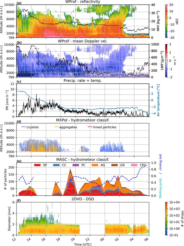
418                     J. Gehring et al.: Precipitation measurements during the ICE-POP 2018 campaign in South Korea

1   Introduction                                                 the energy and hydrological budgets of the Greenland Ice
                                                                 Sheet. In Antarctica, the APRES3 (Antarctic Precipitation,
Precipitation measurements in mountainous regions are            Remote Sensing from Surface and Space) field campaign
paramount to characterise the spatial distribution of pre-       (Genthon et al., 2018) provided the first dual-polarisation
cipitation and understand the effect of orography on mi-         radar measurements from November 2015 to February 2016.
crophysics. South Korea’s geographical environment pro-          Along with snowflake photographs, measurements of micro
vides a unique setting for precipitation studies: its location   rain radar and lidar, the dataset led to unprecedented insights
on a mountainous peninsula in the mid-latitudes is prone         into Antarctic snowfall microphysics (Grazioli et al., 2017a).
to large moisture advection by baroclinic systems and oro-       Finally, the AWARE (U.S. Department of Energy Atmo-
graphic lifting driving cloud and precipitation formation.       spheric Radiation Measurement (ARM) West Antarctic Ra-
Unlike other mountain ranges such as the Alps, the Rock-         diation Experiment) campaign (Lubin et al., 2020) gathered
ies, the Olympic Mountains, the Cascade Mountains and            cloud radars, lidars, radiometers, aerosols and microphysi-
the Coast Mountains (Bougeault et al., 2001; Saleeby et al.,     cal measurements from December 2015 to December 2016
2009; Houze et al., 2017; Stoelinga et al., 2003; Joe et al.,    at McMurdo Station, Antarctica. This unique dataset offers
2010), the study of precipitation in the Taebaek Mountains       numerous cases for mixed-phase cloud parameterisation in
across the Korean Peninsula has not been as extensive. Kim       weather and climate models. The measurements of these field
et al. (2018) investigated the microphysics of two snowfall      campaigns allowed for innovative studies and new insights
events in the Taebaek Mountains during the Experiment on         into cloud and precipitation processes in these various re-
Snow Storms At Yeongdong (ESSAY) campaign using ra-              gions (Kalesse et al., 2016; von Lerber et al., 2017; Grazi-
diosoundings, snowflake images and numerical simulations.        oli et al., 2017b; Cole et al., 2017; Zagrodnik et al., 2019).
They suggested that future field campaigns should include        For a better understanding of cloud and precipitation pro-
dual-polarisation radars and a multi-angle snowflake camera      cesses in the Taebaek Mountains, a field campaign combin-
(MASC) to better understand the microphysics of precipita-       ing remote sensing and in situ measurements is needed. The
tion in this region. There was hence a need for a precipita-     PyeongChang 2018 Olympic and Paralympic winter games
tion measurement campaign in the Taebaek Mountains with          were the opportunity to initiate interest and collaboration for
remote sensing and in situ measurements.                         such a campaign. Indeed, accurate weather forecasts during
   Several past field campaigns demonstrated the useful-         Winter Olympic Games are an organisational need and a real
ness of combined remote sensing and in situ measurements         scientific challenge. It is also a great opportunity to foster
for snowfall studies. The TOSCA (Technology Options and          international collaboration and gather the atmospheric sci-
Strategies towards Climate friendly transport) project in the    ence community. One successful example of such a joint ef-
Bavarian Alps in Germany (Löhnert et al., 2011) com-             fort was the Science of Nowcasting Olympic Weather for
bined vertically pointing radars, radiometers and optical dis-   Vancouver 2010 campaign, which led to novel findings on
drometers among others to better characterise the vertical       precipitation (Thériault et al., 2012; Schuur et al., 2014;
distribution of snowfall for satellite retrievals and numeri-    Berg et al., 2017) and nowcasting (Haiden et al., 2014), as
cal model validations. During the 2015/16 fall–winter sea-       well as to new instrumental developments (Boudala et al.,
son, the OLYMPEX (Olympic Mountain Experiment) cam-              2014). Along the same line, the Korea Meteorological Ad-
paign (Houze et al., 2017) took place in the vicinity of the     ministration organised the International Collaborative Ex-
mountainous Olympic Peninsula, USA, to study how Pa-             periments for PyeongChang 2018 Olympic and Paralympic
cific precipitation systems are influenced by the orography.     winter games (ICE-POP 2018). The main goals of ICE-POP
The BAECC (Biogenic Aerosols–Effects on Clouds and Cli-          2018 were to support forecasters with high-resolution model
mate) field campaign (Petäjä et al., 2016) provided 8 months     simulations and radar data, as well as to gain more insight
of measurements in Hyytiälä, Finland, to study biogenic          into orographic precipitation in the Taebaek Mountains. For
aerosols, clouds and precipitation and their interactions.       this purpose, remote sensing and in situ measurements of
In situ and remote sensing instruments have also proven very     clouds and precipitation were conducted in the province of
useful to study atmospheric radiation, cloud and precipita-      Gangwon-do between November 2017 and May 2018.
tion properties in polar regions. The North Slope of Alaska         This article presents the data collected by the Envi-
atmospheric observatory (Verlinde et al., 2016) in Utqiaġvik    ronmental Remote Sensing Laboratory of the École Poly-
(formerly Barrow) and Oliktok provides a long series of mea-     technique Fédérale de Lausanne during ICE-POP 2018. It
surements including radiometers, lidars, cloud radars and a      includes measurements from an X-band dual-polarisation
MASC among many other instruments. Another major Arc-            Doppler radar, a W-band Doppler cloud profiler, a multi-
tic measurement site is located at Summit Camp, Greenland,       angle snowflake camera and a two-dimensional video dis-
where the ICECAPS (Integrated Characterization of Energy,        drometer. Such a dataset is unique, as it includes multi-
Clouds, Atmospheric State, and Precipitation at Summit;          frequency radar and ground-based measurements in a region
Shupe et al., 2013) field campaign was conducted to collect      where similar measurements were scarce before ICE-POP
measurements of radiation, clouds and precipitation to study     2018. As shown in Gehring et al. (2020b) it is a useful dataset

Earth Syst. Sci. Data, 13, 417–433, 2021                                          https://doi.org/10.5194/essd-13-417-2021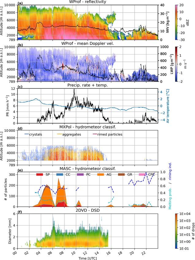
J. Gehring et al.: Precipitation measurements during the ICE-POP 2018 campaign in South Korea 419
for snowfall microphysics studies and could also be relevant at 90◦ elevation in FFT mode was performed for differential
for validation of numerical weather prediction models. Sec- reflectivity calibration.
tion 2 presents the campaign and the instrumental setup, and
Sect. 3 describes the data processing. Section 4 illustrates the 2.2 W-band cloud profiler: WProf
dataset with measurements and hydrometeor classifications
corresponding to the four events with the largest accumula- A W-band Doppler cloud profiler (WProf) was deployed at
tion. Section 6 closes this paper with concluding remarks. the Mayhills site (MHS). WProf is a frequency-modulated
continuous-wave (FMCW) radar operating at 94 GHz at a
2 Measurement sites and instruments single polarisation. It allows for measuring with different
ranges and Doppler resolutions, typically using three vertical
In this study, we will focus on the data collected by a mo- chirps (Table 1). The main variables retrieved are the equiva-
bile X-band dual-polarisation Doppler (polarimetric) radar lent reflectivity factor Z, the mean Doppler velocity VD , the
(MXPol), a W-band Doppler cloud profiler (WProf), a multi- Doppler spectral width σv (m s−1 ), skewness and kurtosis.
angle snowflake camera (MASC) and a two-dimensional The full Doppler spectrum is also available. More details on
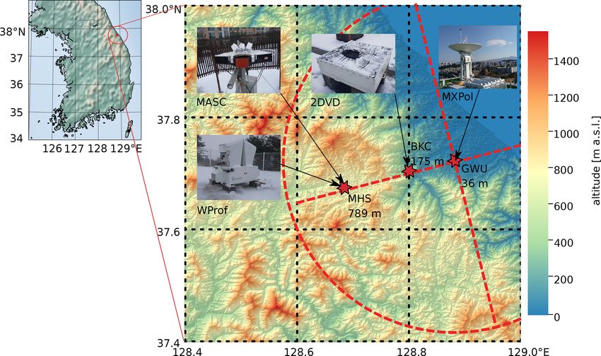
video disdrometer (2DVD). Figure 1 shows the location of WProf can be found in Küchler et al. (2017). WProf contains
the instruments. The first measurement site was located at an 89 GHz radiometer, which can be used to retrieve the liq-
Gangneung–Wonju National University (GWU) at 66 m a.s.l. uid water path (LWP) and the integrated water vapour (IWV).
The second measurement site was at the Bokwang 1-ri We computed LWP and IWV using the method described in
community centre (BKC), 6 km inland from Gangneung at Billault-Roux and Berne (2020). The brightness temperature
175 m a.s.l. The third measurement site, Mayhills (MHS), measurements had a bias of 20 K, which we corrected. Af-
was located in the county of Pyeongchang at 789 m a.s.l., ter correction the root mean squared error (RMSE) is 2.88 K.
19 km inland of GWU. Radiosoundings were launched by The RMSE of LWP and IWV are 86.5 and 1.72 kg m2 , re-
the Korea Meteorological Administration (KMA) in Daeg- spectively, taking radiosoundings as the reference. More in-
wallyeong (DGW), 2 km from MHS. formation on the uncertainty of this algorithm can be found
in Billault-Roux and Berne (2020). In particular, note that
the accuracy is deteriorated in case of intense precipita-
2.1 X-band polarimetric radar: MXPol
tion. WProf was calibrated by the manufacturer, Radiometer
The scanning X-band polarimetric radar, named MXPol, was Physics GmbH (RPG), just before the ICE-POP 2018 cam-
installed in GWU on the coast of the East Sea (Sea of Japan). paign. This included a calibration of the 89 GHz radiometer
The main variables retrieved from MXPol measurements with liquid nitrogen and a calibration of the radar with dis-
in dual-pulse pair (DPP) mode are the equivalent reflectiv- drometers following the method of Myagkov et al. (2020).
ity factor at horizontal polarisation ZH (dBZ), the differ- The uncertainty of WProf reflectivity calibration is ±1 dB.
ential reflectivity ZDR (dB), the specific differential phase Note that compared to Gehring et al. (2020b) the calibra-
shift on propagation Kdp (◦ km−1 ), the copolar correlation tion was updated following RPG’s recommendations, and
coefficient ρhv , the mean Doppler velocity VD (m s−1 ) and hence the Ze values of WProf do not match with those of
the Doppler spectral width σv (m s−1 ). Additionally, in fast this article. This calibration correction was applied on the
Fourier transform (FFT) mode, the full Doppler spectrum at data available in Gehring et al. (2020a). The radomes were
0.17 m s−1 resolution is retrieved at each range gate. MXPol in good shape and were not changed between the calibra-
operates at 9.41 GHz with a typical angular resolution of 1◦ , tion and the field campaign. The blowers, which prevent liq-
range resolution of 75 m, non-ambiguous range of 120 km, uid water from accumulating on the radomes, were switched
and Nyquist velocity of 39 m s−1 in DPP or 11 m s−1 in FFT on all the time. The radar pointing was evaluated by check-
mode. Only the data up to the 28 km range are saved, since ing the levels at the beginning and the end of the campaign.
the decrease in sensitivity and increase in sampling volume The levels showed that the radar was pointing almost per-
make the further gates less relevant for microphysical stud- fectly vertically. However, since the vertical alignment was
ies. A more technical description of MXPol can be found in not monitored constantly, the spectral and Doppler veloc-
Schneebeli et al. (2013). The main scan cycle was composed ity data should be interpreted carefully, especially in case of
of two hemispherical range height indicators (RHIs) at 227 strong horizontal winds.
and 317◦ azimuth in FFT and DPP modes, respectively. The
former is towards MHS, while the latter is perpendicular to 2.3 Multi-angle snowflake camera: MASC
this direction following the coast as shown by the red dot-
ted line in Fig. 1. The two RHIs were followed by one plan A multi-angle snowflake camera (MASC) was deployed in a
position indicator (PPI) in DPP mode at 6◦ elevation. The double-fence windshield in MHS. The MASC is composed
cycle was either completed by two other RHIs or PPIs de- of three coplanar cameras separated by an angle of 36◦ .
pending on the event. The scan cycle had a 5 min duration As hydrometeors fall in the triggering area, high-resolution
and was repeated indefinitely. At least once an hour, a PPI stereographic pictures are taken, and their fall velocities are
https://doi.org/10.5194/essd-13-417-2021 Earth Syst. Sci. Data, 13, 417–433, 2021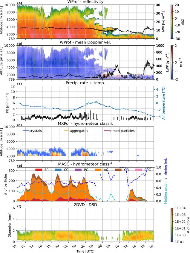
420                       J. Gehring et al.: Precipitation measurements during the ICE-POP 2018 campaign in South Korea

Figure 1. Location of the instruments used for this dataset. A digital elevation model shows the topography of the region and its location
within South Korea. The red dotted lines and circle show the extent of the main RHIs (27.2 km) and PPIs (28.4 km radius), respectively. Note
that the MASC was located at BKC from 15 November 2017 to 20 February 2018 and at MHS afterwards. Adapted from Gehring et al.
(2020b).

Table 1. Description of WProf chirps.

                        Range              Range resolution    Doppler interval        Doppler resolution    Integration time
              chirp2    [2016, 9984] m     32.5 m              [−5.1, 5.1] m s−1       0.020 m s−1           0.82 s
              chirp1    [603, 1990] m      11.2 m              [−5.1, 5.1] m s−1       0.020 m s−1           0.37 s
              chirp0    [100, 598] m       5.6 m               [−7.16, 7.13] m s−1     0.028 m s−1           0.18 s

measured. A complete description of the MASC can be found               dimensional profiles are then combined to form a two-
in Garrett et al. (2012). The MASC images were used as                  dimensional view of the particle. Horizontal wind induces a
input parameters to a solid hydrometeor classification algo-            horizontal displacement of the particles such that the super-
rithm. Individual particles are classified into six solid hy-           position of the one-dimensional sections can lead to distorted
drometeor types, namely small particles (SPs), columnar                 particles. This issue is thoroughly investigated with numeri-
crystals (CCs), planar crystals (PCs), a combination of col-            cal simulations in Nešpor et al. (2000). The two orthogonal
umn and plate crystals (CPCs), aggregates (AGs), and grau-              two-dimensional projections yield three-dimensional shape
pel (GR). In addition a riming index ranging from 0 to 1 is             information, which can be used to compute the equivalent
computed. A detailed explanation of the algorithm is pro-               drop diameter and the aspect ratio. This makes it possible
vided in Praz et al. (2017). Note that the riming index of              to compute the raindrop size distribution (DSD). Since the
melting particles and raindrops computed by this method is              vertical distance between the two light sheets is known, the
usually quite high. One should not consider the riming index            particles’ fall velocities can also be computed. 2DVD data
for particles with a melting probability higher than 50 %.              can also be used for snowfall microphysics studies. Brandes
                                                                        et al. (2007) derived the particle size distribution (PSD) from
                                                                        2DVD data in Colorado. Huang et al. (2010) and Huang et al.
2.4   Two-dimensional video disdrometer: 2DVD                           (2015) used a 2DVD to derive radar reflectivity–snowfall rate
                                                                        relations. Finally Grazioli et al. (2014) used 2DVD data to
A two-dimensional video disdrometer (2DVD) was deployed                 develop a supervised hydrometeor classification method.
in BKC. A detailed description of the instrument can be
found in Kruger and Krajewski (2002) and Schönhuber et al.
(2007). Here we will describe the general measurement prin-
ciple. Two orthogonal light sources are projected onto a line-
scan camera. Particles falling through the light sheets project
a one-dimensional section on the photodetectors. These one-

Earth Syst. Sci. Data, 13, 417–433, 2021                                                   https://doi.org/10.5194/essd-13-417-2021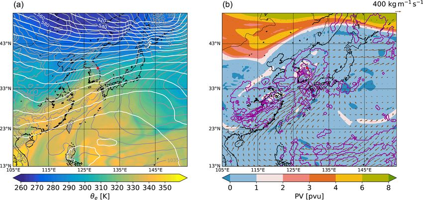
J. Gehring et al.: Precipitation measurements during the ICE-POP 2018 campaign in South Korea                                          421

Figure 2. Distribution of two-way attenuation (up to 10 km) at 94 GHz for dry air (a), water vapour (b) and total attenuation (c) computed
with PAMTRA (Passive and Active Microwave TRansfer Model) for all profiles of WProf interpolating at 5 min the radiosounding data.

Figure 3. Range distribution of reflectivity values for (a) WProf and (b) MXPol during all precipitation events (see Fig. 4). The colour bar
shows the number of measurements per range gate. The total number of measurement points is 1.24 × 10⁸ for WProf and 2.25 × 10⁸ for
MXPol.

Table 2. Specifications of MXPol and WProf.                             Table 3. Data amount for all instruments.

       Specifications        MXPol               WProf                                  MXPol     62 h, 4166 RHIs, 2036 PPIs
                                                                                        WProf     121 h, 146 548 profiles
       Frequency             9.41 GHz            94 GHz                                 MASC      29 886 triplets
       3 dB beamwidth        1.27◦               0.53◦                                  2DVD      2 304 730 drops
       Sensitivity at 8 km   5 dBZ               −40 dBZ
       Transmission type     Pulsed              FMCW
       Polarisation          Dual polarisation   Single polarisation
       Range resolution      75 m                5.6, 11.2, 32.5 m      3.1.1    Calibration
                                                                        To monitor the stability of the radar signal, a radar tar-
                                                                        get simulator (RTS, http://www.palindrome-rs.ch/products/
3     Data processing
                                                                        radar-target-simulator/, last access: 4 September 2020) de-
3.1    MXPol                                                            veloped by Palindrome Remote Sensing GmbH was installed
                                                                        during the campaign. Unfortunately, due to technical issues
First, the noise floor is determined from the raw power fol-            during the campaign, the data could not be used for calibra-
lowing the method from Hildebrand and Sekhon (1974).                    tion of the radar. However, we conducted dedicated calibra-
Then, the polarimetric variables are computed based on the              tion measurements with the RTS in July 2018 just after the
backscattering covariance matrix following Doviak and Zr-               ICE-POP 2018 campaign. The results showed that the reflec-
nic (1993). The computation of Kdp is based on an ensemble              tivity measurements have errors smaller than 1 dBZ.
of Kalman filters as detailed in Schneebeli et al. (2014).

https://doi.org/10.5194/essd-13-417-2021                                                    Earth Syst. Sci. Data, 13, 417–433, 2021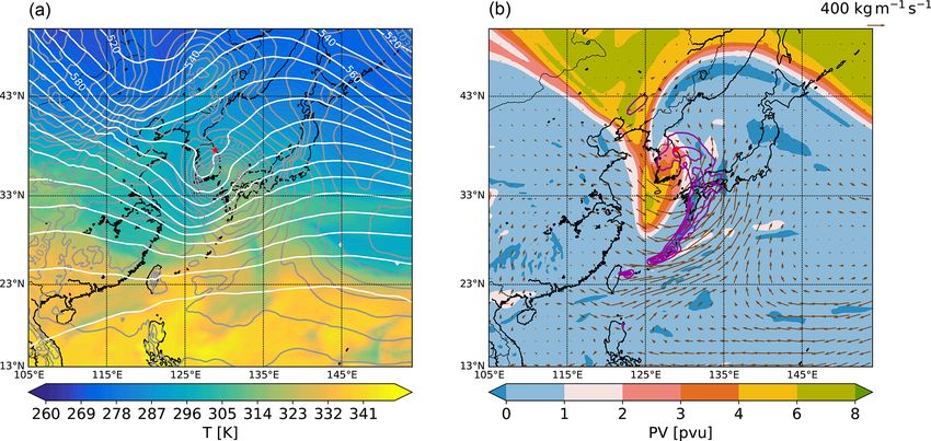
422                     J. Gehring et al.: Precipitation measurements during the ICE-POP 2018 campaign in South Korea

3.1.2   Hydrometeor classification                                 Table 4. Date and time of the start and end of the precipitation
                                                                   events. The four major events presented here are highlighted in bold.
The dual-polarisation observables were used to feed the hy-
drometeor classification from Besic et al. (2016). The cen-                     ID   Start (UTC)          End (UTC)
troids of all four polarimetric variables used for the classi-                  1    06:30 25 Nov 2017    17:30
fication have been trained on MXPol data from various field                     2    00:00 24 Dec 2017    07:00
campaigns in the Swiss Alps, in Ardèche (France), in Antarc-                    3    00:00 9 Jan 2018     18:00
                                                                                4    20:00 16 Jan 2018    23:59
tica and on the present dataset in South Korea. Recently,
                                                                                5    06:30 22 Jan 2018    14:30
Besic et al. (2018) developed a de-mixing approach of this                      6    00:00 28 Feb 2018    23:59
hydrometeor classification, in which the proportion of hy-                      7    12:00 4 Mar 2018     06:00 5 Mar 2018
drometeors for each radar sampling volume is estimated, in-                     8    10:00 7 Mar 2018     18:00 8 Mar 2018
stead of one dominant class. The classes are crystals, aggre-
gates, light rain, rain, rimed ice particles, vertically aligned
ice, wet snow, ice hail, and high-density graupel and melt-        the values within 0.32 dB. This median value of 2.66 dB was
ing hail. This approach is essentially built upon the concept      subtracted from all ZDR measurements to get the corrected
of entropy, as defined in Besic et al. (2016), which reflects      ZDR dataset.
the uncertainty with which a hydrometeor class is assigned
to one sampling volume. This de-mixing method has the ad-
vantage of revealing the spectrum of hydrometeors present in
the observed precipitation. The classification was applied to
all RHIs of the precipitation events shown in Fig. 4. Only the
data above 2000 m a.s.l. have been selected for the hydrom-
eteor classification shown in Sect. 4 because of ground echo
contamination and partial beam filling below this altitude.

3.1.3   Differential reflectivity bias correction

For a correct interpretation of ZDR , the offset introduced by
the existence of differences in amplitude in the horizontal
and vertical channels needs to be subtracted. This calibra-
tion can be achieved by analysing ZDR values in a specific
subset of the range gates of the vertical PPI, which were per-
formed at least once an hour during the whole campaign. Un-        Figure 4. Precipitation accumulation (blue bars), mean precipita-
fortunately, MXPol is affected by extremely high ZDR values        tion rates (red star) in mm h−1 , maximum temperature (red cross),
                                                                   mean temperature (black cross) and minimum temperature (blue
in the low gates, probably caused by issues on the transmit-
                                                                   cross). The black line shows the mean precipitation rate during pre-
receive limiter. Therefore, a classical calibration procedure      cipitation events. The duration of the events is written on top of the
such as the one described in Gorgucci et al. (1999) cannot be      bars. The precipitation and temperature data come from a Pluvio2
applied. Instead, we decided to select the range interval used     weighing rain gauge and a Vaisala weather station located in MHS.
for the correction among the upper gates, which were unaf-         The Pluvio2 data are not part of this dataset but can be requested
fected by the issue. The first step of the calibration procedure   from the corresponding author.
was the removal of data with signal-to-noise ratios lower than
5 dB or ρhv < 0.95. For each PPI, we also removed the range
gates in which we encountered at least one non-valid ZDR
                                                                   3.2   MASC
measurement to avoid introducing a bias caused by some an-
gles being overrepresented. Subsequently, we computed, for         The raw data from the MASC are stereographic photographs
each range gate, the standard deviation of the ZDR distribu-       of hydrometeors and measurements of fall velocities. Praz
tion over the whole campaign duration. This standard devia-        et al. (2017) developed a hydrometeor classification and rim-
tion is remarkably constant more than 1 km above the radar,        ing index estimation of MASC pictures based on a multi-
while its magnitude increases rapidly in the closest gates, due    nomial logistic regression model. More recently, Hicks and
to the issue mentioned before. After computing the median          Notaroš (2019) used convolutional neural networks to clas-
of these values in the top 25 % of the range gates, we im-         sify MASC snowflake images. In this paper, we will use the
pose a maximum threshold of 0.1 dB on the absolute differ-         algorithm from Praz et al. (2017) to classify the MASC data
ence between the standard deviation at each range gate and         collected during ICE-POP 2018. We will show the hydrom-
the median value. The median of all ZDR values from the            eteor classification, as well as the riming index and melting
range gates satisfying the condition is 2.66 dB with 50 % of       probability results. Note that the riming index of small par-

Earth Syst. Sci. Data, 13, 417–433, 2021                                              https://doi.org/10.5194/essd-13-417-2021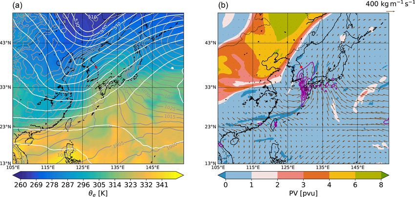
J. Gehring et al.: Precipitation measurements during the ICE-POP 2018 campaign in South Korea                                             423

Figure 5. Synoptic meteorological fields at 12:00 UTC on 25 November 2017 from the ERA5 reanalysis. (a) Sea-level pressure (grey
contours, labels in hPa), 500 hPa geopotential height (white contours, labels in decametres) and 850 hPa equivalent potential temperature
(θe colours). (b) Potential vorticity at 315 K (colours; potential vorticity unit (PVU) = 1 × 10⁻⁶ K m2 kg−1 s−1 ), vertically integrated water
vapour flux (brown arrows) and precipitation rate (purple contours every 2 mm h−1 ).

ticles is not reliable, since it is computed over a few pixels            determined using the method from Hildebrand and Sekhon
only. Therefore we discard small particle in the time series              (1974). The moments (VD , Z, σv , skewness and kurtosis) are
of riming index (i.e. Figs. 6, 8, 10, 12). In addition, raindrops         then computed from the de-aliased spectra above the noise
appear as small bright spots in MASC images (reflection of                floor.
flashes) and are hence classified as small particles. There-
fore, removing small particles from the riming index statis-
tics avoids the bias related to raindrops.                                3.3.1    Atmospheric gas attenuation
   Schaer et al. (2020) developed a method to classify MASC
                                                                          To correct for attenuation due to atmospheric gases, we used
images as blowing snow, precipitation or a mixture of those.
                                                                          the Passive and Active Microwave TRansfer Model (PAM-
This makes it possible to filter the results and minimise the
                                                                          TRA, Mech et al., 2020) available at https://github.com/
influence of possible blowing snow. Even though a double-
                                                                          igmk/pamtra (last access: 27 May 2020) and humidity, tem-
fence windshield was present during the ICE-POP 2018 cam-
                                                                          perature and pressure profiles from radiosoundings launched
paign, 31 % of the particles were classified either as a mixture
                                                                          at DGW. Radiosoundings were usually available every 3 h
of precipitation and blowing snow or pure blowing snow. In
                                                                          but sometimes up to 12 h. In order to quantify the tempo-
the present dataset, all particles are retained, but the informa-
                                                                          ral variability, we computed the variogram of IWV from all
tion needed to filter out blowing snow particles is added. As
                                                                          radiosoundings and concluded that the decorrelation time is
explained in Schaer et al. (2020) a threshold of 0.193 on the
                                                                          long enough, so we can expect relatively accurate interpo-
normalised angle ψ can be used with ψ < 0.193 correspond-
                                                                          lated values in between radiosoundings. We hence decided
ing to pure precipitation. The results of the hydrometeor clas-
                                                                          to compute a linear interpolation between the two nearest ra-
sification shown in Sect. 4 correspond to pure precipitation
                                                                          diosoundings in time to get the profiles at a 5 min resolution,
only.
                                                                          which was then used to compute the gas attenuation and ap-
                                                                          plied to each WProf profile. Figure 2 shows the histograms
3.3   WProf                                                               of dry air, water vapour and total two-way attenuation at the
                                                                          W-band from 30 November 2017 to 31 March 2018, which
The raw data from WProf were saved without any filtering,                 corresponds to the period during which radiosoundings are
in the form of raw Doppler spectra. The spectra are then de-              available. Outside of this period, the WProf reflectivity mea-
aliased with an algorithm based on the minimisation of the                surements were not corrected for attenuation. For dry air the
spectral width at each range gate, similar to Ray and Ziegler             values range from about 0.26 to 0.33 dB. For water vapour,
(1977). This method assumes aliasing up to one folding,                   the values range from nearly 0 to 1.75 dB. The attenuation
which is sufficient for the Nyquist intervals considered here             depends on the absolute humidity, and hence the range of
(Table 1). From the de-aliased spectra, the noise floor was               values is larger, going from a very dry air to a saturated envi-

https://doi.org/10.5194/essd-13-417-2021                                                      Earth Syst. Sci. Data, 13, 417–433, 2021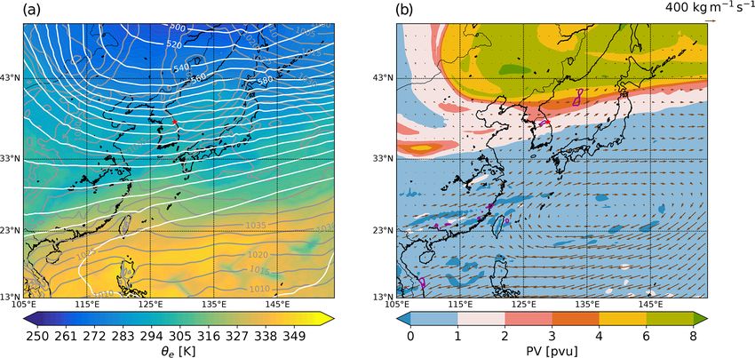
424                       J. Gehring et al.: Precipitation measurements during the ICE-POP 2018 campaign in South Korea

Figure 6. Time series on 25 November 2017 of (a) reflectivity and IWV, (b) mean Doppler velocity (vel.) (defined positive upwards) and
LWP from WProf, (c) precipitation rate (PR) and air temperature at MHS, and (d) hydrometeor classification (classif.) based on MXPol
RHIs towards MHS (averaged between 7 and 20 km). Only data with an elevation angle between 5 and 45◦ are considered. The isolines
represent the proportion of each hydrometeor class normalised by the average number of pixels per time step. The contour interval is 2 %.
The blue contours represent crystals; the yellow ones represent aggregates; and the red ones represent rimed particles. The results are shown
only above 2000 m, since the lower altitudes are contaminated by ground echoes. (e) Hydrometeor classification from the MASC, melting
probability (prob.) and riming index (ind.) (see Sects. 2.3 and 3.2 for a description) and (f) drop size distribution from the 2DVD. For this
event, the MASC was located at BKC at 175 m. a.s.l. together with the 2DVD. The gap around 16:00 UTC of precipitation rate in (c) is due
to a technical issue with the rain gauge.

ronment. The total two-way attenuation (up to 10 km) varies              3.4   Sensitivity
between 0.3 to 2 dB.
                                                                         To visualise the sensitivity of WProf and MXPol, Fig. 3
                                                                         shows the empirical joint distributions of range and reflec-
                                                                         tivity values during all precipitation events of the ICE-POP
                                                                         2018 campaign. The minimum measured reflectivity values

Earth Syst. Sci. Data, 13, 417–433, 2021                                                     https://doi.org/10.5194/essd-13-417-2021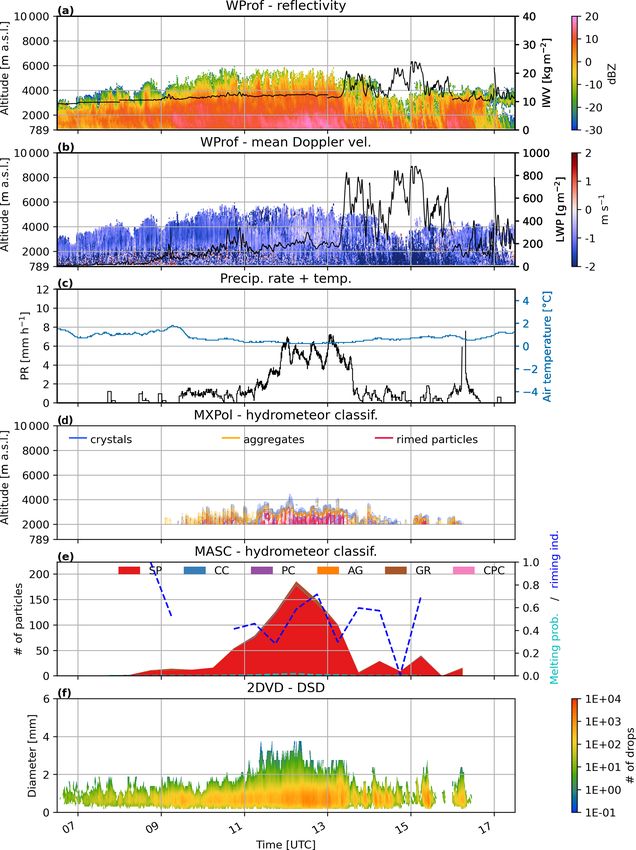
J. Gehring et al.: Precipitation measurements during the ICE-POP 2018 campaign in South Korea                                            425

Figure 7. Synoptic meteorological fields at 12:00 UTC on 28 February 2018 from the ERA5 reanalysis. (a) Sea-level pressure (grey contours,
labels in hPa), 500 hPa geopotential height (white contours, labels in dam) and 850 hPa equivalent potential temperature (θe colours). (b)
Potential vorticity at 315 K (colours; potential vorticity unit (PVU) = 1×10⁻⁶ K m2 kg−1 s−1 ), vertically integrated water vapour flux (brown
arrows) and precipitation rate (purple contours every 2 mm h−1 ).

represent the sensitivity. A threshold on the signal-to-noise            measurement duration from MXPol is about half that from
ratio of 0 dB was applied on MXPol and WProf data in all                 WProf, which measured continuously. The number of triplets
figures presented. For WProf (Fig. 3a) we can clearly see the            captured by the MASC indicates the number of sets of three
effect of the three vertical chirps on the minimum detectable            pictures captured by the three cameras. For each picture, the
reflectivity. One can see that WProf has a higher sensitivity            classification selects one particle that is in focus. The max-
than MXPol at all range gates.                                           imum rate of images is 2 Hz; hence only two hydrometeors
                                                                         can be identified every second. The 2DVD measures continu-
                                                                         ously at a rate of 34.1 kHz and can identify multiple particles
4   Precipitation events                                                 in its sampling area, unlike the MASC. This explains why
                                                                         the number of particles captured by the 2DVD is 2 orders of
Figure 4 shows precipitation and temperature information
                                                                         magnitude greater than the number of triplets of the MASC.
during the precipitation events. Table 4 shows the exact date
and time of the different events. The atmospheric condi-
tions during the ICE-POP 2018 campaign were climatolog-                  4.1    25 November 2017
ically cold and dry. The winter of 2018 (December 2017–
February 2018) had a total precipitation accumulation of                 The 25 November 2017 event has the third-largest precipita-
93 mm in MHS, while the climatological value (KMA, 2011)                 tion accumulation but the second-largest mean precipitation
is 153 mm in Daegwallyeong, 2 km from MHS. The major                     rate (see Fig. 4). Figure 5 shows a strong westerly flow as-
precipitation event on 28 February 2018 contributed to 62 %              sociated with a broad upper-level trough. Analysis of back-
of the precipitation accumulation during winter 2018, which              ward trajectories (not shown) revealed that the moisture was
shows that the rest of the winter was extremely dry (36 mm               pumped from the Yellow Sea and lifted over the topography
excluding the 28 February event). March featured a few sig-              leading to a broad cloud and precipitation system.
nificant precipitation events, leading to 83 mm of precipita-               Figure 6a shows the reflectivity measured by WProf. The
tion accumulation, while the climatological value is 76 mm.              precipitating cloud is shallow with a cloud top at 4800 m.
We have four main events, which we will present in this sec-             Precipitation starts at 08:00 UTC and lasts until 16:00 UTC.
tion: 25 November 2017, 28 February 2018, and 4 and 7                    Figure 6b shows the Doppler velocity measured by WProf.
March 2018. These events stand out due to their significant              Negative (positive) values represent a relative displacement
precipitation accumulation. Table 3 shows the amount of data             towards (away from) the radar. Except for some local tur-
collected by each instrument. The measurement time from                  bulence below 2000 m, there are no significant updraughts
MXPol does not take into account the repositioning of the an-            in the cloud. Note that the precipitation rate data shown in
tenna between each scan, which typically takes the same time             Fig. 6c are not part of the presented dataset but can be re-
as the scan averaged over the whole cycle. This is why the               quested from the corresponding author. One can observe that

https://doi.org/10.5194/essd-13-417-2021                                                     Earth Syst. Sci. Data, 13, 417–433, 2021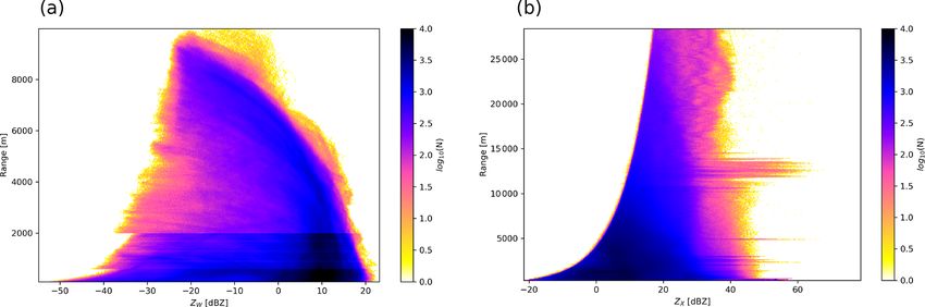
426                       J. Gehring et al.: Precipitation measurements during the ICE-POP 2018 campaign in South Korea

Figure 8. Time series on 28 February 2018 of (a) reflectivity and IWV, (b) mean Doppler velocity (vel.) (defined positive upwards) and
LWP from WProf, (c) precipitation rate (PR) and air temperature at MHS, and (d) hydrometeor classification (classif.) based on MXPol
RHIs towards MHS (averaged between 7 and 20 km). Only data with an elevation angle between 5 and 45◦ are considered. The isolines
represent the proportion of each hydrometeor class normalised by the average number of pixels per time step. The contour interval is 2 %.
The blue contours represent crystals; the yellow ones represent aggregates; and the red ones represent rimed particles. The results are shown
only above 2000 m, since the lower altitudes are contaminated by ground echoes. (e) Hydrometeor classification from the MASC, melting
probability (prob.) and riming index (ind.) (see Sects. 2.3 and 3.2) and (f) drop size distribution from the 2DVD. Note that the MASC was
located at MHS at 789 m a.s.l. as WProf, while the 2DVD was located at BKC at 175 m a.s.l.

rimed particles dominate below 3000 m a.s.l. from 11:30 to               ure 6f shows the DSD computed from 2DVD data at BKC.
13:30 UTC (dominance of red shades in Fig. 6d).                          The largest raindrops are observed during the most intense
   Figure 6e shows a time series of the classification from              precipitation period (11:00–13:00 UTC) and correspond to
the MASC. At this time, the MASC was in BKC at only                      the highest vertical extension of the cloud.
175 m a.s.l., and it observed almost exclusively raindrops,
which are classified as small particles (Praz et al., 2017). Fig-

Earth Syst. Sci. Data, 13, 417–433, 2021                                                    https://doi.org/10.5194/essd-13-417-2021
J. Gehring et al.: Precipitation measurements during the ICE-POP 2018 campaign in South Korea                                            427

Figure 9. Synoptic meteorological fields at 15:00 UTC on 4 March 2018 from the ERA5 reanalysis. (a) Sea-level pressure (grey contours,
labels in hPa), 500 hPa geopotential height (white contours, labels in dam) and 850 hPa equivalent potential temperature (θe colours). (b)
Potential vorticity at 315 K (colours; potential vorticity unit (PVU) = 1×10⁻⁶ K m2 kg−1 s−1 ), vertically integrated water vapour flux (brown
arrows) and precipitation rate (purple contours every 2 mm h−1 ).

4.2   28 February 2018                                                   tation rates around 06:00 and 10:00 UTC (Fig. 8c) correlate
                                                                         well with regions of high reflectivity extending up to about
The 28 February 2018 event stands out as the most intense of
                                                                         4000 m a.s.l. During the passage of the front aggregates pre-
the whole campaign, in terms of accumulation and mean pre-
                                                                         vail, while from 06:00 to 08:00 UTC rimed particles domi-
cipitation rate. At 00:00 UTC (not shown) a prominent po-
                                                                         nate (Fig. 8d).
tential vorticity (PV) streamer over eastern China and a low-
                                                                            Figure 8e shows the time series of the MASC classifica-
pressure system eastward over the Yellow Sea are present.
                                                                         tion. There are periods of missing data because the cameras
The PV streamer intensifies the surface cyclone, and by
                                                                         were covered with rime. The event was dominated by aggre-
12:00 UTC on 28 February (Fig. 7) the system is fully de-
                                                                         gates, except at the end, where the temperature was colder
veloped with the warm front passing over Pyeongchang and
                                                                         and graupel and small particles are present. Note that the
leading to the observed precipitation. Note that the cyclone
                                                                         classification of Praz et al. (2017) classifies only fully rimed
intensified by 25 hPa between 18:00 UTC on 27 February and
                                                                         particles as graupel. The class aggregates also contain rimed
12:00 UTC on 28 February due to the upper-level forcing
                                                                         particles, which explains why the period dominated by rimed
from the PV streamer. This event is presented in more de-
                                                                         particles in Fig. 8d (06:00 to 08:00 UTC) is not visible in the
tails in Gehring et al. (2020b).
                                                                         MASC classification as graupel particles. However, it is clear
   At 00:00 UTC on 28 February, the nimbostratus (i.e. pre-
                                                                         from the riming index that rimed particles are present during
cipitating cloud associated with the warm front) can be ob-
                                                                         this period.
served above 2000 m, while fog is forming below 1000 m
(Fig. 8a). Between the fog and the nimbostratus base, a dry
layer is present where the precipitation from the nimbostra-             4.3    4 March 2018
tus sublimates to form virgas. At 03:00 UTC precipitation
reaches the ground and lasts until 16:00 UTC. As tempera-                The 4 March 2018 event has the second-largest precipitation
tures at MHS are between 0 and 2 ◦ C before 06:00 UTC, the               accumulation. Figure 9 shows the synoptic conditions. There
liquid water attenuation of the melting snowflakes can lead              is a strong south-westerly flow advecting significant mois-
to underestimation of the reflectivity measurements of both              ture from the Yellow Sea, as can be seen by the integrated
MXPol and WProf. After 06:00 UTC, the temperatures at                    vapour fluxes (brown arrows) reaching 1000 kg m−1 s−1 and
MHS are below freezing (Fig. 8c), and hence there is almost              a low-pressure system located south of the Korean Penin-
no liquid water attenuation (attenuation from supercooled                sula. This large moisture transport leads to widespread pre-
liquid water, SLW, droplets can be neglected). One can no-               cipitation over the Korean Peninsula with a maximum over
tice a region of embedded convection between 07:30 and                   the centre of South Korea. The equivalent potential tempera-
08:00 UTC and turbulence around 4000 m between 08:00                     ture shows the presence of warm and humid air reaching the
and 10:00 UTC (Fig. 8b). The two first maxima of precipi-                cyclone’s centre. The large sea-level pressure gradient on the

https://doi.org/10.5194/essd-13-417-2021                                                     Earth Syst. Sci. Data, 13, 417–433, 2021
428 J. Gehring et al.: Precipitation measurements during the ICE-POP 2018 campaign in South Korea
Figure 10. Time series from 4 to 5 March 2018 of (a) reflectivity and IWV, (b) mean Doppler velocity (vel.) (defined positive upwards)
and LWP from WProf, (c) precipitation rate (PR) and air temperature at MHS, and (d) hydrometeor classification (classif.) based on MXPol
RHIs towards MHS (averaged between 7 and 20 km). Only data with an elevation angle between 5 and 45◦ are considered. The isolines
represent the proportion of each hydrometeor class normalised by the average number of pixels per time step. The contour interval is 2 %.
The blue contours represent crystals; the yellow ones represent aggregates; and the red ones represent rimed particles. The results are shown
only above 2000 m, since the lower altitudes are contaminated by ground echoes. (e) Hydrometeor classification from the MASC, melting
probability (prob.) and riming index (ind.) (see Sects. 2.3 and 3.2 for a description) and (f) drop size distribution from the 2DVD. Note that
the MASC was located at MHS at 789 m a.s.l. as WProf, while the 2DVD was located at BKC at 175 m a.s.l.
eastern Korean coast suggests the presence of strong easterly Figure 10a and b show the reflectivity and Doppler ve-
winds. This easterly flow impinging the Taebaek Mountains locity from WProf. The beginning of the event is dominated
from the East Sea (Sea of Japan) might have been orograph- by rain with a melting layer around 2500 m which appears
ically lifted and participated in an enhancement of the ob- clearly from the Doppler velocity (i.e. the sharp gradient in
served precipitation. Doppler velocity showing the transition from snowflakes to
more quickly falling raindrops). One can see the attenuation
Earth Syst. Sci. Data, 13, 417–433, 2021 https://doi.org/10.5194/essd-13-417-2021J. Gehring et al.: Precipitation measurements during the ICE-POP 2018 campaign in South Korea 429
Figure 11. Synoptic meteorological fields at 00:00 UTC on 8 March 2018 from the ERA5 reanalysis. (a) Sea-level pressure (grey contours,
labels in hPa), 500 hPa geopotential height (white contours, labels in dam) and 850 hPa equivalent potential temperature (θe colours). (b)
Potential vorticity at 315 K (colours; potential vorticity unit (PVU) = 1×10⁻⁶ K m2 kg−1 s−1 ), vertically integrated water vapour flux (brown
arrows) and precipitation rate (purple contours every 2 mm h−1 ).
in the rain as a sharp decrease in Ze above 2000 m around 18:00 UTC the precipitation weakens, while the low-pressure
12:00 to 14:00 UTC. The melting layer abruptly drops to system is further intensifying on the eastern flank of the PV
the ground level (i.e. 789 m a.s.l. at MHS) at 14:00 UTC as streamer and reaches Japan with more intense precipitation
temperatures quickly dropped below 0 ◦ C (Fig. 10c). The than observed on the Korean Peninsula. The key differences
cloud contains mainly crystals and aggregates (Fig. 10d) but between this event and that of 28 February are that the cy-
also some rimed particles above the rain between 12:00 and clone formed more to the east with a less pronounced PV
14:00 UTC. streamer and that the locations of both features were not ap-
Figure 10e shows the time series from the MASC classi- propriate for a mutual intensification, as was the case on 28
fication. One can see that small particles (i.e. raindrops in February. This suggests that the timing and respective posi-
this case) are dominating until just before 14:00 UTC. Ag- tions of the PV streamer and the low-pressure system during
gregates are then the dominant hydrometeor type, apart from the 28 February event were key ingredients for its intensity.
small particles. Graupel particles are more numerous com- Figure 12a and b show the reflectivity and Doppler veloc-
pared to the previous events. The data gap in the 2DVD from ity from WProf. The nimbostratus cloud associated with the
about 20:30 to 00:00 UTC on 4 March 2018 is due to a tech- surface cyclone generates precipitation, which starts around
nical issue with the instrument. 10:00 UTC and lasts until 04:00 UTC. A shallower precipi-
tating system again brings precipitation from around 08:30
to 19:00 UTC. This event has some similarities with that
4.4 7 March 2018 of 28 February: they are both associated with a surface cy-
clone at the eastern flank of a PV streamer, and they both
The 7 March 2018 event was the fourth-most important in
feature a nimbostratus cloud followed by a shallower pre-
terms of precipitation accumulation (see Fig. 4) but was the
cipitating system. The latter is also associated with graupel
longest one because of a shallow precipitating system which
particles (Fig. 12e). The radar-based classification (Fig. 12d)
lasted 12 h after the main part of the event. At 00:00 UTC
shows mainly crystals and some aggregates. Since only val-
on 7 March an upper-level trough is moving eastwards from
ues above 2000 m are considered and the precipitating cloud
China. The Korean Peninsula is under the influence of a
after 06:00 UTC on 8 March is below 2000 m, no hydrom-
ridge, and clear-sky conditions dominate. As the trough
eteors are present in the classification of Fig. 12d after
moves, moist unstable air from the Yellow Sea is advected
06:00 UTC on 8 March.
over the Korean Peninsula, and precipitation sets in. Starting
from 15:00 UTC on 7 March a low-pressure system devel-
ops south of the Korean Peninsula, and the trough becomes
a broad PV streamer. The precipitation intensity increases
until the PV streamer passes over the Korean Peninsula. At
https://doi.org/10.5194/essd-13-417-2021 Earth Syst. Sci. Data, 13, 417–433, 2021430 J. Gehring et al.: Precipitation measurements during the ICE-POP 2018 campaign in South Korea
Figure 12. Time series from 7 to 8 March 2018 of (a) reflectivity and IWV, (b) mean Doppler velocity (vel.) (defined positive upwards)
and LWP from WProf, (c) precipitation rate (PR) and air temperature at MHS, and (d) hydrometeor classification (classif.) based on MXPol
RHIs towards MHS (averaged between 7 and 20 km). Only data with an elevation angle between 5 and 45◦ are considered. The isolines
represent the proportion of each hydrometeor class normalised by the average number of pixels per time step. The contour interval is 2 %.
The blue contours represent crystals; the yellow ones represent aggregates; and the red ones represent rimed particles. The results are shown
only above 2000 m, since the lower altitudes are contaminated by ground echoes. (e) Hydrometeor classification from the MASC, melting
probability (prob.) and riming index (ind.) (see Sects. 2.3 and 3.2 for a description) and (f) drop size distribution from the 2DVD. Note that
the MASC was located at MHS at 789 m a.s.l. as WProf, while the 2DVD was located at BKC at 175 m a.s.l.
5 Data availability were uploaded; the full spectra can be requested from the
corresponding author.
The dataset presented in this paper is
available on the PANGAEA platform
(https://doi.org/10.1594/PANGAEA.918315, Gehring
et al., 2020a). Only the moments of the radar spectra
Earth Syst. Sci. Data, 13, 417–433, 2021 https://doi.org/10.5194/essd-13-417-2021J. Gehring et al.: Precipitation measurements during the ICE-POP 2018 campaign in South Korea 431
6 Conclusions Acknowledgements. The authors are greatly appreciative to the
participants of the World Weather Research Programme Research
In this article we presented a 4-month dataset of cloud Development Project and Forecast Demonstration Project, Interna-
and precipitation measurements by an X-band polarimet- tional Collaborative Experiments for PyeongChang 2018 Olympic
ric radar, a W-band Doppler cloud profiler, a multi-angle and Paralympic winter games (ICE-POP 2018), hosted by the Korea
snowflake camera and a two-dimensional video disdrometer Meteorological Administration. We would like to thank Christophe
in the county of Pyeongchang in South Korea during the ICE- Praz and Jacques Grandjean for their help in the deployment of
the instruments. We are grateful to Kwonil Kim, Geunsu Lyu, Sun-
POP 2018 campaign. The dataset is unique as it represents,
yeong Moon, Hong-Mok Park, Hee-Chul Park, Wonbae Bang, Se-
together with other ICE-POP 2018 measurements, the first ungWoo Baek, Kyuhee Shin, Daejin Yeom, Bo-Young Ye, Dae-
observations of clouds and precipitation with radars at differ- Hyung Lee, Choeng-lyong Lee, Eunbi Jeong and Su-jeong Cho for
ent frequencies and ground-based in situ measurements in the their contribution to the operation and removal of the instruments.
Taebaek Mountains. It is complementary to similar dataset in We would finally like to thank SangWon Joo, YongHee Lee and
other regions and allows for comparing snowfall microphysi- Dong-Kyu Lee from KMA.
cal studies in different geographic contexts. In particular, it is
relevant to validate conceptual models of orographic precipi-
tation drawn for other mountain chains such as the studies of Financial support. Josué Gehring and Alfonso Ferrone received
Houze and Medina (2005), Panziera et al. (2015), and Grazi- financial support from the Swiss National Science Foundation
oli et al. (2015). (grant no. 175700/1). Nikola Besic received financial support from
The campaign was characterised by mostly cold, dry and MeteoSwiss through the “Applied research and innovation in radar
windy weather. However, four major precipitation events meteorology” collaboration with the EPFL Environmental Remote
Sensing Laboratory. This work was funded by the Korea Meteoro-
took place and contributed to 68 % of the total precipita-
logical Administration Research and Development Program (grant
tion accumulation over the campaign (25 November 2017 no. KMI2018-06810).
to 15 March 2018). We presented the meteorological con-
ditions and data from these four events. The event with the
largest precipitation accumulation (i.e. 28 February 2018) Review statement. This paper was edited by Prasad Gogineni
was characterised by an upper-level cyclonic enhancement and reviewed by two anonymous referees.
due to the presence of a PV streamer, which led to a mature
frontal system and intense precipitation. This event is further
described in Gehring et al. (2020b) and shows the relevance
of this dataset to study microphysics and dynamics of snow- References
fall. The dominant hydrometeor types during the campaign
were aggregates and rimed particles. The presence of SLW Berg, H. W., Stewart, R. E., and Joe, P. I.: The Characteris-
was confirmed for all events by the presence of graupel parti- tics of Precipitation Observed over Cypress Mountain dur-
cles in MASC images and a hydrometeor classification based ing the SNOW-V10 Campaign, Atmos. Res., 197, 356–369,
on MXPol polarimetric variables. This dataset is particularly https://doi.org/10.1016/j.atmosres.2017.06.009, 2017.
suited to study snowfall microphysics, thanks to the synergy Besic, N., Figueras i Ventura, J., Grazioli, J., Gabella, M., Ger-
between dual-polarisation and spectral information at differ- mann, U., and Berne, A.: Hydrometeor classification through
ent frequencies, as well as snowflake photographs. statistical clustering of polarimetric radar measurements: a
Future studies could use the data presented in this paper semi-supervised approach, Atmos. Meas. Tech., 9, 4425–4445,
https://doi.org/10.5194/amt-9-4425-2016, 2016.
together with other measurements from ICE-POP 2018. This
Besic, N., Gehring, J., Praz, C., Figueras i Ventura, J., Grazi-
includes radar data at the X, Ku and Ka bands and is partic- oli, J., Gabella, M., Germann, U., and Berne, A.: Unraveling
ularly suited for microphysical studies with multi-frequency hydrometeor mixtures in polarimetric radar measurements, At-
measurements. mos. Meas. Tech., 11, 4847–4866, https://doi.org/10.5194/amt-
11-4847-2018, 2018.
Billault-Roux, A.-C. and Berne, A.: Integrated water vapor
Author contributions. JG, AB, KDA and GL designed the ex- and liquid water path retrieval using a single-channel
periment. JG, AB and AF operated the instruments. JG processed radiometer, Atmos. Meas. Tech. Discuss. [preprint],
and analysed the observational data. AF calibrated the differential https://doi.org/10.5194/amt-2020-311, in review, 2020.
reflectivity measurements. ACBR developed the anti-aliasing al- Boudala, F. S., Rasmussen, R., Isaac, G. A., and Scott, B.: Perfor-
gorithm. NB computed the radar-based hydrometeor classification. mance of Hot Plate for Measuring Solid Precipitation in Complex
JG, with contributions from all authors, prepared the paper. Terrain during the 2010 Vancouver Winter Olympics, J. Atmos.
Ocean. Technol., 31, 437–446, https://doi.org/10.1175/JTECH-
D-12-00247.1, 2014.
Competing interests. The authors declare that they have no con- Bougeault, P., Binder, P., Buzzi, A., Dirks, R., Houze, R.,
flict of interest. Kuettner, J., Smith, R. B., Steinacker, R., and Volkert,
H.: The MAP Special Observing Period, B. Am. Me-
https://doi.org/10.5194/essd-13-417-2021 Earth Syst. Sci. Data, 13, 417–433, 2021432 J. Gehring et al.: Precipitation measurements during the ICE-POP 2018 campaign in South Korea teorol. Soc., 82, 433–462, https://doi.org/10.1175/1520- Hildebrand, P. H. and Sekhon, R. S.: Objective Determi- 0477(2001)0822.3.CO;2, 2001. nation of the Noise Level in Doppler Spectra, J. Appl. Brandes, E. A., Ikeda, K., Zhang, G., Schönhuber, M., and Meteorol., 13, 808–811, https://doi.org/10.1175/1520- Rasmussen, R. M.: A Statistical and Physical Description of 0450(1974)0132.0.co;2, 1974. Hydrometeor Distributions in Colorado Snowstorms Using a Houze, R. A. and Medina, S.: Turbulence as a Mechanism for Oro- Video Disdrometer, J. Appl. Meteorol. Clim., 46, 634–650, graphic Precipitation Enhancement, J. Atmos. Sci., 62, 3599– https://doi.org/10.1175/JAM2489.1, 2007. 3623, https://doi.org/10.1175/JAS3555.1, 2005. Cole, S., Neely III., R. R., and Stillwell, R. A.: First Look Houze, R. A., McMurdie, L. A., Petersen, W. A., Schwaller, M. R., at the Occurrence of Horizontally Oriented Ice Crystals over Baccus, W., Lundquist, J. D., Mass, C. F., Nijssen, B., Rut- Summit, Greenland, Atmos. Chem. Phys. Discuss. [preprint], ledge, S. A., Hudak, D. R., Tanelli, S., Mace, G. G., Poellot, https://doi.org/10.5194/acp-2016-1134, 2017. M. R., Lettenmaier, D. P., Zagrodnik, J. P., Rowe, A. K., De- Doviak, R. J. and Zrnic, D. S.: Doppler Radar and Weather Obser- Hart, J. C., Madaus, L. E., Barnes, H. C., and Chandrasekar, V.: vations, Dover Publications, Mineola, NY, USA, 1993. The Olympic Mountains Experiment (OLYMPEX), B. Am. Me- Garrett, T. J., Fallgatter, C., Shkurko, K., and Howlett, D.: Fall teorol. Soc., 98, 2167–2188, https://doi.org/10.1175/bams-d-16- speed measurement and high-resolution multi-angle photogra- 0182.1, 2017. phy of hydrometeors in free fall, Atmos. Meas. Tech., 5, 2625– Huang, G. J., Bringi, V. N., Cifelli, R., Hudak, D., and Petersen, 2633, https://doi.org/10.5194/amt-5-2625-2012, 2012. W. A.: A Methodology to Derive Radar Reflectivity-Liquid Gehring, J., Ferrone, A., Billault-Roux, A.-C., Besic, N., and Berne, Equivalent Snow Rate Relations Using C-Band Radar and a 2D A.: Radar and Ground-Level Measurements of Precipitation dur- Video Disdrometer, J. Atmos. Ocean. Technol., 27, 637–651, ing the ICE-POP 2018 Campaign in South-Korea, PANGAEA, https://doi.org/10.1175/2009JTECHA1284.1, 2010. https://doi.org/10.1594/PANGAEA.918315, 2020a. Huang, G. J., Bringi, V. N., Moisseev, D., Petersen, W. A., Bliven, Gehring, J., Oertel, A., Vignon, É., Jullien, N., Besic, N., and Berne, L., and Hudak, D.: Use of 2D-Video Disdrometer to Derive Mean A.: Microphysics and dynamics of snowfall associated with a Density-Size and Ze-SR Relations: Four Snow Cases from the warm conveyor belt over Korea, Atmos. Chem. Phys., 20, 7373– Light Precipitation Validation Experiment, Atmos. Res., 153, 7392, https://doi.org/10.5194/acp-20-7373-2020, 2020. 34–48, https://doi.org/10.1016/j.atmosres.2014.07.013, 2015. Genthon, C., Berne, A., Grazioli, J., Durán Alarcón, C., Joe, P., Doyle, C., Wallace, A. L., Cober, S. G., Scott, Praz, C., and Boudevillain, B.: Precipitation at Dumont B., Isaac, G. A., Smith, T., Mailhot, J., Snyder, B., Be- d’Urville, Adélie Land, East Antarctica: the APRES3 field lair, S., Jansen, Q., and Denis, B.: Weather Services, Sci- campaigns dataset, Earth Syst. Sci. Data, 10, 1605–1612, ence Advances, and the Vancouver 2010 Olympic and Par- https://doi.org/10.5194/essd-10-1605-2018, 2018. alympic Winter Games, B. Am. Meteorol. Soc., 91, 31–36, Gorgucci, E., Scarchilli, G., and Chandrasekar, V.: A Procedure to https://doi.org/10.1175/2009BAMS2998.1, 2010. Calibrate Multi-Parameter Weather Radar Using Properties of Kalesse, H., Szyrmer, W., Kneifel, S., Kollias, P., and Luke, E.: Fin- the Rain Medium, Geosci. Remote Sens., 17, 269–276, 1999. gerprints of a riming event on cloud radar Doppler spectra: ob- Grazioli, J., Tuia, D., Monhart, S., Schneebeli, M., Raupach, T., servations and modeling, Atmos. Chem. Phys., 16, 2997–3012, and Berne, A.: Hydrometeor classification from two-dimensional https://doi.org/10.5194/acp-16-2997-2016, 2016. video disdrometer data, Atmos. Meas. Tech., 7, 2869–2882, Kim, Y. J., Kim, B. G., Shim, J. K., and Choi, B. C.: Observation https://doi.org/10.5194/amt-7-2869-2014, 2014. and Numerical Simulation of Cold Clouds and Snow Particles in Grazioli, J., Tuia, D., and Berne, A.: Hydrometeor classification the Yeongdong Region, Asia-Pac. J. Atmos. Sci., 54, 499–510, from polarimetric radar measurements: a clustering approach, https://doi.org/10.1007/s13143-018-0055-6, 2018. Atmos. Meas. Tech., 8, 149–170, https://doi.org/10.5194/amt-8- KMA: Climatological Normals of Korea, Technical Report, Korea 149-2015, 2015. Meteorological Administration, Seoul, Republic of Korea, 678 Grazioli, J., Genthon, C., Boudevillain, B., Duran-Alarcon, C., Del pp., 2011. Guasta, M., Madeleine, J.-B., and Berne, A.: Measurements of Kruger, A. and Krajewski, W. F.: Two-Dimensional precipitation in Dumont d’Urville, Adélie Land, East Antarctica, Video Disdrometer: A Description, J. Atmos. Ocean. The Cryosphere, 11, 1797–1811, https://doi.org/10.5194/tc-11- Technol., 19, 602–617, https://doi.org/10.1175/1520- 1797-2017, 2017a. 0426(2002)0192.0.CO;2, 2002. Grazioli, J., Madeleine, J.-B., Gallée, H., Forbes, R. M., Gen- Küchler, N., Kneifel, S., Löhnert, U., Kollias, P., Czekala, thon, C., Krinner, G., and Berne, A.: Katabatic Winds H., and Rose, T.: A W-Band Radar–Radiometer System Diminish Precipitation Contribution to the Antarctic Ice for Accurate and Continuous Monitoring of Clouds and Mass Balance, P. Natl. Acad. Sci., 114, 10858–10863, Precipitation, J. Atmos. Ocean. Technol., 34, 2375–2392, https://doi.org/10.1073/pnas.1707633114, 2017b. https://doi.org/10.1175/JTECH-D-17-0019.1, 2017. Haiden, T., Kann, A., and Pistotnik, G.: Nowcasting with INCA Löhnert, U., Kneifel, S., Battaglia, A., Hagen, M., Hirsch, During SNOW-V10, Pure Appl. Geophys., 171, 231–242, L., and Crewell, S.: A Multisensor Approach Toward https://doi.org/10.1007/s00024-012-0547-8, 2014. a Better Understanding of Snowfall Microphysics: The Hicks, A. and Notaroš, B. M.: Method for Classification of TOSCA Project, B. Am. Meteorol. Soc., 92, 613–628, Snowflakes Based on Images by a Multi-Angle Snowflake https://doi.org/10.1175/2010BAMS2909.1, 2011. Camera Using Convolutional Neural Networks, J. Atmos. Lubin, D., Zhang, D., Silber, I., Scott, R. C., Kalogeras, P., Ocean. Technol., 36, 2267–2282, https://doi.org/10.1175/jtech- Battaglia, A., Bromwich, D. H., Cadeddu, M., Eloranta, E., d-19-0055.1, 2019. Fridlind, A., Frossard, A., Hines, K. M., Kneifel, S., Leaitch, Earth Syst. Sci. Data, 13, 417–433, 2021 https://doi.org/10.5194/essd-13-417-2021
You can also read