Sanchez Rivas, D., & Rico-Ramirez, M. A. (2021). Detection of the melting level with polarimetric weather radar. Atmospheric Measurement ...
←
→
Page content transcription
If your browser does not render page correctly, please read the page content below
Sanchez Rivas, D., & Rico-Ramirez, M. A. (2021). Detection of the
melting level with polarimetric weather radar. Atmospheric
Measurement Techniques, 14(4), 2873-2890.
https://doi.org/10.5194/amt-14-2873-2021

Publisher's PDF, also known as Version of record
License (if available):
CC BY
Link to published version (if available):
10.5194/amt-14-2873-2021

Link to publication record in Explore Bristol Research
PDF-document

University of Bristol - Explore Bristol Research
General rights

This document is made available in accordance with publisher policies. Please cite only the
published version using the reference above. Full terms of use are available:
http://www.bristol.ac.uk/red/research-policy/pure/user-guides/ebr-terms/
Atmos. Meas. Tech., 14, 2873–2890, 2021
https://doi.org/10.5194/amt-14-2873-2021
© Author(s) 2021. This work is distributed under
the Creative Commons Attribution 4.0 License.

Detection of the melting level with polarimetric weather radar
Daniel Sanchez-Rivas and Miguel A. Rico-Ramirez
Department of Civil Engineering, University of Bristol, Bristol, BS8 1TR, United Kingdom

Correspondence: Daniel Sanchez-Rivas (d.sanchezrivas@bristol.ac.uk)

Received: 16 September 2020 – Discussion started: 28 September 2020
Revised: 13 February 2021 – Accepted: 2 March 2021 – Published: 13 April 2021

Abstract. Accurate estimation of the melting level (ML) is        for meteorological and hydrological applications of weather
essential in radar rainfall estimation to mitigate the bright     radar rainfall measurements.
band enhancement, classify hydrometeors, correct for rain            When using weather radar data for quantitative precipita-
attenuation and calibrate radar measurements. This paper          tion estimation (QPE), it is necessary to apply several correc-
presents a novel and robust ML-detection algorithm based          tions to the radar data before they can be converted into es-
on either vertical profiles (VPs) or quasi-vertical profiles      timates of rainfall rates (Dance et al., 2019; Hong and Gour-
(QVPs) built from operational polarimetric weather radar          ley, 2015; Mittermaier and Illingworth, 2003). For instance,
scans. The algorithm depends only on data collected by the        corrections due to the BB are necessary as it generates a re-
radar itself, and it is based on the combination of several po-   gion of enhanced reflectivity due to the melting of hydrome-
larimetric radar measurements to generate an enhanced pro-        teors, which cause an overestimation of rainfall rates (Cheng
file with strong gradients related to the melting layer. The      and Collier, 1993; Rico-Ramirez and Cluckie, 2007). In this
algorithm is applied to 1 year of rainfall events that occurred   case, the ML location is necessary to delimit the BB and ap-
over southeast England, and the results were validated using      ply algorithms that mitigate the effects of this error source in
radiosonde data. After evaluating all possible combinations       radar QPE (Sánchez-Diezma et al., 2000; Smyth and Illing-
of polarimetric radar measurements, the algorithm achieves        worth, 1998; Vignal et al., 1999). Above the BB, a correction
the best ML detection when combining VPs of ZH , ρHV              for the variation of the vertical profile of reflectivity (VPR)
and the gradient of the velocity (gradV ), whereas, for QVPs,     is also required, especially during stratiform precipitation,
combining profiles of ZH , ρHV and ZDR produces the best          where the reflectivity of snow and ice particles decreases
results, regardless of the type of rain event. The root mean      with height. In the UK, VPR corrections to radar data are
square error in the ML detection compared to radiosonde           usually performed using an idealised VPR in which the alti-
data is ∼ 200 m when using VPs and ∼ 250 m when using             tude of the ML is computed from a numerical weather predic-
QVPs.                                                             tion (NWP) model and a constant BB thickness is assumed
                                                                  (Harrison et al., 2000; Mittermaier and Illingworth, 2003).
                                                                  Additionally, most of the radar-based hydrometeor classifi-
                                                                  cation algorithms require some form of separation between
                                                                  liquid and solid precipitation; hence, the reliability of accu-
1   Introduction                                                  rate identification of the ML is necessary (Hall et al., 2015;
                                                                  Kumjian, 2013a; Park et al., 2009). Moreover, the attenua-
The melting level (ML) is defined as the altitude of the 0 ◦ C    tion of the radar signal at higher frequencies (C, X, Ka and
constant temperature surface (American Meteorological So-         W bands) is a significant error source for radar QPE. Attenu-
ciety, 2021b). It is located at the top of the melting layer,     ation correction algorithms are applied in the rain region, and
which represents the altitude interval where the transition be-   this requires knowledge of the height of the ML (Bringi et al.,
tween solid and liquid precipitation occurs (American Mete-       2001; Islam et al., 2014; Park et al., 2005; Rico-Ramirez,
orological Society, 2021a). As the melting layer generates        2012).
distinctive weather radar signatures, for example, the well-
known radar bright band (BB), its detection is important

Published by Copernicus Publications on behalf of the European Geosciences Union.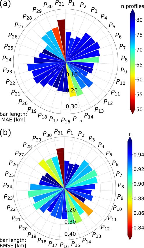
2874                                                      D. Sanchez-Rivas and M. A. Rico-Ramirez: Melting-level detection

   Knowledge of the ML is also useful for calibrating radar        thickness of the melting layer. Shusse et al. (2011) described
measurements. For instance, ZDR is prone to calibration er-        the shape and variation of the melting layer on different rain-
rors. The ML location is helpful for quantifying the bias of       fall systems and provided insights into the behaviour of ZDR
ZDR and mitigating errors in rain rate algorithms that use ZH      and ρHV during convective precipitation using C-band radar
and ZDR data (Richardson et al., 2017). Depending on the           measurements.
radar-scanning strategy, radar networks worldwide have im-            Algorithms for identifying the melting layer based on plan
plemented operational algorithms for ZDR calibration that re-      position indicator (PPI) scans have also been proposed in the
quire knowledge of the ML. Gorgucci et al. (1999) developed        literature. Brandes and Ikeda (2004) developed an empirical
a method where vertical-pointing radar observations in light       procedure based primarily on idealised profiles of ZH , linear
rain are used to calibrate ZDR , given that the shape of rain-     depolarisation ratio (LDR) and ρHV that are compared with
drops seen by the radar at 90◦ elevation is nearly circular, and   observed profiles to estimate the height of the freezing level.
therefore, ZDR measurements in light rain should be around         The estimation of the freezing-level height is refined using
0 dB. As vertical measurements sometimes are not available         equations related to precipitation intensity. Giangrande et al.
due to mechanical radar restrictions, Ryzhkov et al. (2005),       (2008) analysed the correspondence between maxima of ZH
Bechini et al. (2008) and Gourley et al. (2009), among oth-        and ZDR and minima in ρHV to estimate the boundaries of the
ers, developed algorithms for ZDR calibration analysing the        melting layer. This algorithm is tailored for scans with eleva-
interdependency between ZDR and other polarimetric vari-           tions angles between 4 and 10◦ . Later, Boodoo et al. (2010)
ables for several targets with a known – intrinsic value of        proposed an adaptation of this algorithm, varying the scan el-
ZDR , e.g. rain medium or dry snow; hence, the importance          evation and the range of values of ZH , ZDR and ρHV , making
of the ML estimation is necessary.                                 the algorithm more sensitive to less intense signatures of the
   There is a large number of papers that show the relation-       melting layer.
ship between the BB and the melting layer. Klaassen (1988)            As PPIs are the most common scans derived from oper-
modelled the melting layer and found that the BB enhance-          ational weather radars, Ryzhkov et al. (2016) proposed the
ment in the radar reflectivity (ZH ) is related to the density     quasi-vertical profile (QVP) technique to seize the benefits
of the ice particles. Fabry and Zawadzki (1995) analysed the       of PPIs. QVPs can be used for monitoring the temporal
dependency of the BB on the precipitation intensity and con-       evolution of precipitation and the microphysics of precipi-
firmed the relationship between the radar BB signatures and        tation. For instance, Kaltenboeck and Ryzhkov (2017) anal-
the melting of snowflakes in stratiform precipitation. White       ysed the evolution of the melting layer in freezing rain events
et al. (2002) introduced an algorithm based on Doppler wind        with QVP signatures, demonstrating the ability of QVPs to
profiling radar scans for detecting the BB height; their results   represent several microphysical precipitation features as the
showed a correlation between the melting layer and the peaks       dendritic growth layer and the riming region. Furthermore,
of the gradients of ZH and the radial velocity (V ) taken at       Kumjian and Lombardo (2017) and Griffin et al. (2018) in-
vertical incidence. Recently, the development of polarimetric      troduced new procedures for generating QVPs of the V and
weather radar has allowed measuring the size and thermody-         specific differential phase (KDP ) to explore the polarimetric
namic phase of precipitation particles, which has improved         signatures of microphysical processes in winter precipitation
the identification of the melting layer. For instance, Baldini     events at S-band frequencies. Despite the enormous benefits
and Gorgucci (2006) used the differential reflectivity (ZDR )      that QVPs bring in terms of improving our understanding of
and the differential propagation phase (8DP ) taken at ver-        the microphysics of precipitation, there is very little research
tical incidence to the analysis of the ML. They showed that        on the use of QVP-based algorithms for estimating the ML.
the standard deviation of these measurements, along with ZH           Most of the algorithms mentioned above require measure-
and V , are useful for the identification of the ML using C-       ments often not available from operational weather radar
band radar data.                                                   networks as weather radars cannot always perform vertical-
   Several algorithms for identifying the melting layer us-        pointing scans or produce RHI scans to observe the vertical
ing range height indicator (RHI) scans have been proposed.         structure of precipitation events. Hence, the main objective
Matrosov et al. (2007) proposed an approach for identify-          of this work is to present an automated, operational and ro-
ing the melting layer based on ρHV (correlation coefficient)       bust algorithm that can accurately detect the ML based on
measurements collected by an X-band radar. The method re-          QVPs or VPs (vertical profiles) collected from operational
lates the depressions on the ρHV profile to the melting layer,     polarimetric weather radars. The algorithm outputs are val-
with the disadvantage that the absence of such depressions         idated using ML heights from high-resolution radiosonde
hampers the application of the algorithm. Similarly, Wolfens-      data. Note that the proposed algorithm is not intended to re-
berger et al. (2016) designed an algorithm that combines ZH        place NWP-based ML estimation methods, but it is an al-
and ρHV to create a new vertical profile that enables the de-      ternative way of detecting the ML when only polarimetric
tection of strong gradients related to the boundaries of the       weather radar measurements are available. The paper is or-
melting layer for X-band radar measurements. Their results         ganised as follows. Section 2 describes the data sets used to
showed that the algorithm is efficient for characterising the      design and validate the algorithm. Section 3 examines the

Atmos. Meas. Tech., 14, 2873–2890, 2021                                             https://doi.org/10.5194/amt-14-2873-2021
D. Sanchez-Rivas and M. A. Rico-Ramirez: Melting-level detection                                                                   2875

signatures of the melting layer on both QVPs and VPs of po-
larimetric variables. Section 4 provides a detailed explana-
tion of the design of the algorithm. Results, implementation,
validation and several examples of the outputs of the algo-
rithm are presented in Sect. 5. Section 6 provides a discussion
on the performance and implementation of the algorithm. Fi-
nally, Sect. 7 provides a summary of the conclusions from
this work.

2    Data sets and methods

Radiosonde data were used to validate the ML estimated
from radar observations. The radiosonde is an instrument
that is released into the atmosphere to measure several atmo-
spheric parameters. The UK Met Office (UKMO) uses the
Vaisala RS80 radiosonde model to collect upper-air observa-
tions twice a day at different locations across the UK. The
ascent of the radiosonde extends to heights of approximately
10–30 km, and it takes measurements at 2 s intervals (Met
Office, 2007). The closest station to the selected radar site
is the Herstmonceux station (see location in Fig. 1), which
provides high-resolution radiosonde information of pressure,
temperature, relative humidity, humidity mixing ratio, sonde
position, wind speed and wind direction. As these measure-
ments provide insights for the ML location, the radiosonde         Figure 1. Location and coverage (on short pulse, SP, mode) of
data were processed to estimate the height of the 0 ◦ C wet-       the Chenies weather radar and location of the Herstmonceux ra-
bulb temperature to evaluate the algorithm performance.            diosonde station. Source: base map contains OS data. ©Crown
   The Chenies C-band operational weather radar, located in        copyright and Crown database right, 2020.
southeast England, was selected for this work. It was one of
the first UKMO radars upgraded with polarimetric capabil-          Table 1. Chenies radar characteristics.
ities (Norman et al., 2014). The radar transmits both hori-
zontally and vertically polarised electromagnetic waves si-           Chenies radar
multaneously and receives co-polar signals at the same po-            Location                      51◦ 410 21.100 N, 0◦ 310 46.900 W
larisation as that of the transmitted wave, generating mea-           Wavelength                    λ = 5.3 cm
surements such as ZH , ZDR , ρHV and 8DP . Radial velocity            Multiple elevation scans      0.5 to 90◦
(V ) measurements of the observed precipitation targets are           Beam width                    1.0◦
also available; LDR measurements are also produced for the            Pulse repetition frequency    900 Hz (SP)–300 Hz (LP)
lowest elevation scan (Met Office, 2013). The volume radar            Revolutions per minute        3.6 (SP)–1.4 (LP)
scanning strategy generates the following products:
    – A total of 5 PPI scans sampled on long pulse (LP) mode       The location and other radar characteristics are provided in
      (pulse length is equal to 2000 µs; range covered is equal    Table 1 and Fig. 1.
      to 250 km) at 0.5, 1, 2, 3 and 4◦ elevation angles, with a      Polarimetric scans related to precipitation events through-
      600 m gate resolution every 5 min.                           out 2018 were analysed for the design and evaluation of the
    – A total of 5 PPI scans sampled on short pulse (SP) mode      algorithm. To reduce the probability of ground clutter con-
      (pulse length is equal to 500 µs; range covered is equal     tamination and beam spreading effects, only SP scans from
      to 115 km) at 1, 2, 4, 6 and 9◦ elevation angles, every      the 4, 6, 9 and 90◦ elevations angles were retained for fur-
      10 min, with the same gate resolution as above.              ther processing. Then, a pre-processing of the raw radar data
                                                                   is carried out to discard non-meteorological echoes and con-
    – A single SP PPI scan at vertical incidence (range cov-       struct the profiles of polarimetric variables as follows:
      ered is equal to 12 km) every 10 min, with 75 m gate
      resolution.                                                    – For the 4, 6 and 9◦ elevation scans, remnant clutter
                                                                       and anomalous propagation echoes were removed using
    – A single PPI scan with LDR measurements every 5 min              the algorithm proposed by Rico-Ramirez and Cluckie
      at the lowest elevation (0.5◦ ).                                 (2008), specifically calibrated with data from this radar.

https://doi.org/10.5194/amt-14-2873-2021                                              Atmos. Meas. Tech., 14, 2873–2890, 2021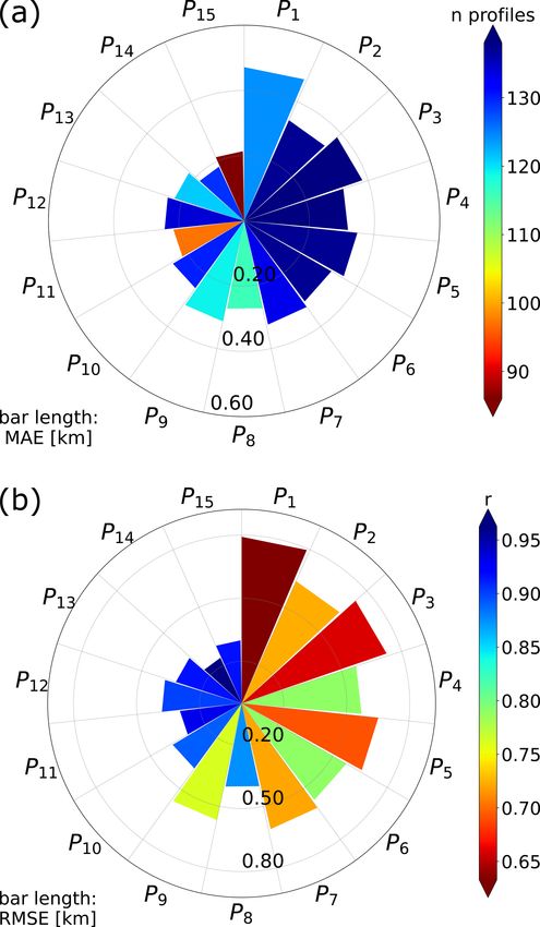
2876 D. Sanchez-Rivas and M. A. Rico-Ramirez: Melting-level detection
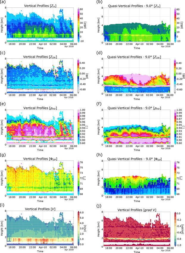
Then, following the procedure suggested by Ryzhkov 3 Polarimetric signatures of the melting layer
et al. (2016), we generated QVPs of ZH , ZDR , ρHV
and 8DP measurements. The procedure suggests the az- The VPs and QVPs of the polarimetric measurements are dis-
imuthal averaging of the polarimetric measurements at played in height versus time plots. This enables the visualisa-
high-elevation scans (10–30◦ ), but such elevation angles tion of the temporal evolution of the polarimetric radar signa-
were not available on our data sets; hence, we used the tures in the melting layer. Figure 2 depicts a stratiform rain-
highest elevation angles available to generate the QVPs. fall event recorded between 9 and 10 April 2018 using VPs
Although it is possible to produce time-averaged QVPs and QVPs (9◦ elevation angle). It can be seen that every radar
to avoid local storm effects, we decided to keep the variable exhibits distinctive features that provide unique in-
original time resolution of the QVPs; therefore, we pro- formation for the identification of the melting layer on both
duced one QVP for each PPI scan. Details on the con- VPs and QVPs; e.g. Fig. 2a–b and c–d exhibit regions of en-
struction of the QVPs are provided in Sect. 6. hanced values of ZH (BB) and ZDR , respectively, that are
visible just below 2 km in height. Concurrently, Fig. 2e–f
– For the scans taken at vertical incidence, the data re- and g–h show that ρHV and 8DP are sensitive to the phase
lated to the first kilometre above ground level (a.g.l.) are and shape of hydrometeors, while Fig. 2i shows that the fall
not usable due to some inherent radar limitations, e.g. velocities of snow particles are lower compared to rain parti-
the de-ionisation time of the transmit–receive (TR) cell cles, which is an important feature that can be used to detect
(Timothy Darlington, Met Office, personal communica- the ML. Figure 2j shows the gradient of the radial velocity
tion, 2019) or clutter contamination. After discarding (gradV ) generated from 90◦ elevation scans, where the BB
the data below this height, an azimuthal averaging of the enhancement is clearly visible at 2 km in height, and it is re-
polarimetric and radial velocity data collected at vertical lated to the increase in the fall velocities of the hydrometeors.
incidence was performed, generating VPs of ZH , ZDR , The different BB signatures expected in the melting layer on
ρHV , 8DP and V . For the analysed radar data sets, the the QVPs and VPs are explained next.
spectral width variable was not available. We also de- For comparison purposes, Fig. 3 shows normalised ver-
fine a new variable, the radial velocity gradient (gradV ), sions of VPs and QVPs (scaling each profile into the range [0,
computed using the gradient of the 90◦ radial velocity 1]) taken from the stratiform event presented in Fig. 2; also,
profile (note that gradV ≡ dV /dH ). This new variable the height of the 0 ◦ C wet-bulb isotherm is shown. The nor-
accentuates the profile extremes related to the change malisation process intensifies the signatures of the melting
in the hydrometeor fall velocities from ice or snow to layer. Note that the QVPs provide information below 1 km;
rain. The gradient of V is computed using first-order this is important for the analysis of showers or events with
central differences in the interior points and first-order ML at relatively low altitude.
forward or backwards differences at the boundaries; for Given that the main objective of this work is to detect the
an in-depth description of numerical differentiation and melting layer boundaries based on the geometric features of
finite-differences methods, see Moin (2010). the polarimetric profiles, herein, we will try to explain how
Regarding the attenuation corrections needed for ZH and the melting layer shapes the structure of the radar profiles.
ZDR , for most of the scans used in this work (especially 90 Figure 3 shows the presence of enhancements on the po-
and 9◦ elevation scans) we observed that rain attenuation was larimetric profiles related to the variation in the phase and
relatively small after analysing the total differential phase concentration of the hydrometeors. Taking the 0 ◦ C wet-bulb
shift. Furthermore, the ML height is essential for implement- height as a reference (just below 2 km in altitude), it is feasi-
ing rain attenuation correction algorithms. Hence, no attempt ble to associate the upper boundaries of these enhancements
was made to correct for attenuation. to the ML. These enhancements are not necessarily at the
Based on the constructed VPs and QVPs, a total of 94 rain- same height in all polarimetric variables, but this has to do
fall events, with visible signatures of the melting layer on ZH with the backscattering properties of the melting particles
or ρHV , were selected, i.e. an enhancement up to 30 dBZ on and their relationship with the measured variable. Also, it
ZH or ρHV constantly decreasing below 0.90. Also, from the is important to highlight that the methods used in the con-
total number of rain events, only 25 events observed by the struction of the profiles play a key role in the location of the
radar showed a suitable temporal matching with the data col- peaks, i.e. both VPs and QVPs result from an azimuthal av-
lected by the radiosondes, i.e. the difference in time between eraging of the rays, representing an average structure of the
radar and radiosonde measurements do not exceed 2 h. This storm that helps to enhance the BB signature. So, the BB
time window was set to minimise the impact of the variability peaks in the VPs and QVPs in all radar measurements differ
of the height of the ML. from the instantaneous profiles observed at individual slant
ranges; this will be discussed in Sect. 6.
The reflectivity (ZH ) represents the power backscattered
by precipitation particles, thus providing information about
the concentration, size and phase of the hydrometeors
Atmos. Meas. Tech., 14, 2873–2890, 2021 https://doi.org/10.5194/amt-14-2873-2021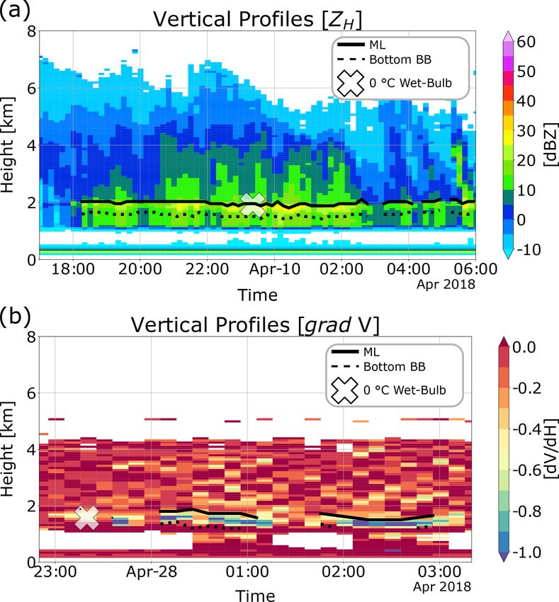
D. Sanchez-Rivas and M. A. Rico-Ramirez: Melting-level detection                                                                         2877

Figure 2. Height versus time plots of ZH (a–b), ZDR (c–d), ρHV (e–f) and 8DP (g–h), generated from VPs (left) and QVPs (right) for a pre-
cipitation event recorded by a weather radar located at Chenies, UK. Also, panel (i) portrays the radial (vertical) velocity V of hydrometeors,
whilst panel (j) shows a plot of the profiles based on the gradient of V measurements [dV /dH ].

(Hong and Gourley, 2015). In Fig. 2a and b, it can be seen                change in size from large melting snowflakes to raindrops
that the values of ZH on both QVPs and VPs show similar                   and by the increase in the fall speed of the hydrometeors that
intensities. Also, the well-known BB effect on ZH is visible              reduce the particle concentration (Fabry, 2015). The BB is
on both profiles (around 1.7 km). The BB is caused by the                 easily observed in stratiform events; however, it is difficult
increase in the dielectric constant of melting particles, by the          to set the melting layer boundaries based only on ZH ; e.g. in

https://doi.org/10.5194/amt-14-2873-2021                                                     Atmos. Meas. Tech., 14, 2873–2890, 2021
2878                                                      D. Sanchez-Rivas and M. A. Rico-Ramirez: Melting-level detection

Figure 3. Normalised version of VPs and QVPs generated from polarimetric scans recorded at different elevation angles, related to a
stratiform-type rain event. The 0 ◦ C wet-bulb height is shown with the dashed–dotted line.

Fig. 3a, the top of the BB is not easy to discern. Moreover,        et al., 1999). A subsequent analysis of birdbath scans in light
the profiles of ZH do not show the BB feature in convective         rain through the whole data set confirmed a persistent off-
events; therefore, the estimation of ML for convective events,      set in ZDR . This reaffirms the importance of the detection of
based only on ZH , is not feasible.                                 the melting layer boundaries, as it helps to set limits for the
   The differential reflectivity (ZDR ) represents the ratio be-    implementation of a ZDR calibration algorithm.
tween horizontal and vertical reflectivity values (ZH /ZV ),           The correlation coefficient (ρHV ) measures the correlation
and it is related to the orientation, shape and size of the hy-     between the backscatter amplitudes at vertical and horizontal
drometeors (Islam and Rico-Ramirez, 2014); therefore, ZDR           polarisations. It is sensitive to the distribution of particle sizes
measurements for QVPs and VPs may describe different fea-           and shapes and, hence, sensitive to the hydrometeors phase,
tures of the particles as the elevation angle varies. For both      becoming a valuable hydrometeor classifier for identifying
QVPs and VPs, ZDR profiles show similar behaviour in strat-         non-meteorological echoes (Islam and Rico-Ramirez, 2014).
iform events. Figure 3b shows that ZDR exhibit mean small           Additionally, ρHV is a reliable indicator of the quality of the
slope changes on the rain medium (below 1.2 km), but there          radar data as, in the rain medium, the correlation is close to
is a noticeable peak associated with the melting layer on           1, becoming an indicator of the quality of the polarimetric
both VPs and QVPs, and although there is a difference in            radar measurements (Kumjian, 2013a). Figure 2e and f show
the peak height between both types of profiles, the top and         that ρHV is close to one within the rain region, which con-
bottom boundaries are at similar heights, especially for the        firms the high quality of this radar data set. Figure 3c shows
QVPs. Brandes and Ikeda (2004) and Ryzhkov et al. (2016)            that the melting layer causes a similar response on ρHV as
showed that the presence of melting, randomly oriented ice          in ZH and ZDR , but in the opposite direction, resulting in a
particles within the melting layer and the mixing of hydrom-        depression on the profiles starting at 1.4–1.5 km in height for
eteors produce the peaks in ZDR in stratiform events. How-          QVPs and VPs, respectively. This depression results from the
ever, for profiles related to convective events (not shown),        shift between high values of ρHV , related to raindrops and ice
the VPs sometimes exhibit an inverse peak exactly above the         crystals and lower values triggered by the variety of shapes
rain medium and then generate a noisy, random pattern on            and axis ratios of the hydrometeors (Kumjian, 2013b). The
the melting layer that makes the estimation of the ML more          behaviour of ρHV is similar on both VPs and QVPs from 9◦
difficult when using VPs of ZDR . Finally, the most signifi-        elevation for stratiform or convective events, where the major
cant difference for this variable can be seen in Fig. 2c and d,     difference lies in the depth of the depressions. This may be
where the values of ZDR for VPs and QVPs differ from each           caused by the resolution and elevation angle of the original
other, especially in the melting layer and above. It is also im-    scans. On the other hand, the QVPs constructed from lower
portant to highlight that ZDR provides valuable information         elevation angles, i.e. 4 and 6◦ , exhibit less pronounced peaks
for QPE. However, it usually shows a bias that must be cor-         related to the melting layer, and a pronounced decrease in
rected; e.g. in Fig. 2c there is a bias in ZDR (∼ −0.35 dB) as      ρHV above the BB that can make it difficult to identify the
we expect near-to-zero values for ZDR in the rain region for        ML.
vertically pointing measurements, as raindrops are symmet-             As can be seen in Figs. 2g–h and 3d, the signatures of the
rical on average when observed from underneath (Gorgucci            melting layer on the differential propagation phase (8DP )

Atmos. Meas. Tech., 14, 2873–2890, 2021                                               https://doi.org/10.5194/amt-14-2873-2021
D. Sanchez-Rivas and M. A. Rico-Ramirez: Melting-level detection 2879
are, to a certain degree, ambiguous in our data sets, espe-
cially on the QVPs. 8DP represents the difference between
the phase of the radar signal at horizontal and vertical polar-
isation, providing valuable information about the shape and
concentration of the hydrometeors (Islam and Rico-Ramirez,
2014). Hence, the peaks on this type of profile may be related
to a greater concentration of particles due to the presence of
the melting layer or the dendritic growth layer (DGL), as pre-
viously explored by Griffin et al. (2018), Kaltenboeck and
Ryzhkov (2017) and Ryzhkov et al. (2016). Figure 3d shows
that the QVPs of 8DP from 9◦ elevation exhibit a small peak
at 1.7 km in height related to the melting layer, but it is not as
pronounced as with the other polarimetric variables, although
there are significant peaks aloft (between 2.8 and 3.8 km)
that may represent particle (ice or snowflakes) alignment on
the DGL, as suggested by Kaltenboeck and Ryzhkov (2017),
while lower elevation angles do not show strong signatures
on the melting layer or the DGL. In contrast, for 90◦ eleva-
tion scans, there is a well-defined depression in 8DP related
to melting and particle growth (Brandes and Ikeda, 2004) at
1.8 km in height that closely matches the height of the BB;
regarding the signatures of the DGL on the VPs, due to the
noisiness of the profile above the ML, it is difficult to deter-
mine if these peaks are related to the DGL.
Figures 2i and 3e show the profiles related to the radial
(vertical) velocities (V ) and the signatures of the melting
layer on this variable. It can be seen that the fall velocity
of the hydrometeors is relatively constant and close to zero
above the ML, which is related to the fall velocity of ice and
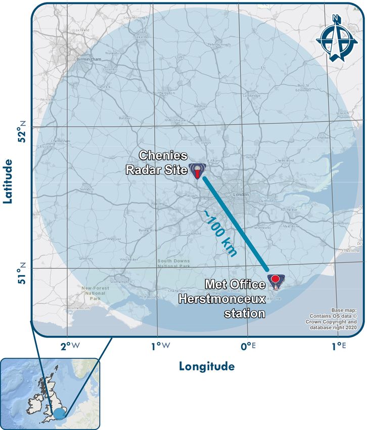
snow particles; then, there is a sharp increase in the fall veloc- Figure 4. Flow chart of the proposed MLA.
ity of the precipitation particles in the melting layer that be-
comes constant again in the rain region. However, it is chal-
lenging to incorporate the velocity profile into the ML de- puts of the algorithm, in combination with radiosonde data,
tection because its features are not easy to identify using an determines the combination of radar signatures that is the
automated peak search algorithm. Conversely, the VP of the best predictor of the ML. Some considerations are made for
radial (vertical) velocity gradient (gradV ), shown in Figs. 2j its design; for example, to minimise the effect of beam broad-
and 3e (dotted line), exhibits a BB enhancement and peak ening, the analysis is constrained to a height of 5 km (for 9◦
similar to the rest of polarimetric variables, where the upper scans, the height of the centre of the beam is similar to 30 km
and lower curvatures of the peak match the top and bottom in range). Also, as shown in Fig. 3, some profiles become
extents of the melting layer. noisy above the ML or contain spurious echoes aloft, mak-
ing it necessary to set an initial upper extent for the algo-
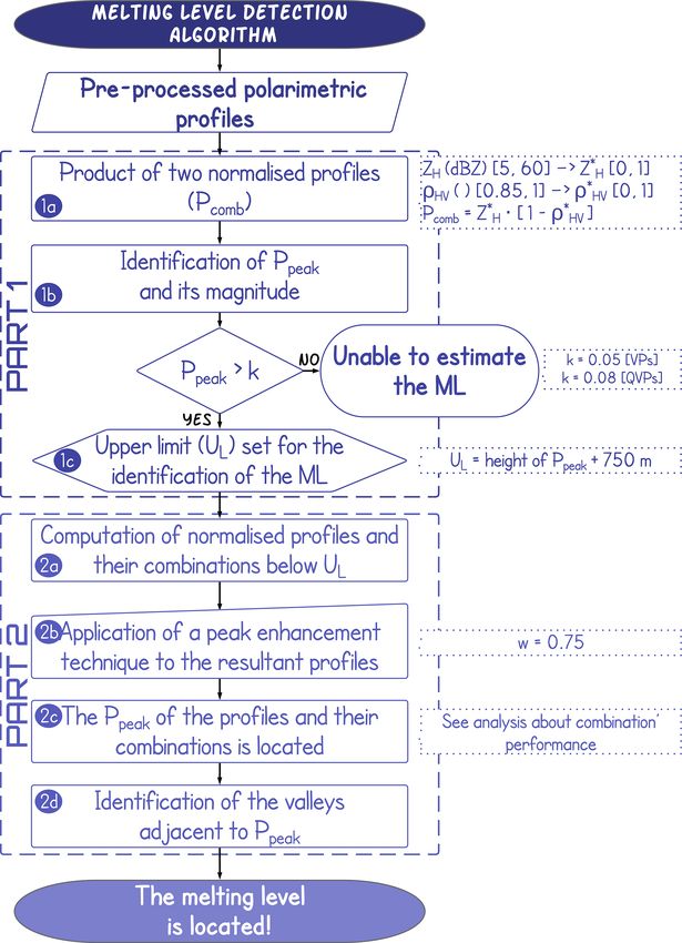
rithm to work. The MLA is divided into two parts. The first
4 Algorithm to identify the melting level part determines if the profile contains elements for detecting
the melting layer based on the combination of two profiles
The melting level algorithm (MLA) automatically detects the and setting an upper limit for its implementation. The second
ML, using either QVPs or VPs, under the premise that the part estimates the ML based on a combination of the polari-
peaks on each polarimetric profile and their curvatures are metric profiles and their features. The algorithm uses either
related to the melting layer. The MLA is based on the pro- QVPs or VPs, but we avoid combining both profiles, as VPs
cedure proposed by Wolfensberger et al. (2016) that com- might not be available in other weather radar networks. A
bines ZH and ρHV to create a new profile with enhanced flow chart that illustrates the MLA steps is shown in Fig. 4
melting layer features. However, Fig. 3 shows that there are and described below.
additional variables, such as gradV , that may improve the
identification of the ML. Therefore, we propose an algorithm
that combines all the various radar signatures to estimate the
melting layer boundaries. A subsequent analysis of the out-
https://doi.org/10.5194/amt-14-2873-2021 Atmos. Meas. Tech., 14, 2873–2890, 2021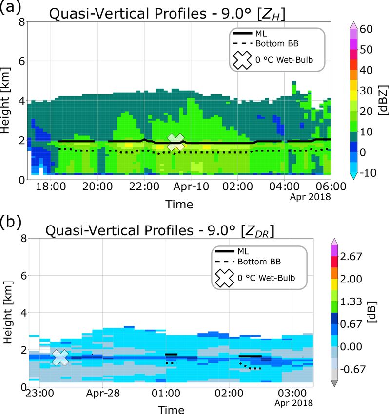
2880                                                                               D. Sanchez-Rivas and M. A. Rico-Ramirez: Melting-level detection

Table 2. Possible combinations of polarimetric variables for VPs and QVPs used for the ML detection.

  (VPs)               (QVPs)          P1        P2       P3        P4        P5      P6    P7     P8        P9   P10   P11    P12    P13   P14    P15
  1 − gradV ∗         –                ◦         ◦        ◦         ◦         ◦       ◦    ◦       ◦        ◦     ◦     ◦      ◦      ◦      ◦      ◦
  ZH∗                 ZH∗              ◦         ◦        ◦         ◦         ◦       ◦    ◦       •        •     •     •      •      •      •      •
    ∗
  ZDR                   ∗
                      ZDR              ◦         ◦        ◦         •         •       •    •       ◦        ◦     ◦     ◦      •      •      •      •
       ∗
  1 − ρHV                  ∗
                      1 − ρHV          ◦         •        •         ◦         ◦       •    •       ◦        ◦     •     •      ◦      ◦      •      •
  1 − 8∗DP              ∗
                      8DP              •         ◦        •         ◦         •       ◦    •       ◦        •     ◦     •      ◦      •      ◦      •
  (VPs)               (QVPs)          P16      P17      P18       P19        P20    P21   P22     P23    P24     P25   P26    P27    P28   P29    P30    P31
  1 − gradV ∗         –                •         •        •         •         •       •    •       •        •     •     •      •      •      •      •      •
  ZH∗                 –                ◦         ◦        ◦         ◦         ◦       ◦    ◦       ◦        •     •     •      •      •      •      •      •
    ∗
  ZDR                 –                ◦         ◦        ◦         ◦         •       •    •       •        ◦     ◦     ◦      ◦      •      •      •      •
       ∗
  1 − ρHV             –                ◦         ◦        •         •         ◦       ◦    •       •        ◦     ◦     •      •      ◦      ◦      •      •
  1 − 8∗DP            –                ◦         •        ◦         •         ◦       •    ◦       •        ◦     •     ◦      •      ◦      •      ◦      •

Note: The asterisk (∗ ) refers to the normalised version of the variables.

  1. Part 1                                                                                             in the profile, the peak with the higher magnitude
       The first part of the MLA identifies profiles that are                                           (i.e. the horizontal distance between the peak and
       likely to contain signatures related to the melting layer                                        the origin) is set as Ppeak . Then, to identify profiles
       and sets an upper limit in the profiles to use all the avail-                                    with a Ppeak strong enough to be related to poten-
       able variables.                                                                                  tial melting layer signatures, a threshold, k, is set.
                                                                                                        If the magnitude of Ppeak is less than the thresh-
       1a. The algorithm takes advantage of the distinctive                                             old, k (set to 0.05 for VPs and 0.08 for QVPs), the
           signatures on the profiles of ZH and ρHV , on both                                           MLA determines that the gradients are not strong
           VPs and QVPs, to perform an initial identification                                           enough to correspond to melting layer signatures,
           of rain echoes. These two profiles are normalised                                            and therefore, the profile does not contain elements
           and combined into a single profile (Pcomb ), as sug-                                         for detecting the ML. This step is illustrated in
           gested by Wolfensberger et al. (2016), but using dif-                                        Fig. 5a, where the magnitude of Ppeak (∼ 0.14) is
           ferent thresholds for ZH and ρHV related to drizzle,                                         greater than the threshold, k. Further discussion on
           heavy rain, snow and ice (Kumjian, 2013a; Fabry,                                             the value of this parameter is provided in Sects. 4.1
           2015). Hence, values of ZH , between 5 and 60 dBZ,                                           and 6.
           and ρHV , between 0.85 and 1, are normalised to                                         1c. If the magnitude of Ppeak is greater than k, an up-
           0 and 1 as follows: [ZH (dBZ)[5, 60] → ZH     ∗ [0, 1]]
                                        ∗
                                                                                                       per limit (UL ) is set, taking the height of Ppeak
           and [ρHV ( )[0.85, 1] → ρHV [0, 1]]. Values outside                                         and adding 750 m above. This value is selected as
           these intervals are fixed to 0 and 1, correspondingly.                                      the melting layer thickness usually reaches values
           The normalisation is carried out using the min–max                                          less than about 800 m (Fabry and Zawadzki, 1995);
           normalisation procedure. Then, the normalised pro-                                          hence, 750 m is sufficient for refining the search of
           files are combined using the complement of ρHV to                                           the ML. Figure 5a illustrates this step, where 750 m
           enhance the peaks present in the profiles as follows:                                       are added to the height of Ppeak (∼ 1.51 km) to set
                       ∗          ∗
                                                                                                      an upper limit (∼ 2.26 km).
           Pcomb = ZH    · 1 − ρHV    .                        (1)
                                                                                                2. Part 2
              Note that the asterisk (∗ ) refers to a normalised vari-
              able.                                                                                In the second part of the algorithm, we incorporate the
              The profile Pcomb is likely to show an enhanced                                      rest of the polarimetric variables to analyse their ca-
              peak if potential melting layer signatures were                                      pability for refining the detection of the melting layer
              present in the profiles of ZH and ρHV .                                              boundaries and determining the combination that better
                                                                                                   detects the ML.
       1b. The MLA locates the peaks on the profile Pcomb by
           comparing neighbouring values. A peak is a sample                                       2a. In this step, the profiles of all the radar variables are
           for which the direct neighbours have smaller mag-                                           cut below UL . Then, and considering that ZH       ∗ and

           nitudes. Inversely, the valleys (or boundaries of the                                         ∗
                                                                                                       ρHV were already normalised in step 1a, the other
           peaks) within the profile can also be detected using                                        variables are also normalised but use the minimum
           a similar rationale. As several peaks can be present                                        and maximum values in each profile as thresh-

Atmos. Meas. Tech., 14, 2873–2890, 2021                                                                          https://doi.org/10.5194/amt-14-2873-2021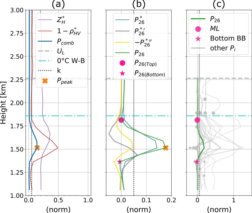
D. Sanchez-Rivas and M. A. Rico-Ramirez: Melting-level detection                                                                2881

         olds. To incorporate all the variables into the al-
         gorithm, the complement of the variables is used
         when appropriate. This is made to generate profiles
         with analogue peaks that enhance the footprints of
         the melting layer when combined with other vari-
         ables. Equations (2) and (3), respectively, are de-
         rived based on the patterns observed in VPs and
         QVPs. These equations vary according to the com-
         bination of the variables presented in Table 2.

         Pi∗ = 1 − gradV ∗ · ZH    ∗       ∗

                                       · ZDR
                     ∗
                          · 1 − 8∗DP

             · 1 − ρHV                                   (2)
         Pi∗ = ZH ∗        ∗            ∗
                                            · 8∗DP ,

                      · ZDR    · 1 − ρHV                 (3)

         where i depends on the combination of the vari-
         ables used according to Table 2.
         The algorithm computes all the possible combina-
         tions of the profiles to analyse the influence of each
         variable by, in this case, generating 31 different pro-   Figure 5. Depiction of the implementation of the algorithm for ML
         files if using VPs and 15 profiles when using QVPs.       detection.
     2b. The profiles (Pi∗ ) generated in the previous step
         will very likely show a peak related to the melt-
         ing layer. The next step in the MLA is to apply a         ful for detecting the presence of the melting layer. An ad-
         peak enhancement technique to refine the bound-           equate choice of the magnitude of the parameter (k) is im-
         aries of this peak. This can be done using the fol-       portant to discard profiles with a Ppeak that is not strong
         lowing equation:                                          enough to be related to the melting layer. However, addi-
                                                                   tional variables can be used (see Eqs. 2 and 3) to refine
         Pi = Pi∗ − w · Pi∗00 ,

                                                         (4)       the detection of the ML. The upper limit (UL ) allows the
                                                                   use of other variables that otherwise could not be part of
         where Pi is the enhanced profile, Pi∗ is the pro-         the algorithm due to noisiness or spurious echoes present
         file given by Eqs. (2) or (3), w is a weighting fac-      at the top of the profiles. Figure 5b shows the importance
         tor, and Pi∗00 is the second derivative of Pi∗ . The      of the refinement of the profile, e.g. the profile combination
         optimum choice of the parameter w depends upon              ∗ = (1 − gradV ∗ ) · (Z ∗ ) · (1 − ρ ∗ ) (blue line) has a peak
                                                                   P26                        H           HV
         the signal-to-noise ratio and the desirable sharpen-      related to the melting layer, and the valley located at the top
         ing extent. Table 2 lists the enhanced profiles pro-      of this peak is close to the ML, but it is difficult for a peak
         duced by combining different polarimetric profiles,       detection algorithm to detect its height, as it is not as pro-
         and Fig. 5b shows the enhancement of the peak and         nounced as required. The use of the first derivative of the
         valleys. Details on the value of the parameter w are                     ∗0 (grey line), is not helpful, as the peaks are not
                                                                   profile, i.e. P26
         presented in Sects. 4.1 and 6.                            close to the ML. The profile P26 (green line) results from the
     2c. For each profile Pi , the maximum enhancement in          implementation of Eq. (4), where a value of w equal to 0.75
         the BB has a magnitude given by Ppeak and com-            enhances the peak and its valleys enough for the algorithm
         puted as in step 1b. Then the parameter k is used to      to detect their boundaries. A proper choice of the parameter
         discard profiles with peaks not related to the melt-      w depends on the desired weight to the original profile rather
         ing layer (k = 0.05 for VPs; k = 0.08 for QVPs).          than its second derivative. The impact of the parameters k
    2d. The top and bottom boundaries of the BB enhance-           and w on the algorithm is discussed in the following section.
        ment in Pi can be placed by searching the inverse
        peaks (valleys) directly above and below Ppeak . Fi-       4.1   Implementation of the ML algorithm
        nally, the algorithm allocates these points as being
        the boundaries of the melting layer. This step is          As described before, the MLA performs a pre-classification
        shown in Fig. 5c, where the selected profile P26 is        of profiles likely to contain melting layer signatures. Some
                                                                   tests were carried out by replacing ZH   ∗ with other variables
        highlighted. The top valley of Pi is set as the esti-                              ∗
        mated height of the ML (MLTop ).                           (e.g. ZDR or 1−gradV ) to identify improvements in the pre-
                                                                   classification. From Fig. 3b, it is clear that the QVPs of ZDR
  As can be seen in Fig. 5a, the combination of ZH    ∗ and        exhibit a pronounced peak related to the melting layer, even
     ∗
1 − ρHV produces a profile with a peak (Ppeak ) that is use-       for low elevation angles, but unfortunately, ZDR is not cali-

https://doi.org/10.5194/amt-14-2873-2021                                              Atmos. Meas. Tech., 14, 2873–2890, 2021
2882 D. Sanchez-Rivas and M. A. Rico-Ramirez: Melting-level detection
brated, and the thresholds for normalising this variable may
vary depending on the elevation angle. On the other hand,
replacing ZH ∗ with the profile 1 − gradV ∗ for the VPs could
improve the pre-classification, but this may restrict the imple-
mentation of the algorithm, i.e. it would be only applicable
if vertical velocity profiles are available. Although we ob-
served some improvements using these variables in the first
part of the MLA, especially for rain showers, we wanted to
keep this part as simple and robust as possible to enable the
reproducibility of the algorithm. Hence, we used the combi-
∗ and ρ Figure 6. Comparison of VPs and QVPs of ZH generated at two el-
nation of ZH HV for part 1 of the algorithm, as initially
evation angles for a collection of stratiform events. Counts indicate
proposed by Wolfensberger et al. (2016).
the number of points in the hexagon.
On the other hand, the algorithm relies on the parameters
k and w, as shown in Fig. 5a and b. These parameters can be
adjusted according to the radar data sets, e.g. the parameter
k can be affected by the quality of ρHV . In our data sets, and
after the removal of non-meteorological echoes, ρHV exhibits
values close to 0.85 in the melting layer on both QVPs and
VPs, but this may vary depending on the type of radar, scan-
ning strategy and quality of the data sets. We set k equal to
0.05 for VPs and k equal to 0.08 for QVPs empirically, and
these values allow the algorithm to discard enhancements in
the profile not related to the melting layer. Moreover, several Figure 7. As in Fig. 6 but for a collection of convective events.
tests were carried out using time-averaged QVPs, resulting in Counts indicate the number of points in the hexagon.
smoother profiles, and this parameter was helpful for iden-
tifying profiles with melting layer signatures. On the other
hand, Eq. (4) is applied to the profiles to enhance the BB as this is the variable less prone to significant variations due
peak and the top and bottom boundaries (i.e. valleys) within to the elevation angle. For the rest of the variables, it is not
the profile, thus refining the detection of the ML. This equa- possible to compare QVPs as their characteristics vary with
tion combines the original profile with its second derivative, the elevation angle used to build the QVPs.
weighted with the parameter w. As shown in Fig. 5b, the To carry out this analysis, we manually classified the rain
second derivative of the profile (yellow line) exhibits deeper events recorded by the radar according to the recommenda-
peaks, but its top boundary is still far from the measured ML. tions of Fabry and Zawadzki (1995) and Rico-Ramirez et al.
After several trials, we set w equal to 0.75, as this value en- (2007). From a total of 94 rainfall events, 68 events were
hances the peaks of the original profile without compromis- classified as stratiform. This category includes low-level rain
ing the match of the top boundary and improving the ML and rain with BB, as they showed the well-known enhance-
detection. Likewise, this parameter can be adjusted depend- ment of reflectivity observed within the melting layer or
ing on the radar data sets, e.g. profiles that exhibit smoother look-alike drizzle events below the 0 ◦ C. On the other hand,
peaks due to the nature of its construction process and the 26 events recorded mainly during the summer met the char-
resolution of the original scans, or profiles with vertical res- acteristics of showers, i.e. indistinguishable signatures of the
olution too coarse can be adjusted with the parameter w for melting layer in the ZH profiles, in which higher values of
a better algorithm performance. reflectivity are present; the latter is the type of precipitation
less common in the UK (Collier, 2003). The comparison be-
tween VPs and QVPs takes into account the timestamp and
5 Results spatial resolution of the profiles. The Pearson correlation co-
efficient (r) is computed to analyse the consistency between
5.1 VP and QVP comparison the VPs and QVPs. The results for stratiform and convective
events are shown in Figs. 6 and 7, respectively.
Both VPs and QVPs proved to be an efficient way of mon- Figure 6 shows that reflectivity values related to light and
itoring the temporal evolution of the melting layer, but the moderate rain rates (expected on stratiform-type events) are
elevation angle used to build the QVPs affects each radar similarly depicted on both VPs and QVPs. However, the
variable in different ways, as described in Sect. 3 and shown agreement diminishes when decreasing the elevation angle,
in Figs. 2 and 3. Hence, to support the performance and out- mainly because higher values of ZH do not always match
puts of the algorithm, we assessed the consistency between their pairs as the elevation decrease. This could be explained
the ZH profiles constructed from different elevation angles, by the averaging process carried out in the construction pro-
Atmos. Meas. Tech., 14, 2873–2890, 2021 https://doi.org/10.5194/amt-14-2873-2021D. Sanchez-Rivas and M. A. Rico-Ramirez: Melting-level detection 2883
cess of the profiles, as the radar resolution volume increases
with distance. On the other hand, Fig. 7 shows a more scat-
tered distribution of ZH for shower-type events in which
higher values of ZH (related to moderate to heavy rain rates)
are present. Again, the correlation decreases for lower ele-
vation angles, and it can be seen that there are mismatches
for cells with higher values of reflectivity. This can be re-
lated to local storm effects and spatially nonuniform convec-
tive elements present in the QVPs, as explored by Ryzhkov
et al. (2016). It is worth mentioning that QVPs constructed
from lower elevation angles were also assessed (results not
shown), but similar behaviour was observed, e.g. correlation
decreases even further. Also, a similar analysis was carried
out using other polarimetric variables. However, the results
were not consistent as only ZH describes similar properties
of the precipitation measurements taken at these elevation an-
gles.
5.2 ML detection from VPs
The MLA outputs were analysed to find the combination of
VPs that better detects the ML. These outputs are compared
against 0 ◦ C wet-bulb isotherms over 1 year of rainfall events.
Since soundings are released twice daily, the radiosonde data
are extended at several time steps to create short time win-
dows and enable a comprehensive comparison with the radar
data. Performance metrics (Pearson correlation coefficient – Figure 8. Errors in the ML detection for VPs using a ±30 min win-
r; mean absolute error – MAE; root mean square error – dow. In panel (a), the bar length represents the MAE (in kilometres),
RMSE) between the height of the 0 ◦ C wet-bulb isotherm and colour represents the number of vertical profiles with strong
signatures detected by every polarimetric combination; in panel (b),
and the estimated ML are computed. Figure 8 shows the re-
the bar length represents the RMSE (in kilometres) for every polari-
sults for a 60 min window, i.e. the height of the 0 ◦ C wet- metric combination, and colour represents the Pearson correlation
bulb isotherm is assumed constant 30 min before and after coefficient.
the timestamp of the radiosonde.
Figure 8 shows the capabilities of all polarimetric vari-
ables for the detection of the ML. In Fig. 8a, the variable n and its steadiness regarding the ML. Examples of the detec-
profiles is an indicator of the number of profiles that, accord- tion of the melting layer for stratiform and convective events
ing to the algorithm, contain peaks strong enough to be re- using the profile P26 are shown in Fig. 10. Figure 10a and
lated to the melting layer. This variable can only be validated b show the output of the MLA using the combination P26
by a visual inspection of the algorithm outputs, as some vari- in both stratiform or convective events. The algorithm shows
ables may incorrectly classify some peaks as being melting a good performance, especially for stratiform events where
layer related. Overall, Fig. 8 shows that the combinations that the ML height and the rain zone are accurately defined. For
include ZH ∗ , [1 − ρ ∗ ] or [1 − gradV ∗ ] improve the accuracy
HV the convective event, the ML is correctly identified, although
of the MLA, e.g. P9 , P11 or P26 , as the correlation, and the er- the bottom of the melting layer is not entirely detected. This
rors are relatively low for these combinations. After a visual is a drawback when using the algorithm based on VPs and
assessment of the performance of each combination and sup- highlights the problems when low-altitude melting layers are
ported by the statistics computed above, we determine that present.
the profile combination P26 = [ZH ∗ ·(1−ρ ∗ )·(1−gradV ∗ )]
HV
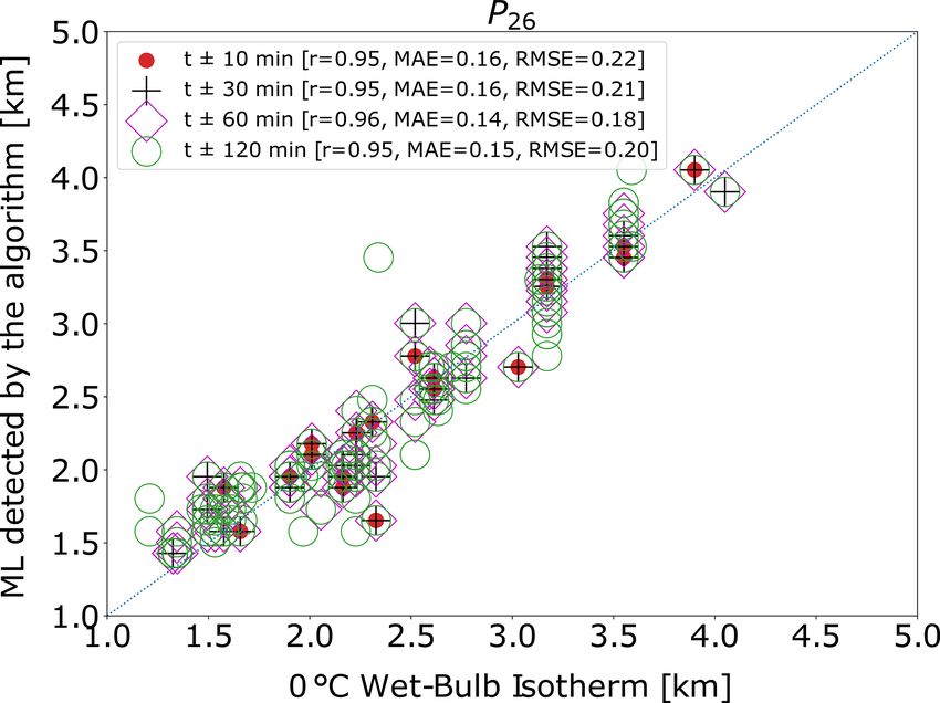
is the best predictor of the ML. Then, several time windows 5.3 ML detection from QVP
are set to assess the accuracy of the MLA over 1 year of
radar data, as shown in Fig. 9. This analysis confirms the The MLA is applied to QVPs generated from scans at three
good performance of the combination P26 on the ML detec- different elevation angles (4, 6 and 9◦ ). After several tri-
tion, even when increasing the time window, as the RMSE als on the parameters k and w in the algorithm implemen-
and MAE are close to 200 m and r equals 0.95. Another in- tation, only the highest elevation produced satisfactory ML
dicator taken into account in the visual inspection of the al- estimation results. The explanation of this has its foundation
gorithm output was the detection of the melting layer bottom in Fig. 3c, where QVPs from lower elevation angles display
https://doi.org/10.5194/amt-14-2873-2021 Atmos. Meas. Tech., 14, 2873–2890, 20212884 D. Sanchez-Rivas and M. A. Rico-Ramirez: Melting-level detection
Figure 9. Heights of the 0 ◦ C wet-bulb isotherm versus ML detected
by the algorithm using the combination P26 for several time win-
dows. The 1 : 1 line is shown in blue. MAE and RMSE are shown
in kilometres.
Figure 11. Errors in the ML detection for QVPs using a ±30 min
window. In panel (a), the bar length represents the MAE (in kilome-
tres), and colour represents the number of QVPs with strong signa-
tures detected by every polarimetric combination; in panel (b), the
bar length represents the RMSE (in kilometres) for every polari-
metric combination, and colour represents the Pearson correlation
coefficient.
k cannot correctly filter gradients related to the ML. Thus,
after several trials, and supported by the analysis presented
in Sect. 5.1, we decided not to use the lower elevation an-
gles (4 and 6◦ ). Using the same windows as in the VPs, we
computed several performance metrics (r, MAE and RMSE)
between the 0 ◦ C wet-bulb isotherms and detected MLs. The
performance of the algorithm using different profiles and a
time window of 60 min (i.e. using radar profiles 30 min be-
Figure 10. Comparison of the MLA outputs based on the variable fore and after the radiosonde timestamp) is shown in Fig. 11.
P26 at 90◦ elevation angle for two different rain events. Panel (a) Figure 11a shows that the number of profiles covered by
shows the detection of the melting layer for a stratiform event dis- the time window is somewhat greater than the number of
played over a height versus time plot of ZH , and panel (b) shows the profiles covered in the implementation of the VPs. This is
performance for a convective event displayed over a height versus expected because the coverage area of the PPIs from where
time plot of gradV . the QVPs were constructed is greater than the vertical scans.
Overall, the four indicators in Fig. 11 stress the influence of
ZH and ρHV in the estimation of the ML height and reveal
shapes that complicate the implementation of the algorithm. that adding the combination ZDR∗ to the analysis, i.e. P , P
12 14
For instance, the profile of ρHV exhibits a peak related to or P15 , improves the delimitation of the ML, given that these
the ML, but above this peak, the values of ρHV decrease combinations exhibit high values of correlation (r), and the
sharply, while the profile of ZH exhibits smoother peaks, and errors are below 250 m. Based on these results, and combined
when the normalisation process is carried out, the parameter with a visual assessment of the outputs of the algorithm over
Atmos. Meas. Tech., 14, 2873–2890, 2021 https://doi.org/10.5194/amt-14-2873-2021D. Sanchez-Rivas and M. A. Rico-Ramirez: Melting-level detection 2885
Figure 12. Heights of the 0 ◦ C wet-bulb isotherm versus ML esti-
mated by the algorithm for several time windows using QVPs from
9◦ elevation scans. The 1 : 1 line is shown in blue. MAE and RMSE
are given in kilometres.
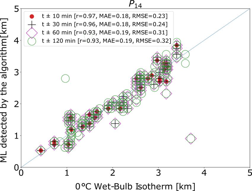
1 whole year of precipitation profiles, we concluded that the
∗ , Z ∗ and (1 − ρ ∗ ), i.e. P pro- Figure 13. Comparison of the MLA outputs based on the variable
profile that combines ZH DR HV 14 P10 for QVPs constructed from 9◦ elevation angle scans. Panel (a)
vides the best detection of the ML. The performance of the shows the detection of the melting layer for a stratiform event dis-
algorithm using this combination is shown in Fig. 12. played over a height versus time plot of ZH ; panel (b) shows the
Figure 12 shows that error and correlation coefficient de- performance for a convective event displayed over a height versus
crease as the time interval increase. Given that the errors time plot of ZDR .
are close to 250 m for short time windows, this combina-
tion proves to be accurate for the ML detection, making al-
lowance for the original resolution of the scans (600 m). A time window length. After several attempts with dif-
total of two examples of the outputs of the algorithm, using ferent time windows, we observed that the signatures
the profile P14 , are shown in Fig. 13 for the same stratiform of the melting layer are often easier to discern in pro-
and convective events as in Sect. 5.2. The combination P14 files related to stratiform events. However, for convec-
shows that the ML is correctly detected, and the delineation tive events, the main variables that detect the ML, e.g.
of the rain region is well executed. For the convective event ZDR or ρHV , are affected by the temporal averaging,
of Fig. 13b, the outputs of the algorithm are accurate for the blurring the melting layer signatures. Thus, we present
ML estimation, although some gaps are present due to the examples of instantaneous QVPs; however, we kept this
filtering of profiles in the first part of the algorithm. matter in mind for the MLA design.
ii. The spatial variation in the rain events is a limitation
6 Discussion of both VPs and QVPs. The former captures the storm
structure only directly above the radar location. More-
We constructed VPs and QVPs of polarimetric variables to
over, for the data sets used in this work, scans taken
explore precipitation events and their features. As shown in
at 90◦ elevation present limitations when reading data
Fig. 2, both types of profiles display differences influenced
on the first kilometre due to technical restrictions; this
by the scan elevation angle and the methods used to construct
situation restrains the observation of rainfall features at
the profiles. Regarding the latter, there are several points
relatively lower altitudes. On the other hand, the PPIs
worth discussing.
from where the QVPs are constructed may contain sec-
i. It is possible to generate time-averaged QVPs to smooth tors with non-homogeneous echoes, e.g. a combination
the effects related to local storm structures; the averag- of mixed precipitation is possible at ranges far from the
ing process over the radar domain, combined with tem- radar because the beam is considerably bigger. More-
poral averaging, reduces the signal noise, and it may over, at certain stages of the storm evolution, the radar
help to discard profiles with signatures not related to the echoes are insufficient to generate QVPs with clear sig-
melting layer. However, the duration of the rain events natures of the melting layer or even valid QVPs. This
and other factors raises a question about the correct horizontal heterogeneity introduces uncertainty into the
https://doi.org/10.5194/amt-14-2873-2021 Atmos. Meas. Tech., 14, 2873–2890, 2021You can also read