Linking zonal winds and gravity - II. Explaining the equatorially antisymmetric gravity moments of Jupiter
←
→
Page content transcription
If your browser does not render page correctly, please read the page content below
MNRAS 505, 3177–3191 (2021)                                                                                         https://doi.org/10.1093/mnras/stab1566
Advance Access publication 2021 June 2

Linking zonal winds and gravity – II. Explaining the equatorially
antisymmetric gravity moments of Jupiter
Wieland Dietrich ,1‹ Paula Wulff,1,2 Johannes Wicht                               1
                                                                                      and Ulrich R. Christensen1
1 Max   Planck Institute for Solar System Research, Justus-von-Liebig-Weg 3, D-37077 Göttingen, Germany
2 Georg  August University, Institute for Geophysics, Friedrich-Hund-Platz 1, D-37077 Göttingen, Germany

Accepted 2021 May 26. Received 2021 May 20; in original form 2021 February 26

                                                                                                                                                             Downloaded from https://academic.oup.com/mnras/article/505/3/3177/6291196 by guest on 10 October 2021
ABSTRACT
The recent gravity field measurements of Jupiter (Juno) and Saturn (Cassini) confirm the existence of deep zonal flows reaching
to a depth of 5 per cent and 15 per cent of the respective radius. Relating the zonal wind-induced density perturbations to the
gravity moments has become a major tool to characterize the interior dynamics of gas giants. Previous studies differ with respect
to the assumptions made on how the wind velocity relates to density anomalies, on the functional form of its decay with depth,
and on the continuity of antisymmetric winds across the equatorial plane. For the case of Jupiter, most of the suggested vertical
structures exhibit a rather smooth radial decay of the zonal wind, which seems at odds with the observed secular variation of the
magnetic field and the prevailing barotropy of the zonal winds. Moreover, the results relied on modifications of the surface zonal
flows, an artificial equatorial regularization or ignored the equatorial discontinuity altogether. We favour an alternative structure,
where the equatorially antisymmetric zonal wind in an equatorial latitude belt between ±21◦ remains so shallow that it does not
contribute to the gravity signal. The winds at higher latitudes suffice to convincingly explain the measured gravity moments.
Our results indicate that the winds are barotropic, i.e. constant along cylinders, in the outer 3000 km and decay rapidly below.
The preferred wind structure is 50 per cent deeper than previously thought, agrees with the measured odd gravity moments, is
compliant with the requirement of an adiabatic atmosphere and unbiased by the treatment of the equatorial discontinuity. We
discuss possible implications for the interpretation of the secular variation of Jupiter’s magnetic field.
Key words: gravitation – hydrodynamics – planets and satellites: gaseous planets.

                                                                                 profile are constrained by the gravity measurements (Kaspi et al.
1 I N T RO D U C T I O N
                                                                                 2010, 2013, 2018; Kong et al. 2018; Galanti et al. 2019). More
The spacecrafts Juno and Cassini delivered high-accuracy measure-                recently, constraints from Jupiter’s magnetic field (Duer, Galanti &
ments of the gravity potentials for Jupiter and Saturn (Iess et al. 2018;        Kaspi 2019) or it’s temporal evolution (Galanti & Kaspi 2020) have
Iess et al. 2019), which provide valuable constraints on the interior            also been used in addition to this. However, some studies found it
structure and dynamics of their atmospheres. For the first time, it has          necessary to partially modify the zonal flow compared to what is
been possible to resolve the tiny undulations in the gravity potential           observed at cloud level (Kong et al. 2018; Galanti & Kaspi 2020) in
induced by zonal winds (Guillot et al. 2018; Kaspi et al. 2018). This            order to match the modelled gravity anomalies to the observed ones.
has ended the long-standing debate on whether the zonal winds on                    Gravity moments of odd degree exclusively contain the impact of
Jupiter and Saturn are shallow weather phenomena or reach deeper                 equatorially antisymmetric zonal flows, since they are not obscured
into the planets’ convective envelopes. The gravity data suggest that            by the rotational deformation of the planet as opposed to their even
the winds extend down to 5 per cent and 15 per cent of Jupiter’s and             counterparts. The downward continuation of the antisymmetric zonal
Saturn’s radii, respectively (Kaspi et al. 2018, 2020; Galanti et al.            flows from each hemisphere yields opposite signs at the equatorial
2019). However, modelling the deep-reaching zonal mass fluxes on                 plane and hence introduces a problematic discontinuity or equatorial
a gas planet with all their complexity and relating them to anomalies            ‘step‘. This has been reported to potentially bias the results (Kong,
in the gravity field is a difficult, non-unique problem.                         Zhang & Schubert 2016). To circumvent this issue, several published
   The recent attempts of constraining the deep-reaching winds with              studies, such as Kaspi et al. (2018) and Galanti & Kaspi (2020) simply
gravity data are based on simple parametrizations of the vertical                ignore the contribution due to the equatorial step. Alternatively,
wind structure. The observed surface winds are thus continued                    Kong, Zhang & Schubert (2017) or Kong et al. (2018) suggested
downward along cylinders that are aligned with the rotation axis.                to smoothen the equatorial region artificially.
The resulting barotropic flow is then multiplied with a parametrized                Zonal winds induce perturbations in the gravity potential via pres-
radial profile to model the decay with depth. The parameters of this             sure perturbations that change the density distribution. The steady-
                                                                                 state, inviscid, non-magnetic Navier-Stokes (or Euler) equation, a
                                                                                 balance between pressure gradient; rotational forces; and gravity
   E-mail: dietrichw@mps.mpg.de                                                 forces; establishes the link between zonal flows and the induced

C The Author(s) 2021.

Published by Oxford University Press on behalf of Royal Astronomical Society. This is an Open Access article distributed under the terms of the Creative
Commons Attribution License (http://creativecommons.org/licenses/by/4.0/), which permits unrestricted reuse, distribution, and reproduction in any medium,
provided the original work is properly cited.
3178        W. Dietrich et al.
density perturbation. The gravity term has two contributions, one
due to the zonal-flow-induced density perturbation and a second due
to the dynamic gravity perturbation. If the latter, termed dynamic self
gravity (DSG) by Wicht et al. (2020), is ignored, the balance reduces
to the classic thermal wind equation (TWE) which can directly be
solved for the density perturbation and hence the gravity perturbation.
This approach has been commonly used for modelling the gravity
anomalies of Jupiter and Saturn and characterizing their deep interior
structure (Guillot et al. 2018; Kaspi et al. 2018; Galanti et al. 2019;
Iess et al. 2019). Several authors claim that the DSG term is indeed
negligible (Galanti, Kaspi & Tziperman 2017; Kaspi et al. 2018),
but this has been disputed by Zhang, Kong & Schubert (2015), Kong
et al. (2017), and Wicht et al. (2020).

                                                                                                                                                       Downloaded from https://academic.oup.com/mnras/article/505/3/3177/6291196 by guest on 10 October 2021
   Retaining the DSG-related term yields the so called thermo-
gravitational wind equation (TGWE), which is harder to handle
mathematically and numerically. Zhang et al. (2015) reformulate
the TGWE into an integro-differential equation for the density
perturbation. Their approach is restricted to polytropic interiors with   Figure 1. Various proposed radial decay functions alongside the expected
index unity. More recently, Wicht et al. (2020) show that the TGWE        amplitude of zonal flows that are compliant with the secular variation of
can be formulated as an inhomogeneous Helmholtz equation for              Jupiter’s magnetic field (Moore et al. 2019).
the gravity potential. The results show that the relative impact of
the DSG decreases with the spherical harmonic degree  of the             Jupiter’s observed magnetic field over the past decades, however, can
gravity perturbation. Being of order one for  = 2, it decreases to       be explained if the amplitude of the zonal wind at the depth of the
10 per cent at about  = 5 and becomes smaller than 1 per cent for       horizontal advection of the radial field, i.e. 4 per cent to 6 per cent of
> 25. However, the polytrope provides only a crude approximation          Jupiter’s radius, is as weak as cm s−1 compared to tens or hundreds of
of Jupiter’s interior. Here, we introduce a solution method for the       meters per second at the surface (Moore et al. 2019) (grey dots in the
TGWE that is based on formalism of Wicht et al. (2020) but can            figure). This result only holds under the assumption that the secular
also handle more realistic interior models that are reflected by a        variation at the surface indeed represents the horizontal advection of
radius-dependent DSG coefficient.                                         poloidal field lines at those radii. For shallower depth, the velocities
   The centrifugal force leads to a deformation of the planet and         can be faster than cm s−1 as long as the magnetic Reynolds number
thus renders the hydrostatic equilibrium state non-spherical. The         decrease with radius.
respective impact on the odd gravity moments has not been explored           More recently, Galanti & Kaspi (2020) showed that a combined
in great detail, though Kong et al. (2016) showed that it is smaller      gravito-magnetic analysis favoured a sharper radial profile with a
than 20 per cent for a model where the antisymmetric winds reach          2000 km deep barotropic part and 600 km decay region (red profile
down to the equatorial plane. For the even moments, the rotational        in Fig. 1). However, the authors found it necessary to modify the
flattening and the centrifugal force cause a 10 per cent variation        surface zonal flow profile in order to best match the gravity data. The
(Galanti et al. 2017). For simplicity, we ignore the effect of the        required flow modulations of up to 10 or 15 m s−1 seem to exceed the
rotational deformation on the odd gravity harmonics and focus             observational uncertainties of perhaps a few m s−1 (Tollefson et al.
on exploring the impact of the DSG term that has been studied             2017).
more.                                                                        In this study we revisit the key model assumptions and properties
   The discrepancy between existing studies of Jupiter’s odd gravity      on which the analyses of odd-degree gravity moments are based
moments is related to differences in the modelling assumptions.           and quantify their impact on the solutions. This includes justifying
Kaspi et al. (2018) explained the first four odd gravity moments          the fundamental equation, the problematic treatment of the equator,
of Jupiter by extending the observed zonal wind profile obtained          various surface zonal flows profiles and different models of Jupiter’s
during the perijove (Tollefson et al. 2017) along cylinders, inverting    interior.
the TWE equation, ignoring the discontinuity at the equatorial plane,
assuming a realistic Jupiter interior model (Guillot et al. 2003) and     2 T H E O RY
a relatively smooth radial decay (see Fig. 1, green). This has been
challenged by Kong et al. (2017), arguing that the TGWE should be         2.1 Governing equation
used. The subsequent application to Jupiter by Kong et al. (2018)
is based on a polytropic interior and the surface flow measurements       The gravity potential Ψ is directly related to the density distribution
from the Cassini mission (Porco et al. 2003). In order to carry this      ρ via the Poisson equation
out, the surface zonal flow was also modified by putting a cap on the     ∇ 2 Ψ = 4π Gρ,                                                        (1)
amplitude of the spike in the antisymmetric flow at β = 21◦ latitude,
and applied a second decay function to smooth out the discontinuity       where G is the gravitational constant. The general solution is
at the equatorial plane (orange profile).                                                   r θ
                                                                                                   ρ(r̃, θ̃) 2
   Both studies favour a rather smooth decay with depth in order          Ψ (r, θ ) = 4π G                  r̃ sin θ̃ dr̃ dθ̃                   (2)
to match the observed gravity signal, which implies quite significant                       0   0 |r − r̃|

flow amplitudes below 0.95 R. The radial decay profile of Kaspi et al.    and the associated gravity force is g = −∇Ψ . It is useful to separate
(2018) implies a remaining 10 per cent flow amplitude at 0.95 R,          the external gravity potential into a spherically symmetric part of a
whereas Kong et al. (2018) found more than half of the surface            non-rotating, solid body and a series of higher order terms originating
amplitude remaining at this depth. The weak secular variation of          from density perturbations and the rotational deformation of the

MNRAS 505, 3177–3191 (2021)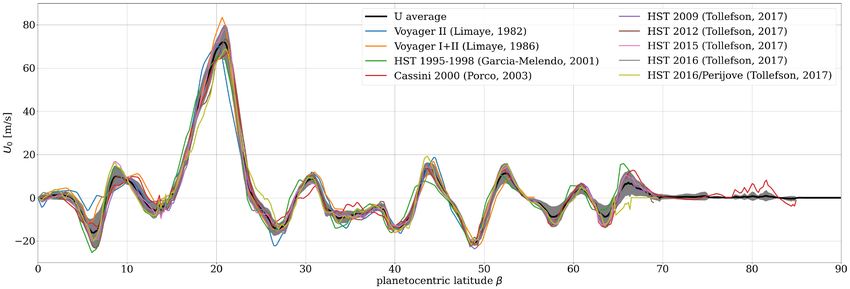
Zonal winds and gravity                3179
planet:                                                                                 vorticity equation yields the so called TGWE:

          GM                    ∞
                                                R                                       2 ∂z (ρUφ ) = φ̂ · (∇ × (ρ  ∇Ψ + ρ∇Ψ  ))                          (8)
Ψ =−         1−     J                                   P (cos θ ) ,            (3)
           r    =2
                                                r                                                         1 dΨ              1 dρ
                                                                                                    =−            ∂θ ρ  −         ∂θ Ψ  .              (9)
where R is the equatorial planetary radius, M the total mass, and P                                      r dr              r dr
are the Legendre polynomials of degree . The  = 1 contribution                        Replacing Ψ  by equation (2) and integrating over latitude leads to
vanishes because the origin of the coordinate system has been chosen                    the integro-differential equation solved by Zhang et al. (2015)
to coincide with the centre of gravity. The gravity moments J are                           θ
                                                                                                                           1 dΨ
given by:                                                                               2       ∂z (ρUφ (r, θ̃))dθ̃ = −            ρ
                                                                                              0                            r dr
                        R          π
                                                                                                     r θ 2
          2π                                                                                 1 dρ              r̃ ρ
J = −                                   ρ(r, θ ) P (cos θ) r +2 sin θ dθ dr.   (4)     −                             sin θ̃ dθ̃dr̃ + C(r).           (10)
          MR        0           0                                                           r dr 0 0 |r − r̃|

                                                                                                                                                                   Downloaded from https://academic.oup.com/mnras/article/505/3/3177/6291196 by guest on 10 October 2021

While the odd moments contain the signal of the equatorially                            While the integration function C(r) renders ρ mathematically non-
antisymmetric component of zonal flows, the even moments are                            unique, the gravity moments nevertheless remain unique (Kaspi et al.
dominated by the effects of the rotational deformation of the planet.                   2010; Zhang et al. 2015). The integration function C(r) would only
We therefore focus on the equatorially antisymmetric winds and the                      contribute to the spherical symmetric gravity harmonic which is
respective observed odd gravity moments J3 , J5 , J7 , and J9 . The                     determined by the total mass and therefore we can set C(r) to zero.
general relation between the zonal mass flux and a density anomaly                      Treating equation (7) is mathematically demanding and has so far
is expressed by the reduced Navier–Stokes equation, which describes                     only been solved for a simple interior model, i.e. a polytrope of index
the conservation of momentum for a steady, inviscid, non-magnetic,                      unity (Zhang et al. 2015; Kong et al. 2018).
inertia-less flow rotating around the ẑ-axis with a rotation rate . In                   A potential work-around was devised by Braginsky & Roberts
the co-rotating frame of reference this reads:                                          (1995) in the framework of classic geodynamo theory. It was shown
                                                                                        that the DSG term can be absorbed into the so-called effective
2 × (ρu) = −∇p + ρ∇Ψ + ρ ×  × r,                                               (5)   variables (density and pressure):

where the terms (from left to right) are the Coriolis force, the                        p e = p  + ρΨ                                                    (11)
pressure gradient, the gravity, and the centrifugal force. This leading                              μ
order force balance applies to the quasi-stationary zonal flows in                      ρe = ρ +        Ψ .                                           (12)
                                                                                                    4π G
the outer envelope where the electrical conductivity is so low that
                                                                                        The radial function μ is thereby characterized by the compressibility
the Lorentz force can be neglected. The centrifugal force in the
                                                                                        of the considered medium:
leading order force balance represents the rotational deformation
and renders the steady background state 2D and non-spherical (e.g.                        μ        ∂ρ      ρ     1 dρ
                                                                                               =ρ        = 2 =          ,                               (13)
Cao & Stevenson 2017). However, the rotational deformation itself is                    4π G       ∂p s    cs     g dr
rather insignificant for the antisymmetric problem (Kong et al. 2016)
                                                                                        where cs is the sound speed. For a polytropic perfect gas, this can be
and thus we ignore the centrifugal forces for now. A big advantage
                                                                                        further simplified,
of this approximation is that the fundamental equation can be written
                                                                                                           m+1
as a set of 1D PDEs, one for each spherical harmonic degree. Also,                       μ      m ρc m m−1
the eigenfunctions for the radial and latitudinal part of the Helmholtz                      =          ρ m ,                                              (14)
                                                                                        4π G   m + 1 pc
equation are known for the spherical problem.
   Pressure, density, and gravity are separated into a hydrostatic                      where m is the polytropic index, ρ c and pc are density and pressure
background that depends only on radius and a small perturbation,                        at the centre of the planet. They depend on the specific solution of
e.g. ρ = ρ(r) + ρ  (r, θ ). The first-order perturbation equation is then              the Lane–Emden equation. Moreover, for a polytropic index unity,
given by:                                                                               μ is a constant and amounts to π 2 /R2 .

                                                                                           The effective variables, pe and ρ e , are equal to p and ρ reduced by
2 × (ρu) = −∇p  + ρ  ∇Ψ + ρ∇Ψ  ,                                              (6)   the contribution of the local elevation or depression of the associated
                                                                                        equipotential surface thus capturing the effect of the DSG. Using
where the last two terms on the right-hand side are gravity force                       the effective variables and the definition of μ (equation 13), the
contributions due to a dynamic (i.e. flow-induced), density anomaly                     Navier–Stokes equation (equation 6) simplifies to:
(ρ  ∇Ψ ) and the DSG (ρ∇Ψ  ) term. In the classic thermal wind
approach (e.g. Kaspi et al. 2018), the DSG is neglected. The density                    2 × (ρu) = −∇p e + ρ e ∇Ψ .                                       (15)
anomaly can then simply be found from the TWE, which is the                             Taking the azimuthal component of the curl, integrating along
azimuthal component of the curl of equation (6):                                        colatitude θ and replacing ∇Ψ = g , then yields the effective density
               1                                                                        perturbation:
2 ∂z (ρUφ ) = − ∇Ψ ∂θ ρ  .                                                       (7)
               r                                                                                         r θ
                                                                                        ρ e (r, θ ) = 2      ∂z (ρUφ )dθ̃ := ρ U .                       (16)
An integration along latitude and division by the background gravity                                    g 0
yields the anomalous density field, which is subsequently used to                       Since this effective density disturbance formulates the zonal flow
calculate J by equation (4).                                                           impact, it has been called ρ U by Wicht et al. (2020) and we adopt

   Zhang et al. (2015) and Wicht et al. (2020) show that the DSG                        this name here. Note that this is not the true density disturbance ρ
                                                                                                                                                           U
term represents a first-order effect and, for example, changes the J3 -                 that could serve to calculate J via equation (4). In particular, ρ and

values by up to 30 per cent. Keeping the DSG term in the azimuthal                      ρ are related as defined by equation (12).

                                                                                                                            MNRAS 505, 3177–3191 (2021)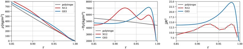
3180        W. Dietrich et al.
    Now we can find an equation for the gravity potential by replacing      yields

ρ with Ψ  using equation (1) in equation (9), integrating along                     2
latitude and making use of equation (16):                                   δT ≈        T   U.                                                 (21)
                                                                                      g

∇ Ψ + μΨ = 4π Gρ .
  2                     U
                                                                    (17)
                                                                            For Jupiter ≈ 1.76 · 10−4 s−1 and g ≈ 25 m s−2 . Then, in order
   This is a 2D, inhomogeneous PDE of second order, which                   to induce a vertical variation of the wind U = 10 m s−1 at a
describes the wind-induced anomalies in the gravity potential of a          temperature of T (r = 0.95R) = 4 · 103 K (Nettelmann et al. 2012),
gas planet (Wicht et al. 2020). The effective density perturbation ρ U      we find δT ≈ 0.5 K – an unrealistically high value considering
derived from equation (16) acts as the source term for this Helmholtz-      that the temperature fluctuations associated with convective motions
like equation. Only when μ = const does this equation become an             are on the order of 10−4 K (e.g. Jones 2007). These estimates are
inhomogeneous Helmholtz equation and can be solved in a semi-               applicable to the convective part of the atmosphere, i.e. below
analytical way (Wicht et al. 2020). In the more general case where μ        p = 1 bar.
depends on the radius, we refer to the numerical methods discussed             In conclusion, whenever convection restricts the degree of non-

                                                                                                                                                       Downloaded from https://academic.oup.com/mnras/article/505/3/3177/6291196 by guest on 10 October 2021
in Section 4.                                                               adiabaticity, the zonal flows Uφ (and not the mass flux) are cylindri-
   It is important to note that the second order differential equation      cally invariant. This analysis also rules out any vertical wind profile
(equation 17) and the integro-differential form of the TGWE (equa-          that is gradually decaying throughout the convective zone (Kaspi
tion 10) describe the same physical problem. The main difference            et al. 2018; Kong et al. 2018). This suggests that a substantially
is that equation (17) solves for Ψ  , while equation (10) solves for       subadiabatic zone, e.g. a stable stratified layer might be needed to

the density anomaly ρ . Equation (17) not only directly provides the        generate a sufficient degree of baroclinicity and ultimately damp the
gravity potential we are interested in, but is also much easier to solve.   winds (Christensen, Wicht & Dietrich 2020).

                                                                            3 PA R A M E T R I Z I N G T H E DY N A M I C D E N S I T Y
2.2 Cylindrical invariance of the zonal winds
                                                                            P E RT U R BAT I O N
The effective variables can be further exploited to show that the
                                                                            The dynamic density perturbation (equation 16) is governed by the
flow (Uφ ) and not the mass flux (ρUφ ) is barotropic and should
                                                                            assumed interior structure of the planet via the background density
be initially extended along cylinders. To emphasize under which
                                                                            and gravity, ρ and g, respectively, and the z-gradient of the zonal mass
conditions barotropic winds can be modulated along the rotation
                                                                            flux. Theoretical considerations and numerical simulations suggest
axis, we express the density as a function of pressure and entropy:
                                                                            a cylindrically invariant, i.e. barotropic zonal flow structure for the
s   cv p e   ρe   cv p   ρ                                               fast rotation and low viscosity gas planets (e.g. Taylor 1917; Dietrich
   =        −    =        − .                                       (18)
cp   cp p     ρ    cp p    ρ                                                & Jones 2018; Gastine & Wicht 2021). This means that the flow
                                                                            depends only on the distance s = rsin θ to the rotation axis, where
Dividing the Navier–Stokes equation (equation 15) by the back-
                                                                            θ is the colatitude. We could then simply downward continue the
ground density and defining a reduced pressure p  = p e /ρ, equa-
                                                                            surface zonal flow U0 along cylinders.
tion (15) yields:
                                                                               However, the gravity measurements and the secular variation of the
          1          ρe                                                     Jupiter’s magnetic field show that the wind speed must significantly
2 × u = − ∇p e + ∇Ψ
          ρ          ρ                                                      decrease with depth and should be confined to outer 5 per cent of
             e
              p         pe      cV p e   s                                 the planetary radius (Kaspi et al. 2018; Moore et al. 2019; Galanti
       = −∇          − 2 ∇ρ +          −      ∇Ψ                            & Kaspi 2020). This decrease is commonly parametrized with an
               ρ        ρ       cp p     cp
                                                                          additional radial decay function Qr ,
                  s         cV ρ 2            pe
       = −∇ p  − ∇Ψ +              ∇Ψ − ∇ρ                                 Uφ (r, θ ) = Qr (r) Uo (s)                                         (22)
                  cp         cp p              ρ2

                 s                                                          with Qr (R) = 1. The cause for the deviation from barotropy remains
        −∇p  − ∇Ψ .                                               (19)
                 cp                                                         unspecified. Electromagnetic effects have been alluded to. Buoyancy
                                                                            forces arising in a stably stratified region with the assistance of
Note, the term in the brackets scales with the non-adiabaticity of the
                                                                            Lorentz forces are a promising mechanism (Christensen et al. 2020;
background state and hence can safely be neglected for a vigorously
                                                                            Gastine & Wicht 2021). We start with discussing the interior state,
convecting atmosphere like Jupiter’s. This equation highlights that
                                                                            then the different models of the surface zonal profile and finally the
the winds Uφ and not the mass fluxes are cylindrically invariant. Only
                                                                            calculation of the dynamic density source ρ U .
if there are sizeable latitudinal gradients in the zonally averaged
entropy, deviations from the cylindrical invariance are possible
if we restrict the consideration to regions of negligible electrical        3.1 Interior state
conductivity. The associated temperature fluctuations required to
drive the zonal wind out of its cylindrical invariance can be estimated     The source term (equation 16) and the DSG coefficient, μ, depend
by azimuthal component of the curl of equation (19):                        on the background density and gravity profile, ρ and g, respectively.
                                                                            We explore their influence via the chosen interior state model by
                g
2 ∂z Uφ = −         ∂θ s  ,                                       (20)     comparing three commonly used models.
               cp r                                                           A simple model for Jupiter’s interior is a polytropic ideal gas
where dΨ /dr = g has been used. Assuming that the vertical and              of index unity that provides a decent description of the pressure
latitudinal derivative can be approximated with the same length scale       dependence on the density (Hubbard 1999), but not of the (p −
(e.g. close to the equator), thus ∂ z Uφ ≈ U/δ and 1/r ∂θ s  ≈ δs/δ.       T)-curve. The background density is then:
Furthermore, the entropy fluctuations can be (to first order) approx-                  sin χ            πr
                                                                            ρ(r) = ρ c       , with χ =    ,                                (23)
imated by temperature fluctuations, thus δs ≈ cp /T δT . This then                       χ              R

MNRAS 505, 3177–3191 (2021)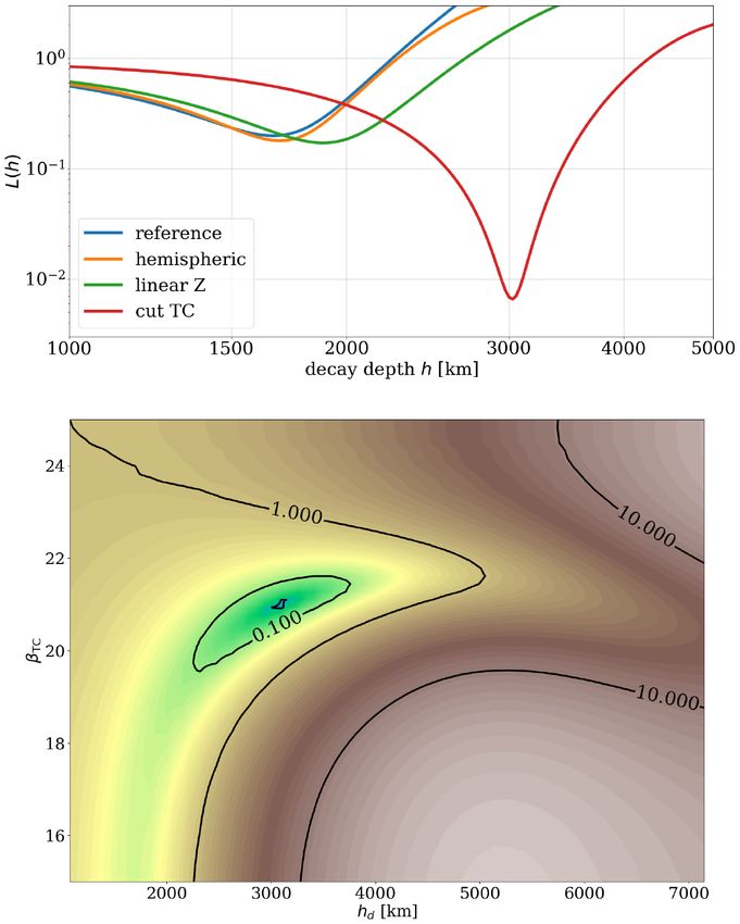
Zonal winds and gravity                     3181

Figure 2. Jupiter’s interior density ρ (left), radial gradient ∂r ρ and μ = ∂r ρ/g in the outer 15 per cent of radius from two Jupiter interior models in comparison
to a polytropic perfect gas with index unity (grey). The interior models based on three-layer internal structure are adopted from Guillot et al. (2003; blue) and
Nettelmann et al. (2012; red). The dots on the curve are based in ab initio calculations of the sound speed (cs2 ∝ μ) by French et al. (2012).

                                                                                                                                                                       Downloaded from https://academic.oup.com/mnras/article/505/3/3177/6291196 by guest on 10 October 2021
where ρ c is the central density. The associated background gravity                  measurements of the wind profile stem from late 2000 (red; Porco
is given by                                                                          et al. 2003). Later, various different HST-based profiles were obtained
                    χ cos χ − sin χ                                                  between 2009 and 206, during the perijove nine of the Juno space
g(r) = −4RGρ c                                                           (24)        craft (Tollefson et al. 2017). Kaspi et al. (2018) and Galanti & Kaspi
                          χ2
                                                                                     (2020) use this most recent flow profile for their gravity data analysis,
and is hence directly proportional to the radial density gradient as                 while Kong et al. (2018) prefer the model based on Cassini images
discussed in Zhang et al. (2015). This proportionality (g∝dρ/dr) is                  from late 2000 to early 2001 presented in Porco et al. (2003).
an exclusive property of a polytrope with index unity and implies a                     All flow models show the same principle structure but also differ
constant μ = π 2 /R2 . This has been exploited by Zhang et al. (2015)                in some details. The equatorially antisymmetric flow contribution
and Wicht et al. (2020) to solve the TGWE. The grey profiles in Fig. 2               shown in Fig. 3 is clearly dominated by the prograde jet which starts
illustrate the density, its radial gradient, and μ for the polytrope of              at a latitude around β = 17◦ and extends to about β = 23◦ . The
index m = 1.                                                                         amplitude of this jet varies between 65 m s−1 and 75 m s−1 for the
   The first analysis of the Juno gravity data by Kaspi et al. (2018)                different models.
was based on a Jupiter interior model by Guillot et al. (1994, 2003).                   Tollefson et al. (2017) conclude that the variations exceed the
This model is henceforth named ‘G03‘ and assumes a three layer                       model errors, at least for some epochs and at some latitudes. Their
structure with a helium-depleted, molecular outer hydrogen layer, a                  Lomb–Scargle periodogram analysis reveals dominant variation
helium-enriched metallic inner hydrogen layer and a central dense                    periods of about 7 and 14 yr. Since the latter is close enough to
core. Fig. 2 shows the density, density gradient, and μ for a setup with             Jupiter’s orbital period of 11.9yr and the former to the respective
interpolated hydrogen EOS, a 1-bar temperature of 165 K, a core of                   first overtone, the variations may represent seasonal cycles. These
4.2 earth masses, and heavy element abundance of 33 earth masses                     variation are unlikely to penetrate deeper into Jupiter’s atmosphere
(Guillot et al. 2003). In comparison to the rather simple polytropic                 and therefore play no role for the gravity signal. The arithmetic mean
model (grey), the densities are substantially higher for r < 0.975 R                 profile, shown as a black line in Fig. 3, should represent the deeper
and slightly lower above this radius. Thus the density gradient shows                flows more faithfully than a single model. The standard deviation
a pronounced maximum around r = 0.97 R (Fig. 2, middle panel).                       is highlighted as a function of latitude (±1σ , grey band), whereas
The DSG coefficient (μ) increases with radius and reaches a 2.5 times                its latitudinal mean is somewhat smaller than 3 m s−1 . Note that
larger value than for the polytrope.                                                 the flow modifications applied by Galanti & Kaspi (2020), which
   Alternatively, we use the more recent calculations from Nettel-                   were required to explain the gravity moments reach 10 or 15 m s−1
mann et al. (2012) based on the updated H-REOS2 model (‘N12‘).                       clearly exceeding the statistical fluctuations. However, the average
The DSG coefficient is related to the sound speed (equation 13),                     only covers a period of about 36 yr, or about three times the seasonal
which was calculated for the same Jupiter model by French et al.                     cycle, with a small number of ‘snapshots‘. Smaller deviations from
(2012). For this model (termed J11-8a), the depth of the molecular-                  the time average are thus certainly conceivable. We mostly rely on
metallic phase transition is at p = 8 Mbar, whereas in G03 model                     the mean wind profile but also explore the impact of using specific
this happens at shallower 2 Mbar. As shown in the left-hand panel of                 snapshots on the gravity signal in Section 5.6.
Fig. 2 the N12 model yields the highest density for r < 0.92 R and
falls between the G03 model and the polytrope at larger radii. The
density gradient and hence μ show two distinct maxima with smaller                   3.3 Treatment of the equatorial discontinuity
amplitude than the G03 model.                                                        An obvious problem arises with the equatorially antisymmetric
                                                                                     contributions to the dynamic density source. Cylindrically downward
3.2 Jupiter’s surface zonal flow                                                     continuing the surface flow in each hemisphere separately yields a
                                                                                     discontinuity, or step, at the equatorial plane. It can be large in case
The surface flow of Jupiter is deduced from tracking cloud features,                 the continuation of the surface flow hits the equatorial plane at a
either with the Hubble Space Telescope (HST) or from space crafts.                   radius where Qr is significantly larger than zero. This equatorial step
Fig. 3 displays several zonal flow measurements that have been                       seems unphysical but can easily be dealt with mathematically.
obtained over the last decades. The oldest illustrated flows (blue                      Using the product ansatz (equation 22) in equation (16), we can
and yellow) are based on observations by Voyager I and II (Limaye                    separate the dynamic density perturbation into two contributions:
et al. 1982; Limaye 1986) and represent the flow in 1979. HST                                                     θ                      θ
monitored the wind structure several times between 1995 and 1998                              2 r ∂                                          ∂Uo
                                                                                     ρU = −              (ρQr )      Uo cos θ̂dθ̂ + ρQr           dθ̂ . (25)
(green profile; Garcı́a-Melendo & Sánchez-Lavega 2001). Cassini                                g    ∂r           0                        0  ∂z

                                                                                                                             MNRAS 505, 3177–3191 (2021)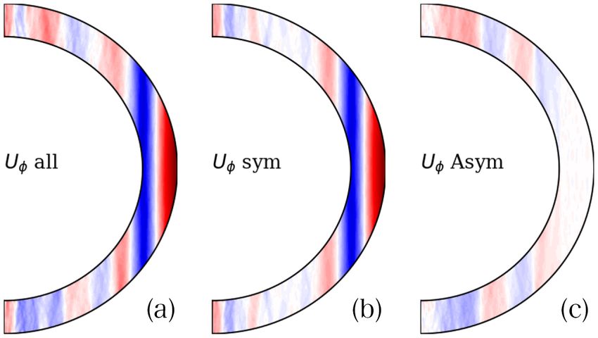
3182         W. Dietrich et al.

                                                                                                                                                                  Downloaded from https://academic.oup.com/mnras/article/505/3/3177/6291196 by guest on 10 October 2021
Figure 3. Comparison of different zonal flow models for Jupiter observed either by HST or in situ by space crafts. Shown is the equatorial antisymmetric flow
part relevant for the odd gravity moments. The models are from the Voyager mission Limaye et al. (1982, 1986), Cassini Porco et al. (2003), and various Hubble
Space Telescope (HST) campaigns (Garcı́a-Melendo & Sánchez-Lavega 2001; Tollefson et al. 2017). The black profile and the grey band are the arithmetic
mean profile and the standard deviation.

The second integral contributes only at the equator where the z-
derivative yields a delta-peak. This can be integrated analytically:
                           θ
         2 r ∂                                ρQr
ρU = −             (ρQr )     Uo cos θ̂ dθ̂ +     H (θ − π/2) U ,
           g ∂r            0                   r
                                                                  (26)
where H is the Heaviside step function and U = 2Uo (θ → π /2).
  As we will show below, the equatorial step can yield an important
contribution to the gravity signal which is problematic. Kaspi et al.
(2018) therefore ignore the respective term in an approach they call
‘hemispheric‘. They calculate ρ U in each hemisphere but dismiss the
contribution at (or very close to) the equator, which is equivalent to
evaluating
                          θ                                                      Figure 4. Zonal flow from the full 3D numerical model (a) separated into
         2 r ∂                                                                    the equatorial symmetric part (b) and the antisymmetric (c) part. The contour
ρU = −            (ρQr )     Uo cos θ̂ dθ̂ .                     (27)             levels are identical amongst the panels.
          g ∂r            0

This approach seems to offer a simple fix but is also inconsistent
since the step is an integral part of the chosen flow model. In the               Gastine & Wicht (2012)), a broad equatorial prograde jet develops,
model of Galanti & Kaspi (2020), the flows are sufficiently shallow               flanked by a deep retrograde jet adjacent to the tangent cylinder
and drop quickly enough with depth such that ignoring the equatorial              (TC). The TC is a virtual cylinder touching the inner boundary at
discontinuity does not affect the conclusion substantially.                       the equator and forms an important dynamical boundary in rotating
   Alternatively, Kong et al. (2018) use an additional linear z-                  convection. At higher latitudes, i.e. within the TC, alternating jets
dependence of Uo , such that the vertical gradient at the equator                 develop in both hemispheres. These winds show minimal variations
is regular and smooth. Their zonal flow model is thus given by                    in the direction of the rotation axis. Simulations at even more realistic
                  |z|                                                             parameters yield solutions with higher degrees of barotropy but are
U (r, θ ) = Qr         Uo (s) ,                                        (28)
                 |zo |                                                            also more numerically demanding (Heimpel, Gastine & Wicht 2016;
                                                                                  Gastine & Wicht 2021).
where |zo | = (R2 − s2 )1/2 is the local distance from the equatorial                Panels (b and c) of Fig. 4 show that the equatorially symmetric flow
plane to the surface. The equatorial step and the linear z-dependence             is dominant outside the TC and that the equatorially antisymmetric
are the steepest and smoothest end member, respectively, of the                   zonal flow is much weaker outside than inside the TC. Outside of
possible functions that reconcile the northern and southern zonal                 the TC, equatorially antisymmetric flows are at odds with barotropy.
flows.                                                                            Inside the TC, however, antisymmetric contributions can be, and
   Here, we introduce a novel approach guided by the physical                     indeed are, highly barotropic. The same dynamical reasons that
principles of atmospheric dynamics. The generation of deep-reaching               enforce barotropy (dominant Coriolis force and small viscosity) also
zonal flows powered by the statistical correlations of the convective             allow for only weak equatorially antisymmetric flows outside the
flows (Reynolds stresses) are best captured in numerical simulations              TC.
(Heimpel, Aurnou & Wicht 2005; Christensen 2002; Dietrich &                          To account for this physical property of zonal flow in rotating
Jones 2018; Gastine & Wicht 2021). Fig. 4 illustrates the zonal flow              spherical shells, we multiply the antisymmetric surface flow with an
in a typical simulation of convection in a fast rotating spherical shell          additional attenuation function Qs that reduces the amplitude outside
with an aspect ratio of ri /R = 0.8 using the MAGIC code (Wicht 2002;             of the latitude β TC , i.e. where the TC touches the outer boundary:
Gastine & Wicht 2012; Schaeffer 2013). For the chosen parameters
(E = 3 · 10−5 , Pr = 0.25, Ra = 7 · 107 , Nρ = 2.3, definition as in              Uo = Uo (s) Qs ,                                                       (29)

MNRAS 505, 3177–3191 (2021)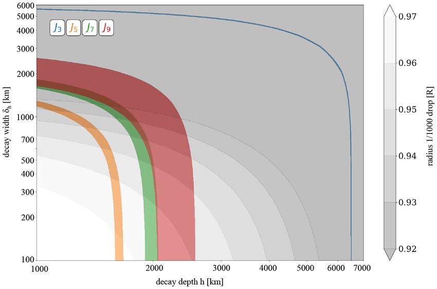
Zonal winds and gravity 3183
with For δh = 200 and h = 2000 km, the profile would be virtually
identical to the one suggested by Galanti & Kaspi (2020). However,
1 β − βTC β + βTC
Qs = tanh − tanh + 1. (30) our analysis favours a substantially deeper flow with h = 3000 and
2 δβ δβ
δh = 500 km. Fig. 1 shows the respective decay function in blue.
A second parameter which is introduced here is the width of the
latitudinal cutoff, δ β . Both functions, Qs (β TC , δ β ) and Qr (h, δ h ),
define an individual TC and hence should be consistent. More details 4 NUMERICAL METHOD
on selecting the best parameter combination for β TC , δ β , h, and δ h are
The semi-analytical method for solving the TGWE (equation 17)
discussed in Section 5. When β TC is sufficiently large and the radial
developed by Wicht et al. (2020) is restricted to the case of a constant
decay function drops rapidly below a certain depth, the resulting
μ. However, as shown in Fig. 2, μ(r) varies strongly and reaches
flow splits into an independent northern and southern part. Then
much higher values than π 2 /R2 , particularly in the outer 10 per cent
the equatorial step contribution is identical to zero. The underlying
of Jupiter’s radius where the flow-induced gravity moments originate
assumption is that part of the observed zonal flow at cloud level,
from. We have therefore developed a numerical method that can also
in particular its antisymmetric parts at low latitude, are shallow. We
Downloaded from https://academic.oup.com/mnras/article/505/3/3177/6291196 by guest on 10 October 2021
handle radial variations in μ.
term cases that apply such an attenuation of antisymmetric surface
We first formulate the dynamic density source ρ U (r, θ ) via
flows at low latitudes ‘TC-models’.
equation (26) in spatial space by choosing a radial decay function
Qr , an interior state model setting ρ, g, and μ, and a surface zonal
3.4 Radial decay function flow profile Uo that is cylindrically downward continued.
We then expand the latitudinal dependence of the gravity potential
The different forms of the radial decay function Q(r) that have been perturbation Ψ and the dynamic density ρ U in Legendre polynomi-
suggested to explain the gravity observations are illustrated in Fig. 1. als, e.g. for the former this is given by
Kaspi et al. (2018) use a combination of an exponential decay and a
hyperbolic tangent:
L
Ψ (r, θ ) = Ψ (r)P (cos θ), (35)
r − (R − h) h
Qr (α, h, δh ) = α tanh +1 tanh +1 =0
δh δh
with
r −R
+ (1 − α) exp . (31) π
h Ψ (r) = Ψ (r, θ )P (cos θ) sin θdθ. (36)
0
Here α is the weight of the hyperbolic tangent contribution, h the
Since the background state, and hence μ, are only a function of
decay depth, and δ h the decay width. For explaining the gravity
radius, the TGWE (equation 17) decouples for each degree , and
observations, Kaspi et al. (2018) propose a large α = 0.92, a relatively
we are then left with a set of radial ODEs, one for each spherical
large δh = 1570 km, and a depth of h = 1803 km. This results in a
harmonic degree :
smoothly decaying radial profile (green) illustrated in Fig. 1.
Kong et al. (2018), on the other hand, used an inverse Gauss 2 ( + 1)
profile ∂r2 + ∂r − + μ Ψ (r) = 4π GρU (r). (37)
r r2
1 H2 At the outer boundary, the potential must match to the solution
Qr (h, H ) = exp 1− 2 , (32)
h H − (1 − r)2 of a source free region, i.e. ∇ 2 Ψpot = 0, with the characteristic
for r > H, and Qr = 0.0 for r ≤ H. Kong et al. (2018) report that radial dependence r−( + 1) . This leads to the mixed outer boundary
the observations are best matched with a combination of H = 10 484 condition:
and δh = 15 377 km. Fig. 1 shows that the respective profile (orange) R
Ψ (R) = − ∂r Ψ (R), (38)
decays also rather smoothly. +1
Both the solution suggested by Kaspi et al. (2018) and by Kong
and Ψ (0) = 0 at the inner boundary.
et al. (2018) are not compatible with the magnetic observations
Our numerical method relies on an expansion in the modified
(Moore et al. 2019). Furthermore, vigorous convection provides an
spherical Bessel functions introduced by Wicht et al. (2020). These
almost adiabatic environment and hence the decay functions should
are radial eigenfunctions of the homogeneous Helmholtz equation.
be rather flat with a sharp drop at greater depth (see also Section 2.2).
For each spherical harmonic degree , we construct a set of N
Realizing this, Galanti & Kaspi (2020) proposed a steeper decaying
normalized orthogonal functions jn (kn r). The radial scales, kn ,
alternative with a hyperbolic tangent outer, and an exponential inner
are determined by finding the first N radii (starting at the origin),
branch:
⎧ at which jn (kn r) fulfils the boundary condition (equation 38). The
⎨α tanh r−rT / tanh h + 1 − α for r ≥ rT radial functions Ψ (r) are expanded in jn
:
δh δh
Qr = (33)
⎩(1 − α) exp r−r T for r < rT .
N
Ψ (r) =
δh
Ψn jn (kn r), (39)
They suggest α = 0.45, h = 2002 km, rT /R = 0.972, and δh = n=1
δh = 204 km in conjunction with an optimized surface flow profile where the expansion coefficients Ψn
are given by
to explain the gravity observations. The radial profile drops almost
R
faster than the magnetic constraints require (see fig.1).
Ψn = Ψ (r) jn
(kn r) r 2 dr. (40)
We adopt the pure hyperbolic tangent profile: 0
r − (R − h) h Since the modified spherical Bessel functions are eigenfunctions of
Qr (h, δh ) = tanh +1 tanh + 1 . (34)
δh δh the Laplace operator, equation (37) transforms into a set of linear
MNRAS 505, 3177–3191 (2021)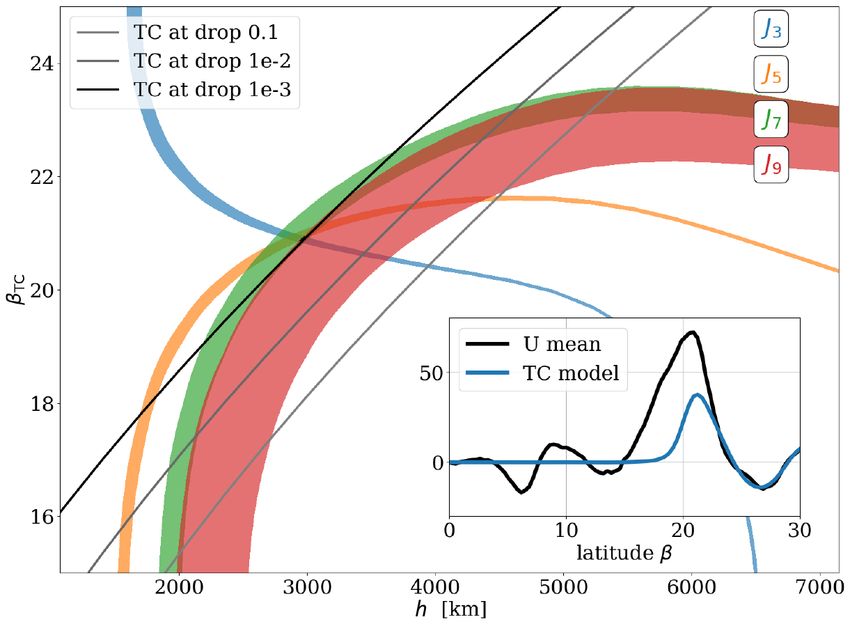
3184 W. Dietrich et al.
algebraic equations for the expansion coefficients Ψn :
N
μ(r) − kn
2
Ψn jn (kr) = 4π GρU (r). (41)
n=1
Equation (41) defines a coupled set of algebraic equations and solved
by using a matrix formalism. The source term, ρU , on the RHS is
discretized along N radial grid points, ri . The solution of the matrix
equation, Ψn , contains the Bessel function expansion coefficients of
the gravity field perturbation. We thus introduce a square matrix H
defined by
Hn i = μ(ri ) − kn 2
jn (kn ri ), (42)
where n, i ∈ [1, N]. Then the TGWE with radially varying DSG
Downloaded from https://academic.oup.com/mnras/article/505/3/3177/6291196 by guest on 10 October 2021
coefficient can be written in the symbolic matrix form
H Ψ n = 4π Gρ U , (43)
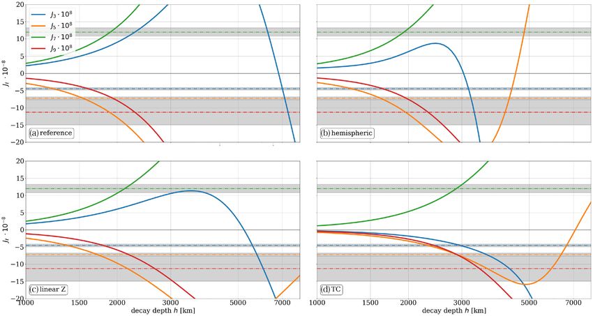
Figure 5. Trade-off between decay depth h and decay width δ h . The
where ρ U represents the source vector per degree along all radial coloured contours indicate combinations, where individual gravity moments
grid points and Ψ n is the solution vector containing the expansion are compatible within the uncertainties with the measurements (J3 blue, J5
coefficients. The matrix equation is solved via LU factorization. For orange, J7 green, and J9 red), while the grey shaded areas indicate a flow
dealiasing, we thus ignore the highest 10 per cent of the Bessel decay by three orders of magnitude at various depths as required by Jupiter’s
secular variation (Moore et al. 2019).
coefficients. We use an equidistant radial mesh with up to N = 1024
grid points, Gauss-Legendre points along latitude (Nθ = 4096) for
an accurate Legendre expansion (equation 36) and solve for the first
Semitransparent, coloured, regions indicate the parameter com-
four odd spherical harmonic degrees ( = 3, 5, 7, 9).
binations where the respective gravity harmonic stays within 3σ of
Having obtained the solution Ψn in Bessel space, equation (39)
the observations (Durante et al. 2020). There is a trade-off between
yields the radial representation Ψ . The gravity moments are then
both parameters since increasing either boosts the impact of deeper
simply given by
regions. Unfortunately, there is no parameter combination where all
R 2 + 1 stripes overlap, i.e. no combination of h and δ h that would explain all
J = Ψ (R), (44)
GM 2 four odd harmonics with one single decay function. Gravity harmonic
If required, the density perturbation can be calculated by solving J3 seems to be particularly problematic as it always maintains some
∇ 2 Ψ = 4π Gρ . distance from the other three, since to match it requires particularly
To test our method, we compare the solution for constant μ with deep sources.
results using the semi-analytical method introduced by Wicht et al. The grey background contours show at which radius the radial
(2020). To verify our method with radius-dependent μ, we solve decay function Qr would have decayed by three orders of magnitude.
equation (37) with an independent solver based on the shooting The SV constraint by Moore et al. (2019) suggests that this should
method. This is a standard tool for solving initial value problems and happen somewhere between r = 0.93 R and r = 0.96 R. Modelling
can readily be applied here, making use of a variable transformation the observed J3 always requires deeper sources that are incompatible
to account for the asymptotic behaviour at the origin when applying with this constraint. For the smooth decay functions suggested by
this method. Kaspi et al. (2018) or Kong et al. (2018), the three orders of magnitude
drop lies far below r = 0.90 R (see also Fig. 1).
Numerical simulations and theoretical consideration suggest that
5 M O D E L L I N G T H E G R AV I T Y
the flow remains barotropic until a stably stratified layer, Lorentz
P E RT U R BAT I O N S
forces or a combination of both, drastically quench the amplitude
We start by exploring the challenges of modelling the odd gravity over a few hundred kilometres (Christensen et al. 2020; Wicht &
perturbations for a reference model that combines the interior Gastine 2020). We therefore restrict our analysis to δ h = 500 km in
model by Guillot et al. (2003) with the average flow introduced the following, a value that represents the scale height of the electrical
in Section 3.2 and employs the TGWE method (equations 37 or 41). conductivity in the outer atmosphere of Jupiter quite well (French
The required dynamic density source is calculated via equation (26), et al. 2012; Wicht et al. 2019) and will be further validated from the
where we assume a hemispherically barotropic flow while keeping results of the TC model (see Section 5.2).
the equatorial step and applying the hyperbolic tangent radial decay Fig. 6 illustrates how the gravity harmonics change when varying h
profile for Qr in accordance with equation (34). while keeping δh = 500 km fixed. For the reference model (Fig. 6a),
the harmonics J5 , J7 , and J9 all agree with the respective observations
for h values between 1500 and 2300 km. However, J3 requires much
5.1 Reference model and equatorial treatment
deeper flows with h ≈ 6500 km. Table 1 gives the values for h and
Fig. 5 shows an attempt to model the observed gravity harmonics the respective uncertainties for all considered models. We use the
by varying the two parameters in Qr , the decay depth h, and the spherical harmonic degree as an index to denote the different values
decay width δ h . A latitude-dependent attenuation in the form of of h required to explain the different observations. For a successful
equations (28 or 29) is not applied at this point. To assess the quality model, all four h-values must agree within the errors. This is clearly
of the modelled gravity moments, we compare them individually not the case for our reference model. Only for degree = 7 and =
for each degree to the observations rather than minimizing an - 9, the decay depths match within the uncertainties at h ≈ 2000 km.
independent, global cost-function (Kaspi et al. 2018). For reasonable values of h between 2000 and 4000 km, the modelled
MNRAS 505, 3177–3191 (2021)
Zonal winds and gravity 3185
Downloaded from https://academic.oup.com/mnras/article/505/3/3177/6291196 by guest on 10 October 2021
Figure 6. Odd gravity moments (degree = 3, 5, 7, 9 in blue, orange, green, and red) as function of the decay depth alongside the measurements (horizontal
lines) and 3σ uncertainties (Durante et al. 2020). Panel (a) represents the reference model using the full surface flow, a barotropic downward continuation and
including the equatorial step, whereas in (b), the equatorial step is ignored. In (c), the additional linear z-decay is applied, and (d) utilizes a zero flow outside
TC. More details in the text or in Table 1.
Table 1. List of the models with the different treatment of the equator, different solvers, interior models, and surface flows. Further given is the decay depth h
at which the modelled gravity moment agrees with the observations (Durante et al. 2020).
Name Equator Solver Interior Surface flow h3 (km) h5 (km) h7 (km) h9 (km)
Reference Full TGWE G03 Mean 6541+14
−13 1556+43
−40 1923+85
−81 2270+248
−302
Hemispheric Hemispheric TGWE G03 Mean 3179+7
−7 1597+35
−34 1932+82
−79 2280+263
−304
Linear z Linear z TGWE G03 Mean 5127+23
−25 1735+42
−44 2143+106
−102 2614+369
−404
TC TC TGWE G03 TC cut 2950+94
−98 2895+81
−83 2883+135
−129 3433+404
−471
TWE Full TWE G03 Mean 5670+25
−27 1713+44
−47 1993+78
−80 2314+260
−311
cTGWE Full cTGWE G03∗ Mean 6190+18
−18 1630+41
−41 1956+87
−82 2294+250
−307
Perijove Full TGWE G03 HST, perijove 6480+13
−13 1541+42
−39 2033+88
−83 2339+254
−306
Cassini Full TGWE G03 Cassini 7005+15
−15 1539+43
−40 1901+85
−81 2289+249
−311
Cap Full TGWE G03 Capped Cassini 6263+15
−15 1708+45
−45 2041+91
−87 2434+276
−331
Poly Full TGWE polytropic Mean 6213+23
−23 1637+52
−54 2043+107
−102 2465+306
−370
N12 Full TGWE N12 Mean 6215+18
−18 1426+47
−48 1791+99
−92 2219+279
−345
gravity moment J3 is of the wrong sign, whereas J5 is much larger and find a reasonably good agreement of the decay depths across the
than the observed value in that range of h. degrees.
Panel (b) in Fig. 6 illustrates that the situation improves when we Panel (c) of Fig. 6 shows the results when using the additional
follow the approach by Kaspi et al. (2018) and ignore the contribution linear z-dependence suggested by Kong et al. (2018). This leads to
due to the equatorial step in equation (26). While the values of shallower winds closer to the equator, a smooth vertical gradient and
h5 , h7 , and h9 remain nearly unchanged, h3 decreases by half to thus no equatorial step. Again, h3 decreases significantly, but not as
about 3200 km (see also Table 1). This shows the large impact of much as for the model that ignores the equatorial step. The other
the equatorial discontinuity, in particular on degree = 3. If in harmonics are somewhat more affected, such that all h increase by
addition to this we assume the smoothly decaying radial function Qr roughly 10 per cent with respect to the reference model (Table 1).
suggested by Kaspi et al. (2018), ignore the DSG term and utilize the Though this additional modification of the vertical flow structure
perijove surface flow model, we can largely reproduce their results avoids the equatorial discontinuity, it is hard to justify physically.
MNRAS 505, 3177–3191 (2021)
3186         W. Dietrich et al.
                                                                                  i.e. where the associated drop-off equals Qr = 10−1 (light grey), Qr =
                                                                                  10−2 (dark grey), or QR = 10−3 (black). Mathematically, the surface
                                                                                  latitude β Q based on a specific Qr -value is given by
                                                                                         180◦        r
                                                                                               cos−1
                                                                                                        Q
                                                                                  βQ =                                                              (45)
                                                                                           π            R
                                                                                  where

                                                                                                              h
                                                                                  rQ = δh tanh−1 Qr     tanh     +1 −1 +R+h                          (46)
                                                                                                              δh
                                                                                  is the inverse of the decay function. β Q is now calculated for each
                                                                                  value for each decay depth h and the three different values of Qr .
                                                                                     Interestingly, the black line exactly hits the intersection point of
                                                                                  the coloured isocontours. This means that the TC defined by reducing

                                                                                                                                                             Downloaded from https://academic.oup.com/mnras/article/505/3/3177/6291196 by guest on 10 October 2021
                                                                                  the flow amplitude in an equatorial band of ±20.9◦ coincides with
                                                                                  the TC defined by the 10−3 -drop-off of the radial decay function Qr .
Figure 7. 2D parameter scan with respect to the decay depth h and                 Thus, this marks the point in the (β TC -h)-parameter space, where the
the assumed TC angle β TC . The coloured isocontours indicate where the           flow is just split into two separate hemispheric flows at the minimum
modelled gravity moments agree with the measurements and its uncertainties.       possible β TC .
The dark lines show the surface latitude of a TC attached to the equatorial          Moreover, the other two parameters, δ h and δ β , can be constrained
plane at various radii, i.e. where Qr = 10−1 , 10−2 , and 10−3 . The optimal      with this result. Higher values of δ β do not lead to an intersection
parameter choice is β TC = 20.9◦ and h = 2975 km. The small inset shows the
                                                                                  of the individual gravity solutions (colours in Fig. 7), whereas larger
resulting surface flow profile (blue) in comparison with the full flow (black).
                                                                                  or smaller values of δ h shift the black line out of the intersection
                                                                                  point.
Again we would have to also adopt the other model ingredients                        Consequently, the TC gravity model not only explains all gravity
(TGWE model with polytropic interior, Cassini flow with capped                    measurements; it is also independent of the handling of the equatorial
spike, inverse Gauss decay profile) to reproduce the results by Kong              step since the cylindrical extension of the antisymmetric flows in
et al. (2018) and match all harmonics.                                            either hemisphere does not reach the equatorial plane.
                                                                                     Fig. 6(d) illustrates how the gravity harmonics change for β TC =
                                                                                  20.9◦ when increasing h. The TC scenario most strongly affects J3
5.2 TC model                                                                      which now remains negative for all h. However, the other harmonics
Finally, we explore our TC model where the flow amplitude outside                 are more significantly changed than by the different approaches to
of an assumed TC is reduced by applying an additional attenuation                 treat the equatorial discontinuity illustrated in Fig. 6. The subsequent
function (equation 30). The main parameters to examine are the                    h3 is much smaller than in other models, whereas the other h
latitude of the TC, β TC , and the decay depth h (Fig. 7). Like in Fig. 5,        increase drastically. All h are in agreement within the uncertainties
the transparent stripes show where individual gravity harmonics are               at approximately h = 2975 km (see also Table 1).
in agreement with the observed values (Durante et al. 2020). The
TC decay width and the radial decay width are fixed to δ β = 2◦ and               5.3 Errors and cost-function
δ = 500 km, respectively. For small β TC the solution is not affected,
implying that the antisymmetric zonal flow between a latitude of                  So far we used the gravity moments and uncertainties based on
±15◦ is irrelevant for the gravity signal. This changes once the TC               the more recent study of Durante et al. (2020) while assuming that
angle is increased beyond β TC = 15◦ since we start reducing the                  the individual uncertainties are independent. However, Kaspi et al.
amplitude of the dominant prograde jet at about β = 21◦ latitude.                 (2018) and Galanti & Kaspi (2020) used the covariances of the
The required decay depth h decreases for  = 3 but increases for                measurements to construct an -independent cost-function in order
= 5, 7, and 9. At h = 2975 km and β TC = 20.9◦ all stripes overlap                to evaluate the ability of their models to explain the observations.
and thus the model can finally explain all observed gravity harmonics             Following their example, we calculate a normalized cost-function
within the uncertainties (see also Table 1). The corresponding surface            L(h) for each set of modelled gravity moments, J m , based on the
flow of the TC model is shown in the inset of Fig. 7 (blue profile)               observed gravity moments, J o , and the error covariance matrix, W,
indicating that the dominant jet around 20◦ is thinner than in the                given by Iess et al. (2018):
reference model (black) and reduced to a peak amplitude of 35 m s−1 .
                                                                                  L(h) = NL ( J o − J m (h))T W ( J o − J m (h))                  (47)
Also, Kong et al. (2018) found it necessary to reduce the amplitude
of the prograde jet.                                                              where NL−1 = ( J o )T W J o is the normalization factor. The top plot
   Reducing the flow in an equatorial latitude band reduces the impact            of Fig. 8 shows L(h) for all four models and highlights that our TC
of the equatorial step on the density anomaly. It even vanishes when              model reaches a significantly deeper minimum in the cost-function
the TC is positioned at sufficiently large latitudes such that the                than the other approaches. The cost-function can be also calculated
flow is split into two independent parts. This must be consistent                 as a function of h and β TC (bottom plot). The minimum indicating
with the assumed radial decay function Qr : a deeper-reaching flow                the optimal model is found at β TC = 20.96◦ and h = 3050 km, which
(larger h or δ h ) requires a larger β TC to separate the northern and            is quite close to the values β TC = 20.91◦ and h = 2975 km suggested
southern hemisphere. Thus, a geometric relation between the radial                by Fig. 7. Note, that the coloured stripes in Fig. 7 are based on the
decay function Qr and the width of the equatorial cutoff β TC can be              gravity moments and uncertainties of Durante et al. (2020), whereas
formulated. The dark curves in Fig. 7 indicate the surface latitude of            the cost-function (Fig. 8) is calculated with the measurements and
an alternative TC attached in the equatorial plane at various depths;             correlated uncertainties given in Iess et al. (2018).

MNRAS 505, 3177–3191 (2021)
You can also read