COMPARISON BETWEEN THREE DIFFERENT CFD SOFTWARE AND NUMERICAL SIMULATION OF AN AMBULANCE HALL
←
→
Page content transcription
If your browser does not render page correctly, please read the page content below
COMPARISON BETWEEN THREE
DIFFERENT CFD SOFTWARE AND
NUMERICAL SIMULATION OF AN
      AMBULANCE HALL

                      Ning Li

                Master of Science Thesis
   KTH School of Industrial Engineering and Management
          Energy Technology EGI-2015-017MSC
              Division of Energy Technology
                  SE-100 44 STOCKHOLM

                            I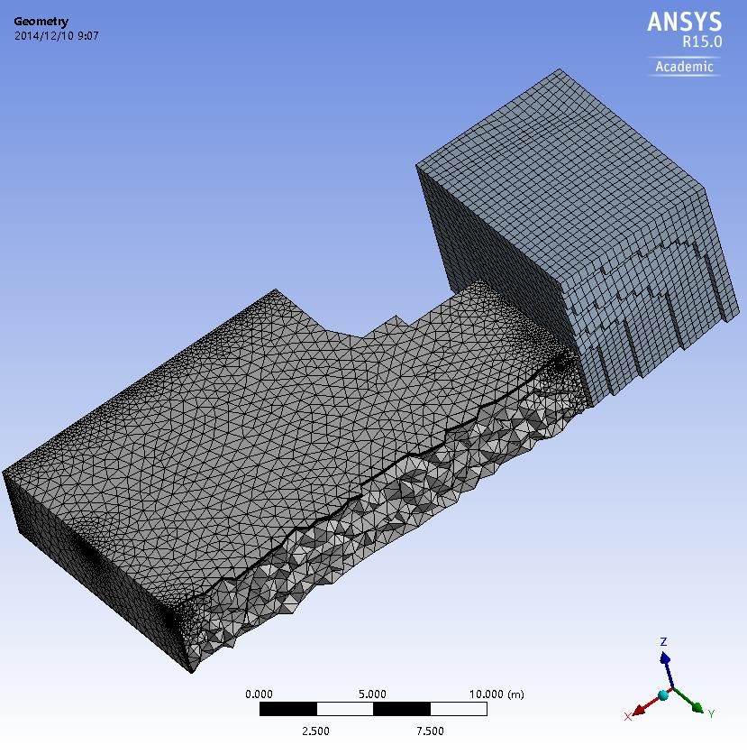
Master of Science Thesis EGI 2015: 017MSC

                                            Comparison between three different CFD
                                            software and numerical simulation of an
                                                        ambulance hall

                                                                     Ning Li
Approved                      Examiner                                  Supervisor

2015-03-05                    Joachim Claesson                          Joachim Claesson
                              Commissioner                              Contact person

                              SWECO Systems AB                          David Burman
                                                                        Liu Ting

Abstract
Ambulance hall is a significant station during emergency treatment. Patients need to be transferred from
ambulance cars to the hospital’s building in the hall. Eligible performance of ventilation system to supply
satisfied thermal comfort and healthy indoor air quality is very important. Computational fluid dynamic
(CFD) simulation as a broadly applied technology for predicting fluid flow distribution has been
implemented in this project.
There has two objectives for the project. The first objective is to make comparison between the three
CFD software which consists of ANSYS Fluent, Star-CCM+ and IESVE Mcroflo according to CFD
modeling of the baseline model. And the second objective is to build CFD modeling for cases with
difference boundary conditions to verify the designed ventilation system performance of the ambulance
hall.
In terms of simulation results from the three baseline models, ANSYS Fluent is conclusively
recommended for CFD modeling of complicated indoor fluid environment compared with Star-CCM+
and IESVE Microflo. Regarding to the second objective, simulation results of case 2 and case 3 have
shown the designed ventilation system for the ambulance hall satisfied thermal comfort level which
regulated by ASHRAE standard with closed gates. Nevertheless, threshold limit value of the contaminants
concentration which regulated by ASHRAE IAQ Standard cannot be achieved. From simulation results of
case 4.1 to 4.3 shown that the designed ventilation system cannot satisfy indoor thermal comfort level
when the gates of the ambulance hall opened in winter. In conclusion, measures for decreasing
contaminants concentration and increasing indoor air temperature demanded to be considered in further
design.

                                                   -II-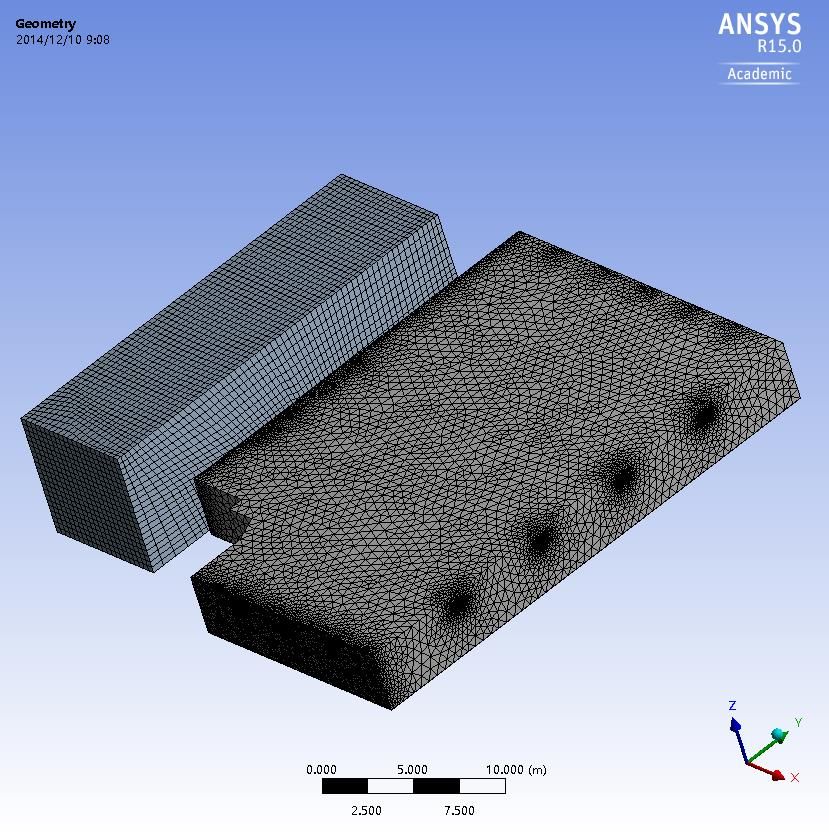
Table of Contents
Abstract ..........................................................................................................................................................................II
Acknowledgements ...................................................................................................................................................... V
List of Figures ............................................................................................................................................................. VI
List of Tables............................................................................................................................................................ VIII
Nomenclature.............................................................................................................................................................. IX
1       Introduction .......................................................................................................................................................... 1
    1.1          Background .................................................................................................................................................. 1
    1.2          Objectives ..................................................................................................................................................... 2
    1.3          Method.......................................................................................................................................................... 3
2       Numerical principle of simulation ..................................................................................................................... 4
    2.1          Governing Equations ................................................................................................................................. 4
        2.1.1             Conservation laws of fluid flow. ...................................................................................................... 4
        2.1.2             Thermal equations of wall boundary condition. ........................................................................... 4
    2.2          Turbulence modeling.................................................................................................................................. 5
        2.2.1             Different choice of k-ε Model ......................................................................................................... 5
        2.2.2             Near – Wall functions ....................................................................................................................... 7
    2.3          Meshing ........................................................................................................................................................ 8
        2.3.1             Shapes of Cell ..................................................................................................................................... 8
        2.3.2             Classification of Grids ....................................................................................................................... 8
        2.3.3             Mesh Quality....................................................................................................................................... 9
    2.4          Solver...........................................................................................................................................................10
        2.4.1             Finite Volume Method ....................................................................................................................10
        2.4.2             Upwind scheme ................................................................................................................................11
        2.4.3             SIMPLE Scheme ..............................................................................................................................11
3       Baseline model and Comparison between Software ....................................................................................13
    3.1          Data of ventilation system for baseline model. ....................................................................................13
        3.1.1             Design Concept ................................................................................................................................13
        3.1.2             Parameter of supply air diffuser ....................................................................................................13
        3.1.3             Parameter of Exhaust Grilles .........................................................................................................13
    3.2          Geometry....................................................................................................................................................14
    3.3          Meshing ......................................................................................................................................................15
        3.3.1             Meshing Independency ...................................................................................................................15
        3.3.2             Meshing Method ..............................................................................................................................17
    3.4          Numerical Setup ........................................................................................................................................19
        3.4.1             Selection of simulation models ......................................................................................................19
        3.4.2             Boundary conditions .......................................................................................................................19

                                                                                      -III-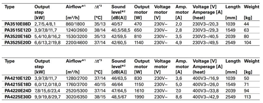
3.4.3            Solution Control...............................................................................................................................21
    3.5        Simulation results ......................................................................................................................................23
       3.5.1            Assessment of thermal comfort in an arbitrary point. ...............................................................23
       3.5.2            Velocity Distribution .......................................................................................................................24
       3.5.3            Temperature Distribution...............................................................................................................28
4      Ventilation Performance in Different Situations ..........................................................................................33
    4.1        Geometry....................................................................................................................................................33
       4.1.1            Case 2: Improved ventilation system. ...........................................................................................33
       4.1.2            Case 3: Polluted emission from tailpipes of the ambulance cars. ............................................34
       4.1.3            Case 4.1-4.3: With opened gates and installed air curtains. .......................................................34
    4.2        Meshing ......................................................................................................................................................36
    4.3        Boundary Conditions Setup ....................................................................................................................36
       4.3.1            Case 2: Improved ventilation system. ...........................................................................................36
       4.3.2            Case 3: Polluted emission from tailpipes of the ambulance cars. ............................................36
       4.3.3            Case 4.1-4.3: With opened gates and installed air curtains. .......................................................37
    4.4        Simulation Results and Analysis. ............................................................................................................38
       4.4.1            Case 2: Improved ventilation system. ...........................................................................................38
       4.4.2            Case 3: Polluted emission from tailpipes of the ambulance cars. ............................................40
       4.4.3            Case 4.1-4.3: With opened gates and installed air curtains. .......................................................43
    4.5        Optimized approaches for improving thermal comfort. ....................................................................48
       4.5.1            One more supply air diffuser on the specified wall. ...................................................................48
       4.5.2            Exhaust extraction system. .............................................................................................................49
       4.5.3            Supplement of heat in winter. ........................................................................................................49
5      Conclusion and future improvement ..............................................................................................................51
6      Bibliography ........................................................................................................................................................52
Appendix A: Data sheet/Dimension of Jet Nozzle Diffuser ..............................................................................54
Appendix B: Data and Dimension of Exhaust Grilles ..........................................................................................55
Appendix C: Data and Type of Air curtain. ............................................................................................................56
Appendix D: CO Level vs. Condition&Health Effects. .......................................................................................57

                                                                                  -IV-
Acknowledgements
Foremost I would like to express my fully gratitude to Will Sibia from SWECO systems AB, Stockholm
Sweden for giving me the opportunity to do my master thesis within such interesting and cutting edge
field by a practical project.
Specially, I would like to extend my deepest thanks to Liu Ting, who is my thesis supervisor from
SWECO in the field of CFD simulation. Encouragements, professional and theoretical supports from her
were very beneficial and helpful for me to complete the project.
Sincerely, I would also very thankful to David Berman, who is my thesis supervisor from SWECO in the
field of energy technology and ventilation systems design. Professional advices and positive feedbacks
from him supervised me done the project in the right way.
Moreover, I would like to express my grate gratitude to my supervisor, Associate Professor Joachim
Claesson, at the Royal Institute of Technology (KTH) for your fully helpful supports, responsible
feedback and all the fantastic knowledge were taught from you during the graduate study.
Finally, I am deep appreciate to my parents, my friends for their love and supports.

                                                    -V-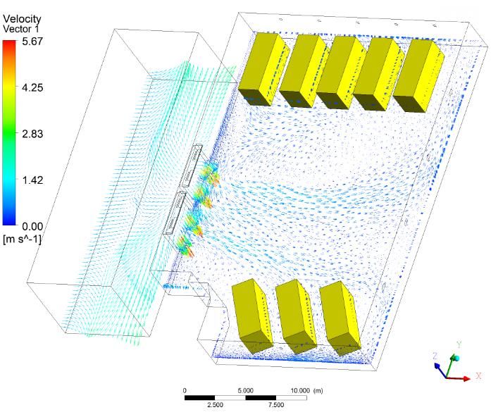
List of Figures
Figure 1, 3D layout of SÖS ambulance hall. ..................................................................................................................... 1
Figure 2, Project Outline .................................................................................................................................................... 2
Figure 3, Velocity distribution near a wall (Versteeg & Malalasekera, 2007) ............................................................... 7
Figure 4, Typical 2D control volume (Versteeg & Malalasekera, 2007). ....................................................................... 8
Figure 5, Block-structured mesh (left) and Unstructured mesh (right) of aerofoil (Versteeg & Malalasekera, 2007) ........ 8
Figure 6, Comparison between coarse, medium and fine hybrid grid. .................................................................................... 9
Figure 7, Misalignment of midpoints for skewed grid. ......................................................................................................... 9
Figure 8, Conservation of general flow variable within finite volume method (Versteeg & Malalasekera, 2007).............10
Figure 9, Evaluation of face value according to Upwind Scheme (Cho, et al., 2010). ......................................................11
Figure 10, Calculation process of SIMPLE Scheme (Versteeg & Malalasekera, 2007)...............................................12
Figure 11, Air motion of Group A outlets (ASHRAE, 1997).......................................................................................13
Figure 12, Geometry of the ambulance hall .......................................................................................................................14
Figure 13, Face sizing for air inlet (Left: Element size is 0.05m; Right: Element size is 0.03m) ..................................15
Figure 14, Face sizing for air outlet (Left: Element size is 0.1m; Right: Element size is 0.05m) ......................................16
Figure 15, Velocity distribution for the two different meshing cases. ...................................................................................16
Figure 16, Generated mesh of the ambulance hall in IESVE Microflo. ...........................................................................17
Figure 17, Generated mesh of the ambulance hall in ANSYS mesh. ................................................................................17
Figure 18, Section plane of (a) Air Inlet; (b) Air Outlet; (c) Exterior Wall; (d) Internal space ........................................18
Figure 19, Mesh metrics control of ANSYS mesh (Left: Skewness; Right: Aspect Ratio) ................................................18
Figure 20, Cell Monitor of point in Case 1.3. ..................................................................................................................23
Figure 21, PPD as a function of PMV (ISO, 1994). ....................................................................................................23
Figure 22, Thermal comfort zone display in Psychronmetric chart. ....................................................................................24
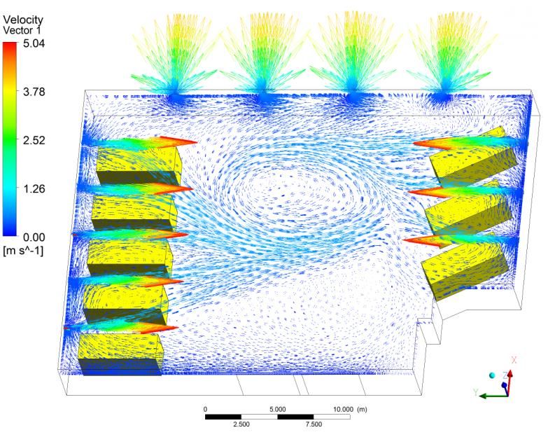
Figure 23, Vector of velocity distribution (h=3m) of case 1.1. ..........................................................................................25
Figure 24, Velocity Magnitude (h=3m) of case 1.1. (Left: 0 to 5.02m/s, Right: 0 to 1 m/s)..........................................25
Figure 25, Vector of Velocity distribution (h=1m) of case 1.1. ........................................................................................25
Figure 26, Zoomed-in views of velocity distribution at plant (h=1m).s ..............................................................................26
Figure 27, Vector of velocity distribution (h=3m) of case 1.2. ..........................................................................................26
Figure 28, Vector of velocity distribution (h=1m) of case 1.2. ..........................................................................................27
Figure 29, Vector and contour of velocity distribution (h=3m and h=1m) of case 1.3.......................................................27
Figure 30, Local mean age of air (h=1m) of case 1.3. ......................................................................................................28
Figure 31, Temperature distribution (h=1m, local temperature)........................................................................................29
Figure 32, Temperature distribution (h=1m, specified temperature). .................................................................................29
Figure 33, Temperature distribution (h=1m, global temperature) with isosurface...............................................................30
Figure 34, Temperature distribution (Left: x=3.6m, 11m and 18.3m; Right: y=10.3m, 15.5m and 21m). ...................30
Figure 35, Temperature distribution on envelop of ambulance hall.....................................................................................30
Figure 36, Temperature distribution of case 1.2. ...............................................................................................................31
Figure 37, Temperature distribution of case 1.3. ...............................................................................................................32
Figure 38, Geometry of case 2 with 4 exhaust grilles. .......................................................................................................33
Figure 39, Geometry of case 3 with tailpipe emission (Left: whole room; Right: zoomed-in to the tailpipe) .........................34
Figure 40, Configuration of air curtain which installed in case 4.1-4.3. ............................................................................34
Figure 41, Geometry of case 4.1 - 4.3. .............................................................................................................................35
Figure 42, Zoomed-in views of geometry for case 4.1-4.3. ..................................................................................................35
Figure 43, Meshing of case 4.1-4.3 (Left: Global: Right: Section cut view). ......................................................................36
Figure 44, Velocity distribution at h=3m over the ground (Local Velocity). .....................................................................38
Figure 45, Velocity distribution at h=1m (Local Velocity). .............................................................................................38
Figure 46, Zoomed-in views to figure 45. ..........................................................................................................................39
Figure 47, Temperature distribution of case 2 at h=1m (Left: local temperature, Right: Specified temperature). ................39
Figure 48, Temperature distribution of case 2 (Left: h=0.1m, isosurface=18C; Right: Room Envelope). .........................40
Figure 49, Velocity distribution of case 3 (Left: h=3m; Right: h=0.4m) .........................................................................40
-VI-
Figure 50, Velocity distribution of case 3 (h=1m). ...........................................................................................................41
Figure 51, Temperature distribution of case 3 h=0.4m (Left: Local temperature; Right: specified temperature) .................41
Figure 52, Temperature distribution of case 3 at h=1m (Specified Temperature). ..............................................................42
Figure 53, CO concentration distribution of case 3 (h=1.5m)...........................................................................................42
Figure 54, CO2 concentration distribution of case 3 (h=1.5m). .......................................................................................43
Figure 55, Velocity distribution of case 4.1 (h=1m).........................................................................................................44
Figure 56, Specified velocity of case 4.1 at h=1m (Left: Velocity 0m/s - 0.2m/s; Right: Velocity 0m/s - 1m/s). ...........44
Figure 57, Velocity distribution of case 4.1 around the opened gates. ................................................................................45
Figure 58, Temperature distribution of case 4.1 (Left=3m; Right=1m). ..........................................................................45
Figure 59, Temperature distribution of case 4.1 (Transection view at gate). .......................................................................46
Figure 60, Pressure distribution at h=1m of case 4.2(Left) and case 4.3 (Right). .............................................................46
Figure 61, Pressure change along the line of case 4.2(red line) and case 4.3 (blue line). ......................................................46
Figure 62, Velocity distribution at h=1m of case 4.2(Left) and case 4.3 (Right). .............................................................47
Figure 63,Zoomed-in Velocity distribution at h=1m of case 4.2(Left) and case 4.3 (Right). .........................................47
Figure 64, Temperature distribution at h=1m of case 4.2(Left) and case 4.3 (Right). ......................................................48
Figure 65, Install position of the additional supply air diffuser. .........................................................................................48
Figure 66, Conventional exhaust extraction system (Left) and "in ground" exhaust extraction system (Right)...................49
Figure 67, Working principle of "in ground" exhaust extraction system (Nenerman, 2014). .........................................49

                                                                            -VII-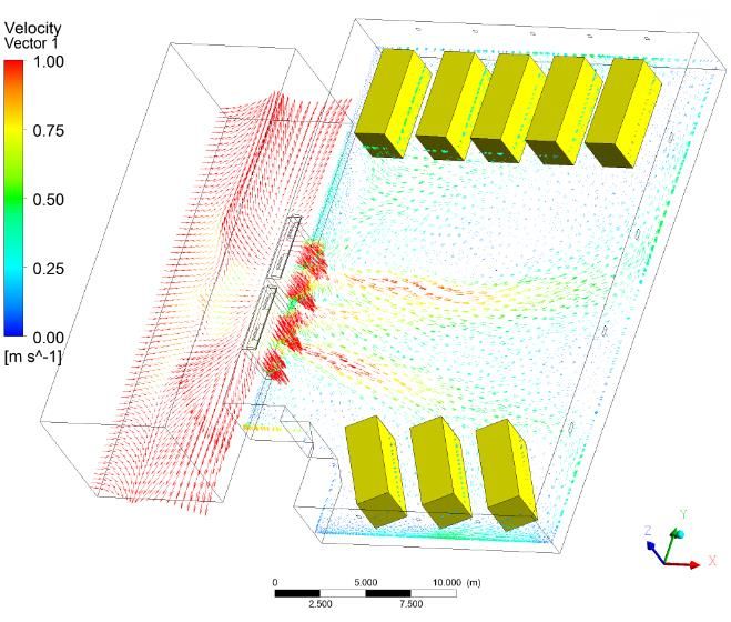
List of Tables
Table 1, Cade name of different cases.................................................................................................................................. 2
Table 2, Skewness range and cell quality (Fluent, 2006). ...............................................................................................10
Table 3, Input dimensions of geometry of the ambulance hall. ............................................................................................14
Table 4, Performance of 3D modeling for different tools. ...................................................................................................15
Table 5, Comparison of Mass flow rate and Total heat transfer rate between the two meshing cases .........16
Table 6, Statistics of mesh which generated from ANSYS mesh and IES VE – CFD Grid. .........................................18
Table 7, Performance of meshing for the three software. .....................................................................................................18
Table 8, Boundary Conditions set up in ANSYS Fluent and Star - CCM+. .................................................................20
Table 9, Solution control for the three software. .................................................................................................................22
Table 10, Performance of numerical setup for the three software. ........................................................................................22
Table 11, Thermal sensation scale for PMV Method. ......................................................................................................23
Table 12, Simulation results of the three software. ............................................................................................................32
Table 13, Different between the two types of exhaust grilles in two cases. ...........................................................................33
Table 14, Additional parameters of geometry for case 4.1 to 4.3. ......................................................................................34
Table 15, Input parameters for boundary conditions of tailpipes. .......................................................................................37
Table 16, Air curtain boundary conditions of case 4.1-4.3. ..............................................................................................37

                                                                               -VIII-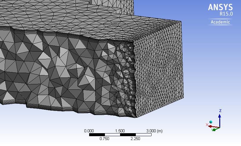
Nomenclature
Symbols
A area
Cp specific heat
Ci contaminant concentration
Cu k-epsilon model constant
g gravitational constant
hext external heat transfer coefficient
hf heat transfer coefficient of the fluid side
I tensor of unit
k thermal conductivity
P pressure
Q heat transfer rate
Sm source of mass
T Temperature
t time
u velocity
V volumetric flow rate
y+ dimensionless wall distance
dissipation rate of k
ext emissivity
k turbulence kinetic energy
Stefan-Boltzmann constant
T ,l laminar Prandtl number
T ,t turbulent Prandtl number
Φ flow variable
under-relaxation factor
near-wall temperature equation constant
ρ density
Ωij rate-of-rotation tensor
i local mean age of air
stress tensor
viscosity of molecular
Abbreviations
CFD Computational Fluid Dynamic
FVM Finite Volume Method
LMA Local Mean Age
PMV Predicted Mean Vote
PPD Percentage of Dissatisfied
RNG Re-Normalization Group
SIMPLE Semi-Implicit Method for Pressure-Linked Equations
-IX-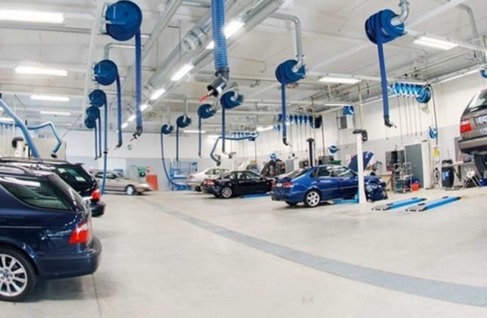
1 Introduction
1.1 Background
Numerical visualization is a platform provides a simpler way to analysis of large, complex and muti-
dimensional information. Computational fluid dynamic, also called CFD, has combined fluid mechanic
with this platform to simulate both compressible and incompressible fluid flow behavior. Distribution of
temperature, velocity, pressure, contaminant concentration and other fluid properties can be calculated
and displayed from results of CFD simulation (Stamou, et al., 2007). Output results help engineers to
improve and consummate their design quickly and effectively.
In this project, three different CFD commercial software have been employed by the author to evaluate
indoor thermal comfort of an ambulance hall which is belong to SÖS hospital renovation project from
SWECO, in Stockholm, Sweden. As defined by international standard ISO 7730, thermal comfort as
“condition of mind which expresses satisfaction of thermal environment” has explained that comfort level
need to be determined by subject method (ISO, 1994). According to the criteria ISO 7730, metabolic rate
(MET) and thermal insulation of clothing index (CLO) will be introduced for obtain thermal comfort
indexes which are predicted mean vote (PMV) and predicted percentage of dissatisfied (PPD) (ISO, 1994).
The three different CFD commercial software consist of ANSYS - Fluent, IES VE – Microflo and Star –
CCM+. Internal analyses of the ambulance hall were established by the three tools for baseline case.
Thereafter, three additional modeling cases which include improvement of ventilation system, hall with
tailpipe emissions and opened gates with natural ventilation were implemented by ANSYS – Fluent
independently.

                                Figure 1, 3D layout of SÖS ambulance hall.

Ambulance hall is a significant station during emergency treatment. Patients need to be transferred from
ambulance cars to the hospital’s building in the hall. High performance of ventilation system which supply
fresh and comfortable indoor environment is required to achieve.
As shown in Figure 1, during peak operation condition there has 8 ambulance cars parking in the hall.
Consider walls of the ambulance hall, 2 exterior wall are exposed directly to ambient environment and 2
interior walls are connected to internal corridors. For sake of simplifying the model and emphasize
performance of fluid flow within the main hall, interior rooms and internal corridors will be removed in
further 3D modeling.

                                                    1
1.2 Objectives
Two main objectives of the project had been set up.
The first objective is to build CFD modeling in three different numerical simulation software which have
been specified as ANSYS-Fluent, IES VE - Microflo and Star-CCM+. Thereafter, made comparison of
performance among these three software.
The second objective is to optimize ventilation system according to output results from baseline model,
simulate the optimized model while involving exhaust emission from the ambulance cars or natural
ventilation with opening gates.
The outline of the project is illustrated in Figure 2, the two objectives are highlighted as orange at the bottom
of the chart.
Figure 2, Project Outline
For simplify the names of each scenarios in further discussion, code name of each scenario list as in Table 1.
Table 1, Cade name of different cases.
Code Name Circumstance Description Operation Software
Case 1.1 2 exhaust grilles, without tailpipe emission, without opened gates ANSYS Fluent
Case 1.2 2 exhaust grilles, without tailpipe emission, without opened gates Star – CCM+
Case 1.3 2 exhaust grilles, without tailpipe emission, without opened gates IES VE - Microflo
Case 2 4 exhaust grilles, without tailpipe emission, without opened gates ANSYS Fluent
Case 3 4 exhaust grilles, with tailpipe emission, without opened gates ANSYS Fluent
Case 4.1 4 exhaust grilles, without tailpipe emission, with opened gates, ANSYS Fluent
Outside wind blow perpendicular into the gates with 1m/s
Case 4.2 4 exhaust grilles, without tailpipe emission, with opened gates, ANSYS Fluent
Outside wind produce negative pressure (-0.3Pa)
Case 4.3 4 exhaust grilles, without tailpipe emission, with opened gates, ANSYS Fluent
Outside wind produce negative pressure (-1Pa)
-2-1.3 Method
Numerical simulation based on computational fluid dynamic (CFD) has become broadly used for
predicting fluid behavior within the objective domain. With foreseeable fluid distribution, undesirable
fluids have the possibility to be decreased or avoided through improvement of the design.
All the simulated cases implemented in this project were built in terms of computational fluid dynamic.
However, turbulence model, boundary conditions, mesh method, simulation scheme and etc. regarding to
modelling setup have to be decided for each case.
In order to decide adaptable modeling schemes implemented during the setup, literature review from
relative scientific papers and corresponding international standards was applied in Chapter 2 and setup of
boundary conditions in Chapter 3 and 4. For comparison among the cases in different circumstances, case
studies with different boundary conditions will be analyzed and disused in Chapter 3 and Chapter 4.
Finally, improved approaches for optimizing the design of the cases will be analyzed briefly.
-3-2 Numerical principle of simulation
Numerical method for calculating air flow behavior and heat transfer performance is a more beneficial
approach compared with corresponding experiments. Both spending of time and cost can be saved
significantly. Among with multi-fields application, numerical simulation of internal air pattern of building
is developed rapidly during recent years. Detailed information of air temperature, velocity components,
and pressure drop and turbulence intensity within the modeling domain can be generated simultaneously
by CFD software.
2.1 Governing Equations
2.1.1 Conservation laws of fluid flow.
The conservation laws of fluid flow defined by Versteeg and Malalasekera (Versteeg & Malalasekera, 2007)
applies on three fundamental variable quantities which are momentum, energy and mass of fluid particle.
On the base of Newton’s second law, the sum of the forces on a fluid particle is equaled to the rate of
change of momentum. According to first law of thermodynamics, energy changing rate on a fluid particle
is equal to the work done by the particle plus the rate of heat added to it. Meanwhile, mass of fluid is
conserved. Conservation equations which required for simulation are list as followed:
For conservation of mass (Eleni, et al., 2012):
( u ) Sm (1)
t
Where Sm is the source from dispersed second phase and to be added to the continuous phase.
For conservation of momentum (Fluent, 2006):
( v) ( vv) P ( ) g F (2)
t
Where is stress tensor and expressed as below (Fluent, 2006):
v v
T
23 vI (3)
In equation (3), is the viscosity of molecular, I is the tensor of unity.
For energy equation in three dimension, four terms are associated with energy changed in the fluid particle
(Versteeg & Malalasekera, 2007):
u xx u xy u zx v xy v yy
DE x y z x y
div pu div kgradT S E (4)
Dt
v zy
w xz
w yz
w zz
z x y z
2.1.2 Thermal equations of wall boundary condition.
Five types of thermal condition which includes fixed heat flux, fixed temperature, convection, radiation
and mixed for wall boundary layer are provided by ANSYS Fluent. Considering to predict fluid flow
within the ambulance hall be more accurate, heat transfer through wall (and near wall) boundary by
conduction, convection and radiation are overall calculated.
-4-Heat transfer rate through boundary of wall by conduction:
dT
Qcond kA (5)
ds
Where k is the average thermal conductivity of material of wall.
For walls which with external radiation boundary condition, heat transfer rate expresses as:
Qrad h f Tw T f qrad ext T4 Tw4 (6)
Where both ext (emissivity of external wall) and T (temperature of external domain) are required to be
defined manually in ANSYS FLUENT and Star-CCM+.
For walls which with boundary condition of combined external convection and radiation, equation of heat
transfer rate shows as:
Qmixed h f Tw T f qrad hext Text Tw ext T4 Tw4 (7)
Where hext is the external heat transfer coefficient that to be defined according to dry-bulb temperature of
outside environment.
For equation 6 and 7, Tw is the surface temperature of the wall, h f is the heat transfer coefficient of the
fluid side, is Stefan-Boltzmann constant.
2.2 Turbulence modeling
The Navier – Stokes equations which arise from Newton’s second law is to describe viscous flow in
multiply application. A suitable model for viscous stresses component ij and pressure term are introduced
to the conservation equations. As formed by Versteeg and Malalasekera (Versteeg & Malalasekera, 2007),
the Navier – Stokes equations can be written for finite volume method (which will be discussed in section
2.5) in the most useful form as:
Du p
div gradu S Mx (8)
Dt x
For three dimensional fluid flow, the equation 8 also identically applies on y and z direction with velocity
vectors v and w .
2.2.1 Different choice of k-ε Model
Supplemented with turbulence model based on Navier – Stokes equations which implemented in practical
CFD applications, the most appropriate viscous model for numerical simulation of high Reynold number
is k-epsilon (2eqn) viscous model (Calautit, et al., 2012). In ANSYS Fluent there has three transport
equations related to k-epsilon model, the standard k-epsilon model, RNG k model and the Realizable
k Model. As demonstrated by Tsan-Hsing and et al. (Shih, et al., 1994), realizable k Model
performs the best of all versions of k Model from several validations of flows with complex
secondary features and separated flows. In Star-CCM+, there has eight different transformation equations
for choice of k turbulence model. However, only standard k turbulence model provided by IES
VE Microflo. Therefore, both standard and realizable k model have been implemented during
numerical modeling in this project.
For standard k model, the turbulence kinetic energy k and its dissipation rate , can be calculated
from equations below (Fluent, 2006):
-5- t k
k kui Gk Gb YM Sk (9)
t xi x j k x j
And
t 2
kui C1 Gk G3 Gb C2 S (10)
t xi x j x j k k
The term Gk as shown in above equations is the production of turbulence energy due to mean velocity
gradients which defined as:
u j
Gk ui'u 'j (11)
xi
The term Gb as shown represents production of turbulence energy due to buoyancy effect which defined
as:
t T
Gb gi (12)
Prt xi
The viscosity of turbulence flow, t is calculated by combination of k and as follow:
k2
t C (13)
And for constants in the equations 9 and 10 are listing as (Markatos , 2004):
C1 = 1.44, C2 =1.92, C =0.09, k =1.0 and =1.3
For realizable k model, the turbulence kinetic energy k and its dissipation rate , can be calculated
from equations below (Shih, et al., 1994):
t k
k ku j Gk Gb YM Sk (14)
t x j x j k x j
And
t 2
u j C S C C1 C3 Gb S (15)
t x j x j x j
1 2
k v k
Where,
k
C1 max 0.43, , S , S 2 Sij Sij (16)
5
Differ from standard k model, C is not constant any more, it need to be computed from:
1
C
kU * (17)
A0 AS
Where,
U * Sij Sij ij ij (18)
And
ij ij 2 ijkk ; ij ij ijk k ; A0 =4.04, AS 6 cos
Where,
-6-1 u j ui
1 Sij S jk S kt
cos 1 6W , W , S Sij Sij , Sij (19)
3 S
3
2 xi x j
And for constants in the equations 14 and 15 are listing as (Fluent, 2006):
C1 = 1.44, C2 =1.9, k =1.0 and =1.2
The generation of the turbulence kinetic energy is calculated in the same way for both standard and
realizable k model except for value of constants, with the same Gk and Gb representation which
shows in equation 11 and 12.
2.2.2 Near – Wall functions
Gradient of velocity changed in near-wall region is usually strong for no-slip walls. As shown in Figure 3,
according to mathematical and experiments analysis, near-wall region can be separated into two layers
which are laminar flow (linear sublayer) and turbulence flow (Versteeg & Malalasekera, 2007). Regions are
subdivided by point P shown in Figure 3.
Figure 3, Velocity distribution near a wall (Versteeg & Malalasekera, 2007)
When value of y is larger than 11.63 (above point P), mean velocity of turbulence flow is considered to
be in log-law region and can be yielded as:
ln Ey
1
U (20)
Where y+ shows as equation below:
yu *
y (21)
v
And temperature distribution for turbulence flow in near wall region is computed as (Launder & Spalding,
1973):
T T ,t u P T ,l (22)
T , t
Where in equation 20 and 21, is 0.4187, E is constant shear stress 9.793 for smooth walls, T ,l and
T ,t are laminar and turbulent Prandtl number.
In order to obtain the most accurate velocity profile in near-wall region, not only computational equations
but also intensive mesh with high equality are required to be applied during the simulation. Therefore,
inflation layers which can help to improve mesh quality will be discussed later in following chapters.
-7-2.3 Meshing
2.3.1 Shapes of Cell
Mesh quality during pre-processing is very significant for CFD simulation results. Grid of simulation
object is generated upon the completed geometry. Both polygonal and polyhedral mesh is practicably
applied. As some simple examples list by (Versteeg & Malalasekera, 2007) and shown in Figure 4, different
shapes of control volumes are used for surface meshing (2D). And in volume meshing (3D), triangular or
quadrilateral surface elements helps to bind the 3D control volume.
Figure 4, Typical 2D control volume (Versteeg & Malalasekera, 2007).
2.3.2 Classification of Grids
Different types of grids implement on different shapes of geometry. There are three main classifications
of grid commonly used for meshing the object. Block-structured grid, unstructured grid and hybrid grid.
For block-structured grid, which have the most space efficient, the equations are simpler to be discretized
and it is very recommendable for solving complex geometries. As explained by Versteeg and Malalasekera
(Versteeg & Malalasekera, 2007), unstructured grid is being advantage that no implicit structure of co-
ordinate lines is created by the grid and this type of mesh is also simple to concentrated wherever
necessary. Therefore, time spent for mesh generation and mapping is much shorter through unstructured
grid. Appearances of block-structured and unstructured grid are shown in Figure 5.
Figure 5, Block-structured mesh (left) and Unstructured mesh (right) of aerofoil (Versteeg & Malalasekera,
2007)
-8-A mixture of structured gird and unstructured grid can be classified as hybrid grid. In 2D, the mixture
contains of triangular and quadrilateral elements and in 3D the mixture combined tetrahedral and
hexahedral elements for calculation of fluid flow (Crippa, 2011). In Figure 6, comparison between coarse,
medium and fine hybrid grid of aerofile is shown from left to right.
Figure 6, Comparison between coarse, medium and fine hybrid grid.
Observed from figure above, region near the boundary layer have been generated to a high mesh quality
by creating structured grids. Within near wall regions the velocity changed very fast, for capture right
gradient of the change, inflation layers is required to be added near the boundary layers.
In this project, for achieving an accurate and time efficient meshing model, hybrid grids which combined
both advantages of structured and unstructured grids was selected to be implemented during pro-
processing.
2.3.3 Mesh Quality
As defined by user guide of ANSYS Fluent (Fluent, 2006), skewness is the different between shape of cell
and shape of an equilateral cell of equivalent volume. For instance, as illustrated by Versteeg and
Malalasekera (Versteeg & Malalasekera, 2007) shown in Figure 7, when the line PA and ab is not intersect at
the midpoint m of ab and the grid is non-orthogonal, lower accuracy of the simulation will be obtained
due to the increased skewness. Therefore, in order to get a more precise results, control of skewness
during meshing is very important.
Figure 7, Misalignment of midpoints for skewed grid.
Different cell quality can be indexed by different range of skewness value. According to reference given by
ANSYS, ranks of cell quality from degenerate to equilateral with corresponding range of skewness lists in
Table 2:
-9-Table 2, Skewness range and cell quality (Fluent, 2006).
Skewness Cell Quality
1 degenerate
0.9 – <1 Bad(sliver)
0.75 – 0.9 poor
0.5 – 0.75 fair
0.25 – 0.5 good
>0 – 0.25 excellent
0 equilateral
The other control index of mesh quality is ASPECT RATIO. Which is the ratio between the length of
longest edge and the length of the shortest edge. This control method of mesh quality is the only supplied
selection for IES VE - Microflo.
2.4 Solver
2.4.1 Finite Volume Method
Distinguish with finite element and finite difference method, Finite Volume Method (FVM) which is the
most widely applied for final solution method of computational fluid dynamic today. As described by
Charles (Hirsch, 2007) finite volume method is given to technique which is directly discretize integral
formulation of the conservation laws in physics space. Once the geometry was meshed and divided into
small cells which is also called control volume, the integrated governing equations of fluid flow within
computational domain are satisfied with conservation of each relevant properties for the control volume.
Distinct connections between the underlying physical conservation principle forms and the numerical
algorithm makes finite volume method be simpler than other methods (Versteeg & Malalasekera, 2007).
The conservation of a general flow variable Φ within finite volume method can be expresses in words and
shows in equation in Figure 8 (Versteeg & Malalasekera, 2007).
Figure 8, Conservation of general flow variable within finite volume method (Versteeg & Malalasekera, 2007).
As shown in Figure 8, the total net change of the flow variable due to convection, diffusion and inside source
term is contained by change in the control volume with respect to time. In reality simulation, the involved
physical phenomena are usually non-linear and diverse, iterative solution approach is demanded (Cehlin,
2006).
Concerning the three CFD codes which are employed in this work, the Finite Volume Method (FVM) is
the common solver that applies for all three participated software.
-10-2.4.2 Upwind scheme
Differ from central differencing scheme, the upwind differencing scheme has the capability to identify the
flow direction. As shown in figure below, the convective quantities are defined as ( ) f . The direction of
the fluid is flow from cell i to cell j (Cho, et al., 2010).
Figure 9, Evaluation of face value according to Upwind Scheme (Cho, et al., 2010).
For the first order upwind differencing scheme, value of convective qualities are equal to the value at the
previous node as shown in follow:
i if f 0
( ) f (23)
j if f 0
For the second order upwind differencing scheme, assumption of value for convection qualities is
replaced by the linear distribution. Higher accuracy is consequently obtained at the cell faces by
implemented Taylor series expansion to the cell centers (Barth & Jesperson, 1989):
i i dx fi if f 0
( ) f (24)
j j dx fj if f 0
Where the factor dxf is indicating the vector is from center of the cell to the center of the face.
In this project, second upwind differencing scheme was employed for spatial discretization of momentum,
turbulent kinetic energy, and turbulent dissipation rate and energy computation.
2.4.3 SIMPLE Scheme
SIMPLE scheme was selected for pressure-velocity coupling scheme in solution methods. SIMPLE is
represented for Semi-Implicit Method for Pressure-Linked Equations. The initial value of pressure and
velocity for calculation is guessed as p* and u* to initiate the calculation process (Versteeg & Malalasekera,
2007). To obtain the correct pressure and velocity field, the correction factor of pressure p’ and u’ are
introduced:
p new p* p p ' (25)
For a two-dimensional laminar steady state flow, the correct velocity unew and vnew can be improved from
the equations:
u new u* u u ' (26)
-11-v new v* v v ' (27)
The defined as under-relaxation factor for iterated calculation. This factor which taken from 0 to 1
helps to improve the iterative process move forward while influence the stability of the fluid flow
calculation. If the under-relaxation factor equal to zero, there will be no correction applied to the
computation. If the under-relaxation factor equal to one, the guessed field of pressure and velocity is far
away from the final solution.
According to the diagram which was illustrated by Versteeg and Malalasekera (Versteeg & Malalasekera,
2007), the computed process of SIMPLE algorithm is shown as Figure 10,
Figure 10, Calculation process of SIMPLE Scheme (Versteeg & Malalasekera, 2007).
The initial guessed values were assumed and set manually during solution initialization. The more
realizable of the initial value, the faster of the convergence time cost. Each iteration takes from step 1 to
step 4, convergence absolute criteria for residual of each equations were set in monitor. When the
residuals did not achieve the criteria, value of convective qualities were replaced by the corrected value for
the next iteration until the criteria had been achieved.
-12-3 Baseline model and Comparison between Software
In this chapter, baseline model would be initially built by ANSYS Fluent. According to ventilation system
had been implemented on ambulance hall of NKS (Nya Karolinska Solna) hospital, similar design concept
would be applied on the baseline model of the SÖS (Södersjukhuset) ambulance hall. Baseline models
which set up by IES VE – Microflo and Star – CCM+ were also discussed later in this chapter.
3.1 Data of ventilation system for baseline model.
3.1.1 Design Concept
According to requirements of design which supplied by the constructor of NKS hospital, the minimum
indoor air temperature of an ambulance hall which located in Stockholm, Sweden is not allowed be lower
than 18 ℃ and the air flow level should not lower than 3 l/s-m2.
As classified by ASHRAE Handbook (ASHRAE, 1997), group A of diffuser type that is “Diffusers
mounted in or near the ceiling that discharge air horizontally” is very popular to be applied in commercial
implementations. Figure 11 gives air stream performance of group A when the air jet diffusers are installed
on the opposite walls. Diffusers in this project were also installed for providing colliding airstreams.
Figure 11, Air motion of Group A outlets (ASHRAE, 1997).
3.1.2 Parameter of supply air diffuser
The total area of the ambulance hall is 645.12 m2. Therefore, minimum total volumetric flow rate is
obtained as 1935.36 l/s. Length of the hall is around 31m, read from data sheet of jet nozzle diffuser
which obtained from supplier and listed in Appendix A, considering isothermal throw length (L0.2) of
each diffuser type, APL/N -250 with L0.2 equal to 15m was selected for air supply of ventilation system.
The volumetric flow rate of supply air from APL/N – 250 is 250 l/s as list in Appendix A. In order to
reach the minimum total volumetric flow rate of the ambulance hall, 8 units of air diffuser required to be
installed consequently.
3.1.3 Parameter of Exhaust Grilles
The baseline model is setting as no natural ventilation and tailpipe emission involved, in accordance with
mass balance equation which is input equals to output, the total volumetric flow rate of exhaust grilles is
same to the value of supply air diffuser. According to data sheet of exhaust grilles from Appendix B, two
units of AGC - 800×400 with qv equal to 1099 l/s have been chosen for installation.
-13-3.2 Geometry
With removed internal rooms and corridor, the geometry of the ambulance hall for further simulation is
drew and shows in Figure 12. There are maximum of eight ambulance cars parking in the hall which
displayed as rectangular boxes in the room. Smaller squares that locating on both north and south face of
the room envelope are the eight supply air diffusers. Two larger rectangles that locating on the east face of
the room envelope are the exhaust grilles. The two faces which showing on the west wall are the gates of
the ambulance hall.
Figure 12, Geometry of the ambulance hall
Shape of the jet nozzle diffusers is designed as circle by manufacture as shown in Appendix A, but
because of limitation of IES VE – Microflo, which cannot draw circle for representing air inlet in the
software, quadrate with same area is used for representing faces of supply air diffusers instead.
For 3D modeling of geometry of the ambulance hall, input dimensions which obtained from constructor
lists in Table 3.
Table 3, Input dimensions of geometry of the ambulance hall.
Ambulance Hall Length 31.407 m
Width 21.892 m
Height 3.8 m
Ambulance Car Length 5.477 m
Width 1.927 m
Height 2.5 m
Gate Width 4m
Heigth 3.1 m
Supply air diffuser (Air Inlet) Length 0.224 m
Width 0.224 m
Height of installed positions 3m
above the floor
Exhaust Grille (Air Outlet) Length 0.776 m
Width 0.376 m
Height of installed positions 3m
above the floor
Different geometry modelers is bound with each CFD software. For 3D modeling tools which had been
employed by author to build the same geometric model of the ambulance hall, grade level of modeling
efficiency according to the author’s using experience is shown as in Table 4:
-14-Table 4, Performance of 3D modeling for different tools.
3D Modeling
ANSYS Fluent IES VE - Microflo Star – CCM+
Tools DesigeModeller SpaceClaim ModelIT SketchUp 3D-CAD SpaceClaim
(Default) (collaborate) (Default) (Plug-In) (Default) (export .stp
file )
Manipulate 3 5 1 4 2 5
Difficulty of
Interface
Degree of 3 5 1 4 2 5
precision
Time 3 4 1 5 2 4
Spending
In Table 4, software performance is divided into 5 level. 3D modeling tool with the best efficiency and
performance gained 5 point, on the contrary, tools with less satisfaction are gained lower points. From
results of comparison, the geometry modeling tools of ANSYS has the capability to performance easier,
more intuitively and faster than the rest. Since the main functions of IES VE is to establish energy
performance for buildings, ModelIT is easier to be used for build building block without complex
geometry.
During simulation of baseline models, both ANSYS Fluent and Star – CCM+ shared same geometry file
which built by SpaceClaim, and SketchUp 2014 was employed for 3D modeling to IES VE – Microflo.
3.3 Meshing
3.3.1 Meshing Independency
Before continue with different circumstances of the ambulance hall, meshing independency study of
baseline scenario is strongly recommended to be implemented for obtain a more confident simulated
results. Therefore, two simulations of case 1.1, which is the baseline model modeled by ANSYS Fluent,
were generated as different number of cells. One with 380587 cell elements, the other one has 505743 cell
elements.
The following two groups of figures are shown face sizing for boundary face of supply air diffuser (Air
Inlet) and Exhaust Grilles (Air Outlet). In the baseline cases, four places were applied as specified face
sizing, where are air inlet faces, air outlet faces, exterior walls and the two gates. Since air temperature and
velocity are changed significantly at these locations, quality of mesh at these locations required higher than
the rest.
Figure 13, Face sizing for air inlet (Left: Element size is 0.05m; Right: Element size is 0.03m)
-15-Figure 14, Face sizing for air outlet (Left: Element size is 0.1m; Right: Element size is 0.05m)
After both simulation completed, results of mess flow rate and total heat transfer rate of each boundary
face were computed and list in Table 5.
Table 5, Comparison of Mass flow rate and Total heat transfer rate between the two meshing cases
Model with 380587 cells Model with 505743 cells
Air Inlets 2.449327 2.449327
Mass Flow Air Outlets -2.44993 -2.44925
Rate (kg/s) Net Results 1.73*10-5 7.22*10-5
Ambulance Car 0 0
Exterior wall -1961 -1957
Total Heat Gates -1001 -997
Transfer Rate Air Inlet -13285 -13285
(W) Interior wall -52 -43
Air Outlet 16258 16186
Net Results -41 -97
Percentage 0.25% 0.6%
Results of indoor air flow velocity (vector) also shown in Figure 3, for helping to verify the simulation results
are independent from current degree of mesh quality.
Figure 15, Velocity distribution for the two different meshing cases.
Both results from Table 5 and in Figure 15 have illustrated there has only extremely small differences between
the two meshing cases. The simulation results are independent from mesh quality at this degree.
-16-You can also read