Multiscale dynamic human mobility flow dataset in the U.S. during the COVID-19 epidemic - Nature
←
→
Page content transcription
If your browser does not render page correctly, please read the page content below
www.nature.com/scientificdata

               OPEN           Multiscale dynamic human mobility
Data Descriptor               flow dataset in the U.S. during the
                              COVID-19 epidemic
                                                               1✉
                              Yuhao Kang1, Song Gao                , Yunlei Liang1, Mingxiao Li      1,2,3
                                                                                                             , Jinmeng Rao1 & Jake Kruse1

                              Understanding dynamic human mobility changes and spatial interaction patterns at different
                              geographic scales is crucial for assessing the impacts of non-pharmaceutical interventions (such as
                              stay-at-home orders) during the COVID-19 pandemic. In this data descriptor, we introduce a regularly-
                              updated multiscale dynamic human mobility flow dataset across the United States, with data starting
                              from March 1st, 2020. By analysing millions of anonymous mobile phone users’ visits to various places
                              provided by SafeGraph, the daily and weekly dynamic origin-to-destination (O-D) population flows are
                              computed, aggregated, and inferred at three geographic scales: census tract, county, and state. There
                              is high correlation between our mobility flow dataset and openly available data sources, which shows
                              the reliability of the produced data. Such a high spatiotemporal resolution human mobility flow dataset
                              at different geographic scales over time may help monitor epidemic spreading dynamics, inform public
                              health policy, and deepen our understanding of human behaviour changes under the unprecedented
                              public health crisis. This up-to-date O-D flow open data can support many other social sensing and
                              transportation applications.

                              Background & Summary
                              The outbreak of the novel coronavirus disease SARS-CoV-2 (also known as COVID-19) in December 2019 has
                              become a global threat to public health and human societies. Thus far, more than 25 million people have been
                              infected by the virus with more than eight hundred thousand death cases globally1. To contain the transmission
                              of the COVID-19, social distancing has been proved as the most effective non-pharmaceutical intervention2–4,
                              and governments have applied various policies to reduce human mobility and restrict large gatherings, such as
                              regional lockdowns5, stay-at-home orders6,7, and travel restrictions8,9. Tracking dynamic human mobility changes
                              and spatial interaction patterns is therefore a prerequisite for measuring the effects of human mobility and inter-
                              ventions on predicting the virus spread10,11. Several recent works have employed human movement flow matrices
                              in understanding spatial interaction changes and social impact, and enabling network-based epidemic mod-
                              els to project the numbers of COVID-19 infected population in different countries such as China, Japan, Italy,
                              France, Chile, and UK12–22, which requires up-to-date inbound and outbound human movement flow informa-
                              tion. However, there is no such openly and timely updated human movement origin-to-destination (O-D) flow
                              matrix data at a fine spatiotemporal resolution available in many other countries where researchers can only use
                              historical O-D survey data and other proxies as a compromise23.
                                  Human mobility has been widely studied in multiple disciplines such as geography, transportation, urban
                              planning, physics, computer sciences, and public health24. It reflects patterns about how people move from
                              place to place and serves as an indicator of human behaviour and underlying socioeconomic environments.
                              With the rapid development of information and communication technologies (ICT) and GPS embedded devices,
                              large-scale mobile phone data provides an unprecedented opportunity in tracking human trajectories, which
                              benefits research about human mobility patterns. Existing studies have used such data to investigate basic laws
                              governing human movements25,26, model regional transportation connectedness and economy27,28, describe daily
                              commuting flows29, compute urban vibrancy30,31, inform public health policy4,17,32, and understand spatial inter-
                              action patterns33–35.

                              1
                               GeoDS Lab, Department of Geography, University of Wisconsin-Madison, Madison, WI, 53706, United States.
                              2
                               Institute of Geographic Sciences and Natural Resources Research, Chinese Academy of Sciences, Beijing, 100101,
                              China. 3School of Architecture and Urban Planning, Shenzhen University, Shenzhen, 518061, China. ✉e-mail: song.
                              gao@wisc.edu

  Scientific Data |   (2020) 7:390 | https://doi.org/10.1038/s41597-020-00734-5                                                                1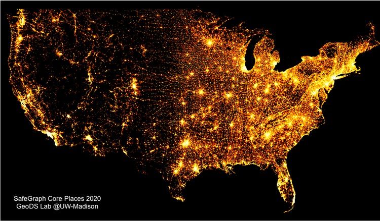
www.nature.com/scientificdata/ www.nature.com/scientificdata
a. TRACK PLACE VISITS b. COMPUTE VISITOR FLOWS
Daily CBG to CBG Visitors
Mobile Phone Data User Trajectory Place Visitors
Weekly POI to CBG Visitors
c. MULTI-SCALE AGGREGATION
d. INFER POPULATION FLOWS
Dynamic SafeGraph Census Populaon
Populaon = Visitor x
Flows Flows SafeGraph Devices
Census Tract to
County to County State to State
Census Tract
Fig. 1 The data processing framework for the mobility flow dataset production: (a) track place visits; (b)
compute visitor flows; (c) multi-scale aggregation; and (d) infer population flows.
As pointed out by several recent studies10,36–38, human mobility data plays a key role and serves as data foun-
dation in the fight against the COVID-19 pandemic. Although companies such as Descartes Labs (https://www.
descarteslabs.com/mobility/)39, Apple (https://covid19.apple.com/mobility), Google (https://www.google.com/
covid19/mobility/)40, and Facebook (https://dataforgood.fb.com/docs/covid19/)41, have released a set of near
real-time mobility-related open datasets for monitoring human mobility changes and social distancing behaviour
during the COVID-19 period, these datasets are lacking in three respects. First, human mobility flow matrices,
which describe movement patterns from origin geographic units to destination regions, are often unavailable,
even though such O-D paired flow matrices are incredibly valuable for epidemic transmission modeling and
spatial-social interaction measurements2,10,19,42,43. For instance, only aggregated mobility indices (such as median
travel distance and foot-traffic) at a specific region is provided by the Descartes Labs, Apple, and Google mobility
datasets. Second, there is a lack of fine-resolution datasets regarding the privacy-accuracy trade off. Most openly
available datasets aggregate mobility patterns to the state, county or city scale, while higher spatial resolution (e.g.,
census tract) datasets, which provide more detailed human mobility patterns, are necessary to more accurately
characterize heterogeneous human mobility changes within cities or intra-counties during the pandemic38. Third,
the mobile phone or other sensor data-driven mobility patterns often only provide a sample (e.g., 10%) of the
entire population. There is no entire-population-level estimated flow data.
To address the limitations of existing mobility databases, we introduce an openly available dataset that pro-
vides an estimation of dynamic population flows at multiple spatial scales (at the census tract, county, and state)
and temporal resolutions (daily and weekly) across the U.S. during the COVID-19 pandemic considering the
findability, accessibility, interoperability, and reusability of data44. A similar mobility dataset has been released
by researchers from Italy45, while we focus on the mobility in the U.S.. The O-D format dataset is generated
by tracking millions of anonymous mobile phone users’ trajectories collected by SafeGraph46. When produc-
ing the dataset, great efforts were taken to protect personal privacy by aggregating to various geographic scales
so that individual information cannot be traced. Other public datasets, such as the the American Community
Survey (ACS) commuting flows and the Descartes Lab COVID-19 mobility dataset are then compared to illus-
trate the reliability of the produced dataset. Such an up-to-date dataset can be a useful supplement in human
mobility observation. It can be used not only in the fight against the COVID-19 pandemic, but also to benefit
other researches and applications such as emergency response47,48, urban planning49, and population migration50.
Methods
Figure 1 illustrates detailed processing steps for how this human mobility flow dataset is generated. The dynamic
population O-D flow matrices are estimated using mobile phone location data provided by SafeGraph and demo-
graphic data retrieved from the ACS. Based on millions of anonymous mobile phone user visits to various places
tracked by SafeGraph, two types of visitor flows, namely daily census block group (CBG) to CBG visitors and
weekly CBG to point of interest (POI) visitors are computed, respectively. After spatially joining the place visitors
to the administration regions, the visitor O-D flows are computed at three different spatial scales: census tract,
county, and state, which are used to provide multi-scale views of human mobility and spatial interactions patterns
between different places. Since the number of mobile phone users detected by SafeGraph is about 10% sample of
the entire population51, we further employ the ACS population data with mobile phone data samples to infer the
population level of dynamic O-D flows.
Track place visits. The place visitor patterns are retrieved from the SafeGraph COVID-19 Data
Consortium46. Millions of anonymous GPS pings collected from numerous mobile applications are tracked and
then cleaned to remove noise. Then, users’ home places are estimated and aggregated (e.g., at the level of a CBG),
and those users’ visits from home places to POIs are tracked. POIs are the primary venue for tracking place
foot-traffic by SafeGraph, while CBG is one of the fine-resolution geographical units the United States Census
Scientific Data | (2020) 7:390 | https://doi.org/10.1038/s41597-020-00734-5 2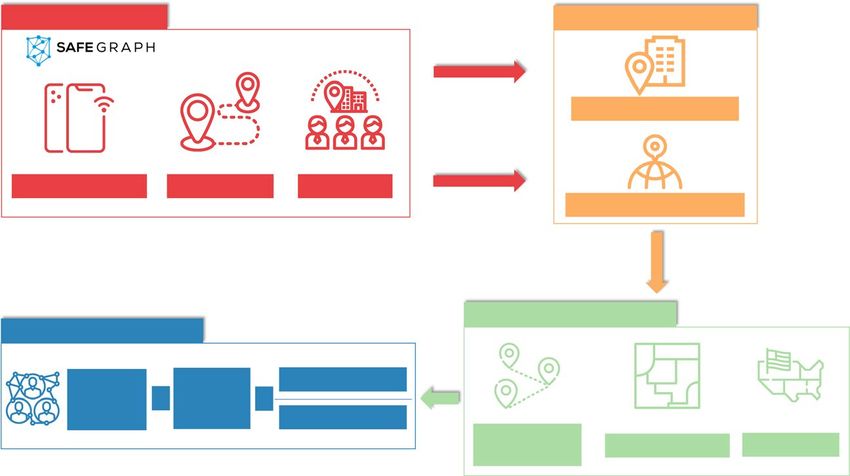
www.nature.com/scientificdata/                                                                          www.nature.com/scientificdata

                            Fig. 2 Spatial density distribution of places collected by SafeGraph across the whole United States; the
                            visualization is created using the DataShader package, Python 3.7.

                             Type                             Origin         Destination     Visitors
                             (A) daily CBG to CBG visitors    0123456789xx   0123456798xx    50
                             (B) weekly CBG to POI visitors   0123456789xx   sg:012345xx     10

                            Table 1. A sample record of: (A) daily CBG to CBG visitors; (B) weekly CBG to POI visitors.

                            Bureau used for publishing demographic and socioeconomic data. A home place of a user refers to his/her most
                            common nighttime location during the last six weeks. For each day, GPS pings of each device are clustered and
                            only those clusters during nighttime hours (6 pm - 7am local time) are kept. The CBG with the most clusters in
                            that day is recorded. Based on this, the most frequent CBG over the last six weeks that reflects the primary night-
                            time location is used as the “home location” for each user. By aggregating home places to CBGs, user privacy can
                            be protected as no individual records can be traced and accessed52.
                                Active users’ visits to POIs are produced with a similar strategy. Using several clustering methods such as
                            density-based spatial clustering for applications with noise (DBSCAN)53, GPS pings are grouped together in
                            which each cluster contains a set of potential POIs and associates with CBGs. The best place for a given cluster
                            is classified by performing machine learning methods involving several entangled features. Thereby each user’s
                            visits from home place to various POIs and CBGs are identified54.
                                In total, there are more than 5 million POIs stored in the database, as well as more than 220 thousand CBGs
                            retrieved from the ACS. The spatial density distribution of POIs across the Contiguous United States is mapped
                            in Fig. 2, which shows that places cluster in major cities and are generally located along streets. The more places,
                            the brighter the region in the map.

                            Compute visitor flows.         Two major human mobility flow metrics are employed in data production, and
                            are denoted as daily CBG to CBG visitor flows and weekly CBG to POI visitor flows. In the daily CBG to CBG
                            visitor flows metric, each row contains an origin CBG and a destination CBG, as well as the number of mobile
                            phone-based visitor flows from the origin CBG to the destination CBG. Every day, the number of unique mobile
                            phone users who live in the origin CBG and visits to the destination CBG are recorded. More specifically, GPS
                            pings of each user are clustered first. Only those clusters (i.e., not a single trajectory point) with a duration of at
                            least one minute are counted as a “visit”54. By doing so, the daily mobile phone-based visitor flows between CBG
                            and CBG are grouped and summed up. A sample record of the daily CBG to CBG visitor flows is included in
                            Table 1.
                                For the weekly CBG to POI visitor flows metric, different from the daily CBG to CBG visitor flows metric which
                            aggregates visitors between origin CBG and destination CBG directly, it provides a mapping of CBGs to POIs. In
                            other words, the number of unique visitors who live inside the origin CBG and visit the destination POI in one
                            week are counted. A sample record of the weekly CBG to POI visitor flows is also included in Table 1.

                            Multiscale aggregation. The two mobile phone-based visitor flows metrics (from CBG to CBG and from
                            CBG to POI) are both processed at the CBG scale. After obtaining these two metrics, all data are further aggre-
                            gated into three different spatial scales: census tract, county, and state. The motivations for providing data prod-
                            ucts at multiple spatial scales are discussed as follows. First, using coarser/finer analysis unit may lead to different
                            outputs, which is known as the scale effect. As an important and fundamental concept in geography, the scale
                            effect exists in almost all geographic phenomena55,56, including human mobility patterns57. Providing a multiscale
                            flow dataset allows us to have a more comprehensive view of human mobility and spatial interaction patterns.
                            Second, various research projects may acquire data at different spatial scales, depending on the usage. For exam-
                            ple, for research focusing on a macro view of spatial interactions, state or county scale data might be more suitable
                            as it reflects general regional mobility patterns, while census tract scale data can be used for describing a micro
                            view of human movement patterns such as within cities. Also, considering the data size-accuracy trade-off (i.e.,
                            the higher the spatial resolution, the higher the accuracy but the larger the data size is), providing a multiscale
                            dataset enables users to download the data that fit their own needs. Third, although the daily CBG to CBG visitor
                            flows and weekly CBG to POI visitor flows have been computed at the CBG scale, which is a finer spatial scale,
                            aggregating them to coarser-level can preserve the data privacy better. Therefore, the O-D flow dataset is gener-
                            ated at three geographical scales, respectively. To do so, we assign census tract, county, and state’s geographically

Scientific Data |   (2020) 7:390 | https://doi.org/10.1038/s41597-020-00734-5                                                                     3
www.nature.com/scientificdata/ www.nature.com/scientificdata
unique identifier to each origin CBG and destination CBG that they belong to, and group all records according to
the O-D pairs. In total, there are 74,001 census tracts, 3,219 counties, and 50 states & Washington D.C. & Puerto
Rico at each spatial scale for aggregation in the U.S. The aggregated mobile phone-based weekly CBG to POI visi-
tor flows and the daily CBG to CBG visitor flows are termed as weekly visitor flows and daily visitor flows hereafter,
respectively.
Infer dynamic population flows. The above-mentioned visitor flows at the three spatial scales are calcu-
lated based on mobile phone users detected by SafeGraph, not on the entire population. These users account for
about 10% to the entire population in the U.S., and the sampling ratio of unique mobile devices to population var-
ies across CBGs to CBGs51. Existing studies have shown that a good representative sample of the entire population
can reflect general human mobility patterns26. Also, short-term mobility and long-term migration are affected by
multiple factors such as physical travel costs (distance, time, and money), economic and health benefits, social
and political frictions34,58–62. Given that SafeGraph’ samples are highly correlated with the true Census popula-
tions regarding several socio-economic attributes51, we aim to infer the short-term population-level dynamic
mobility flows during the COVID-19 pandemic as it is important to accurately estimate meta-population infec-
tion cases and in other human mobility applications4,19,24. To do so, by utilizing the official ACS population data
with mobile phone visitor patterns, the dynamic population flows are inferred using the following equation:
pop(o)
pop _flows(o , d ) = visitor _flows(o , d ) ×
num_devices(o) (1)
where pop_flows(o , d ) is the estimated dynamic population flows from geographic unit o to geographic unit d,
visitor _flows(o , d ) is the computed mobile phone-based visitor flow from o to d, pop(o) indicates the population
at the geographic unit o extracted from the ACS, and num_devices(o) refers to the number of unique mobile
devices residing in o. In addition, we also compare the estimation results with a gravity model and a radiation
model (see more details in the “Technical Validation” section).
Data Records
We have produced two data products: weekly flow data and daily flow data, both of which are provided at the
census tract, county, and state scales, starting from March 1st, 2020. A static copy of the dataset has been uploaded
on Figshare63, while the live version of the dataset will be kept up-to-date with new data stream and can be down-
loaded from an open data repository on Github: https://github.com/GeoDS/COVID19USFlows. Data provided in
this repository are separated into two folders daily_flows and weekly_flows to store daily flow data and weekly flow
data, respectively. The two folders are organized according to the geographic scale, where ct2ct indicates flows
between census tract to census tract, county2county refers to flows between county to county, and state2state con-
tains flow data that originate from one state to others. All files are stored in a comma-separated values (CSV) for-
mat, which has been widely used for storing, transferring, and sharing data publicly. File names are formatted as
{data_type}_{spatial_scale}_{date}.csv, e.g., weekly_ct2ct_03_02.csv and daily_state2state_04_19.csv. Specifically,
for weekly flow data, the dates in file name refers to the date of the Monday in that week but summarize all mobil-
ity flows in that week from Monday to Sunday. Since the file size of flow data at the census tract scale exceeds the
GitHub disk limit, each flow data file is split into 20 subfiles (that can be merged after downloading). The daily
and weekly aggregated directional flows are coded by pairwise origin to destination units using geo-identifiers
(GEOIDs). The GEOIDs are numeric codes that uniquely identify different administrative levels (e.g., census
tract, county, and state) in the U.S. Census Bureau data portal64. For the GEOIDs at each scale, census tract is
using an 11-digit number, county is a 5-digit number, and state is a 2-digit number. The coordinates of origins and
destinations can be used for creating spatial interaction flow maps. Reference shapefiles at each scale are available
from TIGER/Line Shapefiles (https://www.census.gov/geographies/mapping-files/time-series/geo/tiger-line-file.
html). External demographic and socioeconomic statistical information at different spatial scales can be accessed
directly from the U.S. Census Bureau and joined to each origin and destination using GEOIDs (https://www.
census.gov/data.html). A description of all attributes in the dataset is shown below.
Weekly flow data. geoid_o - Unique identifier of the origin geographic unit (census tract, county, and state).
Type: string.
geoid_d - Unique identifier of the destination geographic unit (census tract, county, and state). Type: string.
lat_o - Latitude of the geometric centroid of the origin unit. Type: float.
lng_o - Longitude of the geometric centroid of the origin unit. Type: float.
lat_d - Latitude of the geometric centroid of the destination unit. Type: float.
lng_d - Longitude of the geometric centroid of the destination unit. Type: float.
date_range - Date range of the records. Type: string.
visitor_flows - Estimated number of visitors detected by SafeGraph between the two geographic units (from
geoid_o to geoid_d), computed and aggregated from weeekly CBG to POI flows. Type: float.
pop_flows - Estimated entire population flows between the two geographic units (from geoid_o to geoid_d),
inferred from visitor_flows as described in the subsection ‘Infer Dynamic Population Flows’. Type: float.
Daily flow data. geoid_o - Unique identifier of the origin geographic unit (census tract, county, and state).
Type: string.
geoid_d - Unique identifier of the destination geographic unit (census tract, county, and state). Type: string.
lat_o - Latitude of the geometric centroid of the origin unit. Type: float.
lng_o - Longitude of the geometric centroid of the origin unit. Type: float.
Scientific Data | (2020) 7:390 | https://doi.org/10.1038/s41597-020-00734-5 4www.nature.com/scientificdata/ www.nature.com/scientificdata
a 1
Weekly Flows from Census Tract to Census Tract
b 1
Weekly Flows from County to County
c 1
Weekly Flows from State to State
0.9 0.9 0.9
0.8 0.8 0.8
0.7 0.7 0.7
0.6 0.6 0.6
0.5 0.5 0.5
0.4 0.4 0.4
0.3 0.3 0.3
0.2 0.2 0.2
0.1 0.1 0.1
0 0 0
0 0.1 0.2 0.3 0.4 0.5 0.6 0.7 0.8 0.9 1 0 0.1 0.2 0.3 0.4 0.5 0.6 0.7 0.8 0.9 1 0 0.1 0.2 0.3 0.4 0.5 0.6 0.7 0.8 0.9 1
s s s
Fig. 3 Quantile-Quantile plots of visitor flows and population flows based on weekly flow data in the week of
March 2nd to March 8th, 2020. (a) at the census tract scale; (b) at the county scale; and (c) at the state scale. The
red lines are fitting lines between two distributions.
lat_d - Latitude of the geometric centroid of the destination unit. Type: float.
lng_d - Longitude of the geometric centroid of the destination unit. Type: float.
date - Date of the records. Type: string.
visitor_flows - Estimated number of visitors between the two geographic units (from geoid_o to geoid_d),
computed and aggregated from daily CBG to CBG flows. Type: float.
pop_flows - Estimated entire population flows between the two geographic units (from geoid_o to geoid_d),
inferred from visitor_flows as described in the subsection’Infer Dynamic Population Flows’. Type: float.
Technical Validation
To check the data distribution and ensure the reliability of the produced mobility O-D flow dataset, three com-
plementary methods are employed for data validation. We first compare the probability distributions of the com-
puted visitor flows and the estimated entire population flows to check if the data distributions stay consistent
during the production process. Then, we compare the estimated population flows using our inference approach
with results estimated from a gravity model and a radiation model. Lastly, the released mobility flow dataset is
compared with two other openly available data sources: ACS commuting flows and the Descartes Labs mobility
changes. The hypothesis is that mobility patterns at the same geographic scale should be consistent across multi-
ple data sources.
Checking distributions of visitor flows and population flows. Following the methods described
above, the two types (daily and weekly) of mobile phone-based visitor flows are directly aggregated at different
geographic scales, while the demographic data are involved in estimating the entire population flows. Visitor
flows and population flows are supposed to have similar distributions, and thus to make sure the inferring process
keeps the distributions of the mobility flows unchanged, we made the Q-Q (quantile-quantile) plots to compare
their distributions. Visitor flows and population flows are first normalized, as they have different value ranges. If
the distributions of the two metrics being compared are linearly related, the scatter points should locate following
a line y = kx , where x , y are percentiles of the two datasets and k is the coefficient. Figure 3 shows the Q-Q plots
of the visitor flows and population flows at three spatial scales (a: census tract, b: county, and c: state) based on the
weekly flow data in the week of 03/02/2020 to 03/08/2020. Though we only plot the two distributions using one
week data as an example, the associations between visitor flows and population flows are similar for other dates.
As is shown in Fig. 3, scatter points are distributed along a straight line at both county scale and state scale. Even
though the line is not y = x , the inferred entire population flows are linearly related to the mobile phone-based
visitor flows (R2 is 0.958 at county scale and 0.953 at state scale) and keep consistent distributions (Fig. 3b, c). The
distribution was slightly different at census tract scale. Though most scatter points are distributed following the
fitting line (R2 is 0.865 at census tract scale), those points with relatively high visitor flows and populations flows
are located below the fitting line (Fig. 3a). The reason is that most paired census tracts have only a few visits and
scatter points aggregate near the coordinate origin (and these points dominate the fitting line slope parameter).
Therefore, the distributions of visitor flows and population flows keep consistency especially for those paired
regions with a small number of flows but have larger uncertainty for regions with large number of flows. In sum,
it can be concluded that the computed mobile phone-based visitor flows and the inferred entire population flows
generally have linear associations across different spatial scales. Since the overall flow distributions are similar and
generally consistent across geographic scales, the population flows inference process is reliable.
Comparison with gravity model and radiation model estimations. The gravity-style and
radiation-style models that have been widely used in modeling spatial interaction patterns and human mobil-
ity O-D flows61,65,66. Thus, we also employ a classic gravity model and a radiation model to estimate the visitor/
population flows between counties and then examine the correlation between the model outputs and our dataset
estimates. The comparison experiments are performed at the county scale using the weekly flow data considering
that most of COVID-19 open data are available at the county scale in the U.S.1,67.
Scientific Data | (2020) 7:390 | https://doi.org/10.1038/s41597-020-00734-5 5www.nature.com/scientificdata/ www.nature.com/scientificdata
Gravity Model Radiation Model
Date k β correlation Nc/N correlation
03-02 0.000049300 0.8636853 0.6484 0.782 0.755
03-09 0.000062300 0.9010593 0.6301 0.763 0.751
03-16 0.000065800 0.9419980 0.6108 0.654 0.756
03-23 0.000070300 0.9505486 0.5852 0.619 0.753
03-30 0.000078200 1.0023736 0.5698 0.579 0.748
04-06 0.000072100 0.9754115 0.5656 0.572 0.749
04-13 0.000077600 0.9297287 0.5620 0.586 0.747
04-20 0.000090900 1.0044105 0.5602 0.611 0.753
04-27 0.000076800 0.9284104 0.5682 0.627 0.756
05-04 0.000080000 0.9269356 0.5690 0.629 0.757
05-11 0.000061200 0.8748065 0.5721 0.643 0.756
05-18 0.000060800 0.8532109 0.5718 0.660 0.758
05-25 0.000061600 0.9175823 0.5645 0.671 0.756
Table 2. The gravity model and the radiation model parameter settings and the correlation between the model
output and the population flow estimates.
The gravity model assumes that the magnitude of the flow between two places is related to their nodal attrac-
tion and in reverse proportion to the distance between them as shown by the following equation68.
k × Pi × Pj
Fij =
d ijβ (2)
where Fij represents the flow between county i and j; Pi and Pj are the total number of mobile devices (or the pop-
ulation) in the county i, j respectively; d ij is the distance between the two counties. k and β are parameters that are
used to adjust the model to fit the observations. For each week’s data, we use the Particle Swarm Optimization
technique69,70 to find the best parameter combination of k and β that minimize the RMSE (Root Mean Square
Error) between the estimated flow and the directly computed mobile phone-based visitor flow for that week. To
make sure the estimated flow and the visitor flows are at the same scale, the range of k is set to be between 0 to
0.001. The range of β is between 0 and 2. The gravity model parameter fitting results for each week between
03/02/2020 and 05/31/2020 are shown in Table 2. The value of β ranges from 0.85 to 1.00. After the statewide
lockdowns in the U.S.6, the distance decay coefficient β increased slightly, which showed that there were fewer
longer-distance trips compared to that before the pandemic. Then we applied the parameters in the census popu-
lation to estimate the population flow of each week. The Pearson’s correlation coefficient between the gravity
model output and the population flow estimates (pop_flows) is about 0.56 to 0.64.
One problem with the gravity model is that it can only capture undirected spatial interactions as the origin and
the destination are not specified. So we also use the radiation model that considers the direction of the flow for
estimation. The original radiation model is used to estimate the commuting flows based on the U.S. census pop-
ulation distribution66. Here we applied this model to estimate the visitor flows based on the number of mobile
phone users that travel across counties, the flow Tij from county i to county j can be computed as follows:
mi × nj
Tij = Ti
(mi + sij ) × (mi + nj + sij ) (3)
where mi is number of mobile phone devices in the source county i; nj is number of mobile phone devices in the
destination county j; sij is the total number of mobile phone devices in the counties that are within the circle of
radius rij (distance between i, j) centered at county i (exclude i, j). Ti represents all the visitor flows that come from
county i, and the model assumes that this is proportional to the total number of movement population of the
source county66. Therefore, we have
Ti = mi (Nc /N ) (4)
where Nc is considered as the total number of devices that move (having at least one trip) during the study period,
N is the total number of devices. In our daily data, we have the attribute that indicates the number of devices that
are completely at home during that day. Therefore, we used the subtraction of the total number of devices and the
number of ‘completely at home’ devices as the Nc . The weekly Nc is the average of the 7-day’s Nc values. For each
week, we estimated the flow Tij for all counties and computed the Pearson’s correlation between the estimated flow
and the ‘pop_flows’ in our dataset (in Table 2). The correlation between the radiation model estimates and the
‘pop_flows’ is about 0.75, which is better than that of the gravity model estimates.
As there is no ground-truth, such a comparison with the gravity model and the radiation model provides a
cross-referencing aspect and can inform the potential data users about their differences.
Scientific Data | (2020) 7:390 | https://doi.org/10.1038/s41597-020-00734-5 6www.nature.com/scientificdata/ www.nature.com/scientificdata
Weekly Flow Data Daily Flow Data
Pearson Pearson
Matched Correlation Matched Correlation
Date Type Records Coefficient Date Type Records Coefficient
3/2/2020 Visitor Flows 0.961 3/2/2020 Visitor Flows 0.953
102750 102206
3/2/2020 Population Flows 0.984 3/2/2020 Population Flows 0.985
4/6/2020 Visitor Flows 0.932 4/6/2020 Visitor Flows 0.935
78577 92297
4/6/2020 Population Flows 0.981 4/6/2020 Population Flows 0.98
5/11/2020 Visitor Flows 0.917 5/11/2020 Visitor Flows 0.934
91069 94729
5/11/2020 Population Flows 0.977 5/11/2020 Population Flows 0.981
5/25/2020 Visitor Flows 0.915 5/25/2020 Visitor Flows 0.934
95350 99037
5/25/2020 Population Flows 0.974 5/25/2020 Population Flows 0.980
Table 3. Pearson’s correlation coefficients between our mobility flow dataset and the ACS commuting flow
dataset at county scale.
Comparison with other data sources. To illustrate that the data quality is high, we then compare two
openly available data sources to the produced dataset from two different aspects, namely O-D flow patterns and
temporal patterns. Correlation analysis is conducted to check if mobility patterns of the compared two datasets
differ. Though there is no ground-truth data which characterizes the real dynamic population flows between two
geographic regions as of yet, the comparison results are still useful for evaluating the credibility of the produced
mobility flow dataset.
In terms of the O-D flow patterns between two regions, we take the ACS commuting flows as baseline to see
if the mobility patterns before the pandemic detected in our data products have a high correlation with the ACS
commuting flows patterns71. ACS commuting flows are generated by asking participants about their residence
locations and primary workplace locations, and such an O-D flow dataset informs the understanding of inter-
connectedness between communities. ACS commuting flows provide data at county (and county subdivision)
scales71 and thereby our comparison experiments are conducted only at the county scale. The ACS commuting
flows reflect the general patterns of commuting flows in the U.S., i.e., normal flows not affected by the COVID-
19 pandemic. Due to the fact that a national emergency concerning the COVID-19 pandemic was declared in
the U.S. on March 13, 2020 and followed by statewide stay-at-home orders6, three time slices are picked up for
comparison as they are supposed to reflect the mobility patterns before, during, and after the stay-at-home orders,
respectively. For daily flow data, we chose March 2nd, April 6th, May 11th, and May 25th as examples for com-
parison, while for weekly flow data we chose the weeks of March 2nd-8th (before the orders), April 6th-12th
(during the orders), May 11th-17th (several states reopened after lifting the orders), and May 25th-31st (business
reopened in most states after the Memorial day72) for comparison.
Comparison results between our produced mobility flow dataset and the ACS commuting flows data are illus-
trated in Table 3. Regarding the number of records, the ACS commuting flows data contains 137,806 rows, while
the generated mobility flow dataset at the county scale contains more origin to destination pairs than the ACS
commuting flow data. Our mobility flow dataset has a higher quantity of spatial interactions between county to
county as more types of flows (including not just the home-to-job commuting flow) are captured. The total num-
ber of records before the stay-at-home orders is greater than the number of records during and after stay-at-home
orders, which is an intuitive consequence of people reducing their movements during the pandemic. After joining
the two datasets and removing records with no O-D matches, as is shown in Table 3, both weekly flow data and
daily flow data had a high agreement (with greater than 0.93 Pearson’s correlation) with the ACS commuting flow
data. In particular, the inferred entire population flows have higher correlation coefficients with ACS commuting
flows than the directly computed mobile phone-based visitor flows. With respect to the temporal changes, the
flow patterns before stay-at-home orders have higher correlation coefficients, which matches expectations as peo-
ple reduced their mobility when the stay-at-home orders in place37, leading to a decrease in the correlation coef-
ficient values. The comparison results illustrate that our proposed dataset may be complementary to the official
ACS commuting flow data. In addition, different from the ACS commuting flow data which only provides every
5-year updates at county scale and at minor civil division scale in major metropolitan areas, our dataset enables
researchers to explore human mobility patterns at multiple spatial scales and in higher temporal resolutions (i.e.,
daily and weekly time windows).
Additionally, the temporal patterns of the introduced mobility flow dataset and the Descartes Lab’s COVID-19
mobility changes dataset is compared. Descartes Lab’s mobility changes dataset provides a mobility index which
shows the median of the max-distance mobility of all users detected in one specific region39. Such an index has
been widely used for monitoring the daily mobility changes in the U.S.37. These two datasets are assumed to have
similar temporal trends. To do so, the total number of mobile phone-based visitor flows and entire population
flows in the daily mobility flow dataset and their mobility changes are matched in five U.S. metropolitan areas:
New York, Los Angeles, Chicago, Houston, as they are the top four metropolitan areas with largest population in
the U.S., and Seattle, where the first confirmed COVID-19 case was reported73. Correlation analysis is performed
to check if these two datasets capture similar mobility changes during the epidemic since March 1st, 2020.
As is shown in the Table 4, the produced mobility flow datasets have high correlation coefficients (at least
0.92) with the Descartes Lab’s mobility changes dataset in all five metropolitan areas. It shows that the generated
datasets capture similar mobility temporal patterns with other open data sources. As mentioned above, there is
Scientific Data | (2020) 7:390 | https://doi.org/10.1038/s41597-020-00734-5 7www.nature.com/scientificdata/ www.nature.com/scientificdata
Metropolitan Area Pearson Correlation Coefficient
New York 0.977
Los Angeles 0.956
Chicago 0.928
Houston 0.92
Seattle 0.951
Table 4. Pearson correlation coefficients between the temporal patterns of our daily flow dataset and that of the
Descartes Labs dataset.
a b
c d
Fig. 4 Temporal patterns of mobility flows in five metropolitan areas: New York, Los Angeles, Chicago, Seattle,
and Houston. (a) daily visitor flows; (b) daily population flows; (c) weekly visitor flows; (d) weekly population
flows. Date range: from March 2nd to May 31st, 2020.
no ground-truth in measuring such high resolution dynamic human mobility patterns for the entire population,
and as such it is therefore impossible to know which one can characterize human mobility more accurately.
However, by cross-referencing other sources, high correlation coefficients indeed show the reliability of our gen-
erated mobility flow dataset.
Usage Notes
Different datasets have their own pros and cons. In this data descriptor, we introduce two types of datasets in
characterizing human dynamic O-D flows: daily flows and weekly flows, each at three geographic scales (i.e., cen-
sus tract, county, and state). A detailed description of the statistics and distributions of the datasets may benefit
different applications. Here, we discuss the characteristics and limitations of our mobility flow dataset to guide
potential usages.
Figure 4 shows the temporal changes of the total number of mobility flows in five metropolitan areas: New
York, Los Angeles, Chicago, Houston, and Seattle. Accordingly, the daily flow data provides a more detailed
temporal pattern description of human mobility changes compared to the weekly flow data. As illustrated in
Fig. 4, the temporally-changing curves have more fluctuations over time as human mobility patterns might be
influenced by various factors and individual events (e.g., statewide lockdowns, presidential primary election day,
Memorial day, or street protests), while weekly flow data reflects more general mobility patterns; the temporal
curves for the weekly flow data are more smooth and stable in comparison to the daily flow data. For example,
people may not visit the supermarket everyday and therefore the visitor volumes may vary by day of a week, while
the sum of volumes in one week is more stable.
Figure 5 shows the temporal variations of daily and weekly active user sample size and the ratio of users having
at least one trip (Nc /N ) respectively. We find that the number of active users and the Nc /N values change over time
and have a similar changing trend to the total number of mobility flows. One would expect fewer active users to
be detected after the stay-at-home mandates as more people stayed at home more frequently. The weekly number
of active devices detected in the dataset reached over 22 million at the beginning and decreased to a minimum of
13 million active users in the week of April 13-19, 2020. Similarly, as the outbreak progressed, the daily number
of active users identified in the dataset decreased to a minimum of 16 million residing users on April 18. After
that, more active users were detected due to reduced compliance with stay-at-home mandates and the eventual
lifting of stay-at-home orders.
Scientific Data | (2020) 7:390 | https://doi.org/10.1038/s41597-020-00734-5 8www.nature.com/scientificdata/ www.nature.com/scientificdata
a b
c d
Fig. 5 The number of active mobile phone users and the Nc/N value over time, where Nc represents the number
of users that have at least one trip, and N represents the total number of mobile phone users observed in each
period. (a) daily active users; (b) weekly active users; (c) daily Nc/N values; (d) weekly Nc/N values. Date range:
from March 2nd to May 31st, 2020.
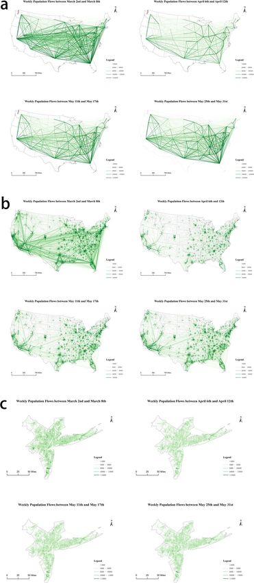
Figure 6 shows the spatial patterns of O-D flow changes during the COVID-19 pandemic based on the weekly
flow mobility data. Figure 6a,b show the spatial interaction patterns of population flows across the Contiguous
U.S. at the state and county scales, respectively. Figure 6c shows the population flow patterns at the census tract
scale in the New York metropolitan area (New York was selected as it had the most confirmed COVID-19 cases
during the study period). We take four weekly flow data to represent the spatial patterns of mobility flows before
(March 2nd to March 8th), during (April 6th to April 12th), and after (May 11th to May 17th and May 25th to
May 31st) the stay-at-home orders. At all three spatial scales, the movement flows decrease significantly from
March to April due to the stay-at-home orders, with certain increases in May with the start of state partial reo-
penings. The decrease and subsequent increase in human movement flows clearly show how the outbreak of the
COVID-19 pandemic and social distancing-related policies affect human mobility changes. In particular, accord-
ing to Fig. 6b, during the stay-at-home order period long-range spatial interactions decrease to a small quantity,
while most human movements appear as short-range movements to the adjacent counties. When cities begin to
reopen in May, long-term spatial interactions gradually rebound at both state scale and county scale.
While we made great efforts to guarantee the reliability of our produced mobility flow datasets and reduce the
data uncertainty, a few limitations should be acknowledged.
First, since we acquire anonymous mobile phone data from SafeGraph, the privacy policies applied should be
considered by the end-user, as they may influence data uncertainty. The weekly flow data is derived from CBG to
POI visitor flow metric. Please note that when a CBG has no visitors or has only one visitor who originate from
that CBG to one POI, the visit between CBG to POI will not be recorded. If the CBG has two to four visitors who
originate from that CBG to another POI, the visitor count will be recorded but shown as four to enhance differ-
ential privacy. Only when the CBG has more than five visitors whose home places inside the CBG to one POI
will the real visitor count be displayed correctly. Consequently, the least number of visitors from a CBG to POI as
well as the weekly flow data computed in one week is four. In addition, only when a visitor stays at a place (CBG
or POI) for more than one minute will a “visit” be counted. Such a relatively short time period may also affect the
foot-traffic counting and cause data uncertainty.
Second, in terms of foot-traffic counting criteria, it should be noted that, for the daily flow data, it records the
unique visitors to one CBG in one day, while for the weekly flow data it records the unique visitors to one POI
in one week. Due to the different counting methods, the sum of daily flow data in one week (i.e., seven days) are
not equal to the weekly flow data. For the daily flow data, which is computed directly based on the daily CBG to
CBG visitor flows, it may underestimate the mobility flows to POIs within one CBG. That is, a visitor may visit
more than one POI inside that CBG (e.g., different buildings in a campus) during the same day, it would still only
be recorded once from the origin CBG to the destination CBG. For the weekly flow data, which is based on the
weekly CBG to POI visitor flows, mobility flows to POIs in one week may be underestimated as a visitor may visit
one POI multiple times (e.g., work places) in one week, which would only be counted once as we compute the
unique visitor devices rather than raw visits.
In addition, visitor duplication may also exist when aggregating the flows from lower level spatial scales to
upper level spatial scales (e.g., from CBG level to census tract scale, county scale, or state scale), and it may lead
to the inflation of the inferred dynamic population flows. For example, a user may originate from his/her home
CBG and visit two POIs (e.g., one coffee shop and one grocery store) which are located inside different CBGs but
Scientific Data | (2020) 7:390 | https://doi.org/10.1038/s41597-020-00734-5 9www.nature.com/scientificdata/ www.nature.com/scientificdata
Fig. 6 Spatial patterns of mobility flows before (March 2nd to March 8th), during (April 6th to April 12th),
and after (May 11th to May 17th, May 25th to May 31st) the stay-at-home orders at three geographic scales
using weekly flow data. A: From state to state across the Contiguous U.S.; B. From county to county across the
Contiguous U.S.; C. From census tract to census tract in the New York metropolitan area. Note that the flow
dataset includes all 50 states, Washington D.C. and Puerto Rico; the flows in Hawaii, Alaska, and Puerto Rico
are not shown in the map.
at the same census tract. Such a visitor should be counted as one unique visitor from the home census tract to the
POI census tract. However, when aggregating the visits from CBG to CBG mobility flow to census tract to census
tract mobility flow, because the individual travel behaviour cannot be traced, the mobility flows between these
two census tract are counted as two and thereby inflate the real mobility flows.
Scientific Data | (2020) 7:390 | https://doi.org/10.1038/s41597-020-00734-5 10www.nature.com/scientificdata/ www.nature.com/scientificdata
Last but not least, data bias is a common issue for large-scale mobile phone data that may influence the repre-
sentativeness of our produced dataset. While dynamic mobility flows are inferred from mobile phone applications
by users, not everyone in the population has a mobile phone, and not everyone uses smartphone applications,
especially elderly people and children. Given these differences in mobile phone usage, age groups and demo-
graphic composition might influence the estimated entire population mobility flows. With these caveats in mind,
this data still provides important up-to-date mobility flow information at scale.
In conclusion, such a timely-produced dynamic O-D human flow dataset at different geographic scales can
help deepen our understanding of human dynamics under this public health crisis, inform public health policy
making, and support many other social sensing and transportation applications.
Ethical statement. An IRB review waiver certification (No. 2020-0690) was obtained from the University of
Wisconsin-Madison Education and Social/Behavioral Science institutional research board. The anonymized and
aggregated foot-traffic data that was used in the study does not involve human subjects as defined. We also follow
all the data usage agreement with SafeGraph and the university data protection policy to ensure the security of
the original data.
Code availability
Data processing and data analysis were performed on a Linux server using the Python version 3.7. All codes
used for analysis are available in the public GitHub repository that hosts the data: https://github.com/GeoDS/
COVID19USFlows.
Received: 24 June 2020; Accepted: 20 October 2020;
Published: xx xx xxxx
References
1. Dong, E., Du, H. & Gardner, L. An interactive web-based dashboard to track COVID-19 in real time. The Lancet Infectious Diseases 20,
5, 533–534 (2020).
2. Chen, S., Li, Q., Gao, S., Kang, Y. & Shi, X. Mitigating covid-19 outbreak via high testing capacity and strong transmission-
intervention in the united states. medRxiv, Preprint at https://doi.org/10.1101/2020.04.03.20052720v1 (2020).
3. Haushofer, J. & Metcalf, C. J. E. Which interventions work best in a pandemic? Science 368 6495, 1063–1065 (2020).
4. Lai, S. et al. Effect of non-pharmaceutical interventions to contain covid-19 in china. Nature (2020).
5. Askitas, N., Tatsiramos, K. & Verheyden, B. et al. Lockdown strategies, mobility patterns and covid-19. Tech. rep., Institute of Labor
Economics (IZA), 2020.
6. Gao, S. et al. Association of mobile phone location data indications of travel and stay-at-home mandates with covid-19 infection
rates in the us. JAMA Network Open 3, 9, e2020485–e2020485 (2020).
7. Wang, J., Tang, K., Feng, K. & Lv, W. When is the COVID-19 pandemic over? evidence from the stay-at-home policy execution in
106 Chinese cities. Available at SSRN: https://ssrn.com/abstract=3561491 106 (2020).
8. Chinazzi, M. et al. The effect of travel restrictions on the spread of the 2019 novel coronavirus (COVID-19) outbreak. Science (2020).
9. Liu, H. et al. Synchronized travel restrictions across cities can be effective in covid-19 control. medRxiv, Preprint at https://doi.org/
10.1101/2020.04.02.20050781v2 (2020).
10. Buckee, C. O. et al. Aggregated mobility data could help fight COVID-19. Science (New York, NY) (2020).
11. Ghader, S. et al. Observed mobility behavior data reveal social distancing inertia. arXiv preprint arXiv:2004.14748 (2020).
12. Bonato, P. et al. Mobile phone data analytics against the covid-19 epidemics in italy: flow diversity and local job markets during the
national lockdown. Preprint at arXiv:2004.11278 (2020).
13. Cintia, P. et al. The relationship between human mobility and viral transmissibility during the covid-19 epidemics in italy. Preprint
at arXiv:2006.03141 (2020).
14. Ferres, L. et al. Measuring levels of activity in a changing city: A study using cellphone data streams. Tech. rep., Instituto de Data
Science, Faculty of Engineering, UDD, April 2020.
15. Galeazzi, A. et al. Human mobility in response to covid-19 in france, italy and uk. Preprint at arXiv:2005.06341 (2020).
16. Gatto, M., Bertuzzo, E., Mari, L., Miccoli, S., Carraro, L., Casagrandi, R. & Rinaldo, A. Spread and dynamics of the covid-19 epidemic
in italy: Effects of emergency containment measures. Proceedings of the National Academy of Sciences 117, 19, 10484–10491 (2020).
17. Jia, J. S. et al. Population flow drives spatio-temporal distribution of covid-19 in China. Nature 1–5 (2020).
18. Lai, S. et al. Assessing spread risk of wuhan novel coronavirus within and beyond China, January-April 2020: a travel network-based
modelling study. medRxiv, Preprint at https://doi.org/10.1101/2020.02.04.20020479v2 (2020).
19. Li, R. et al. Substantial undocumented infection facilitates the rapid dissemination of novel coronavirus (SARS-CoV2). Science
(2020).
20. Pullano, G., Valdano, E., Scarpa, N., Rubrichi, S. & Colizza, V. Population mobility reductions during covid-19 epidemic in france
under lockdown. medRxiv. Preprint at https://doi.org/10.1101/2020.05.29.20097097v1 (2020).
21. Tian, H. et al. An investigation of transmission control measures during the first 50 days of the covid-19 epidemic in China. Science
(2020).
22. Yabe, T. et al. Non-compulsory measures sufficiently reduced human mobility in japan during the covid-19 epidemic. arXiv preprint
arXiv:2005.09423 (2020).
23. Pei, S., Kandula, S. & Shaman, J. Differential effects of intervention timing on covid-19 spread in the united states. medRxiv, Preprint
at https://doi.org/10.1101/2020.05.15.20103655v2 (2020).
24. Barbosa, H. et al. Human mobility: Models and applications. Physics Reports 734, 1–74 (2018)
25. Dong, L., Huang, Z., Zhang, J. & Liu, Y. Understanding the mesoscopic scaling patterns within cities. arXiv preprint arXiv:2001.00311
(2020).
26. Gonzalez, M. C., Hidalgo, C. A. & Barabasi, A.-L. Understanding individual human mobility patterns. Nature 453, 7196, 779–782
(2008).
27. Boarnet, M. G., Hong, A. & Santiago-Bartolomei, R. Urban spatial structure, employment subcenters, and freight travel. Journal of
Transport Geography 60, 267–276 (2017).
28. Li, B. et al. Estimation of regional economic development indicator from transportation network analytics. Scientific Reports 10, 1,
1–15 (2020).
29. Hincks, S. & Wong, C. The spatial interaction of housing and labour markets: commuting flow analysis of north west england. Urban
Studies 47, 3, 620–649 (2010).
Scientific Data | (2020) 7:390 | https://doi.org/10.1038/s41597-020-00734-5 11www.nature.com/scientificdata/ www.nature.com/scientificdata
30. Jia, C., Du, Y., Wang, S., Bai, T. & Fei, T. Measuring the vibrancy of urban neighborhoods using mobile phone data with an improved
pagerank algorithm. Transactions in GIS 23, 2, 241–258 (2019).
31. Tu, W. et al. Coupling mobile phone and social media data: A new approach to understanding urban functions and diurnal patterns.
International Journal of Geographical Information Science 31, 12, 2331–2358 (2017).
32. Li, M., Shi, X. & Li, X. Integration of spatialization and individualization: the future of epidemic modelling for communicable
diseases. Annals of GIS, 1–8 (2020).
33. Gao, S., Liu, Y., Wang, Y. & Ma, X. Discovering spatial interaction communities from mobile phone data. Transactions in GIS 17, 3,
463–481 (2013).
34. Liu, Y., Sui, Z., Kang, C. & Gao, Y. Uncovering patterns of inter-urban trip and spatial interaction from social media check-in data.
PloS One 9, 1 (2014).
35. Ratti, C., Frenchman, D., Pulselli, R. M. & Williams, S. Mobile landscapes: using location data from cell phones for urban analysis.
Environment and planning B: Planning and design 33, 5, 727–748 (2006).
36. Franch-Pardo, I., Napoletano, B. M., Rosete-Verges, F. & Billa, L. Spatial analysis and gis in the study of covid-19. a review. Science of
The Total Environment 140033 (2020).
37. Gao, S., Rao, J., Kang, Y., Liang, Y. & Kruse, J. Mapping county-level mobility pattern changes in the united states in response to
covid-19. SIGSPATIAL Special 12, 1, 16–26 (2020).
38. Oliver, N. et al. Mobile phone data for informing public health actions across the covid-19 pandemic life cycle. Science Advances 23
6, eabc0764 (2020).
39. Warren, M. S. & Skillman, S. W. Mobility changes in response to COVID-19. arXiv preprint arXiv:2003.14228 (2020).
40. Aktay, A. et al. Google COVID-19 community mobility reports: Anonymization process description (version 1.0). Preprint at
arXiv:2004.04145 (2020).
41. Kuchler, T., Russel, D. & Stroebel, J. The geographic spread of covid-19 correlates with structure of social networks as measured by
facebook. Tech. rep., National Bureau of Economic Research, 2020.
42. Holtz, D. et al. Interdependence and the cost of uncoordinated responses to COVID-19. Proceedings of the National Academy of
Sciences 117, 33, 19837–19843 (2020).
43. Kraemer, M. U. et al. The effect of human mobility and control measures on the COVID-19 epidemic in China. Science (2020).
44. Wilkinson, M. D. et al. The fair guiding principles for scientific data management and stewardship. Scientific Data 3 (2016).
45. Pepe, E. et al. Covid-19 outbreak response, a dataset to assess mobility changes in italy following national lockdown. Scientific Data
7 1, 1–7 (2020).
46. SafeGraph. The impact of coronavirus (COVID-19) on foot traffic, https://www.safegraph.com/dashboard/covid19-commerce-
patterns (2020).
47. Huang, Q. & Xiao, Y. Geographic situational awareness: mining tweets for disaster preparedness, emergency response, impact, and
recovery. ISPRS International Journal of Geo-Information 4, 3, 1549–1568 (2015).
48. Song, X., Zhang, Q., Sekimoto, Y. & Shibasaki, R. Prediction of human emergency behavior and their mobility following large-scale
disaster. In Proceedings of the 20th ACM SIGKDD international conference on Knowledge discovery and data mining, pp. 5–14 (2014).
49. Bassolas, A. et al. Hierarchical organization of urban mobility and its connection with city livability. Nature Communications 10, 1,
1–10 (2019).
50. Hatton, T. J., Williamson, J. G. et al. Global migration and the world economy: Two centuries of policy and performance. MIT press
Cambridge, MA, 2005.
51. SafeGraph. What about bias in the SafeGraph dataset?, available at https://www.safegraph.com/blog/what-about-bias-in-the-
safegraph-dataset (2020).
52. SafeGraph. Common Nighttime Location Algorithm, available at https://docs.safegraph.com/docs/places-manual#section-safe-
graph-common-nighttime-location-algorithm (2020).
53. Ester, M., Kriegel, H.-P., Sander, J. & Xu, X. Density-based spatial clustering of applications with noise. In Int. Conf. Knowledge
Discovery and Data Mining, vol. 240, p. 6 (1996).
54. SafeGraph. Determining Point-of-Interest Visits From Location Data: A Technical Guide To Visit Attribution,COVID-19 Datasets,
available at https://www.safegraph.com/visit-attribution (2020).
55. Atkinson, P. M. & Tate, N. J. Spatial scale problems and geostatistical solutions: a review. The Professional Geographer 52, 4, 607–623
(2000).
56. Chen, L., Gao, Y., Di Zhu, Y. Y. & Liu, Y. Quantifying the scale effect in geospatial big data using semi-variograms. PloS One 14, 11
(2019).
57. Liu, Y., Kang, C., Gao, S., Xiao, Y. & Tian, Y. Understanding intra-urban trip patterns from taxi trajectory data. Journal of
Geographical Systems 14, 4, 463–483 (2012).
58. Andris, C. Integrating social network data into gisystems. International Journal of Geographical Information Science 30, 10,
2009–2031 (2016).
59. Benach, J., Muntaner, C., Delclos, C., Menéndez, M. & Ronquillo, C. Migration and low-skilled workers in destination countries.
PLoS Medicine 8, 6, e1001043 (2011).
60. Fiorio, L. et al. Using twitter data to estimate the relationship between short-term mobility and long-term migration. In Proceedings
of the 2017 ACM on web science conference, pp. 103–110 (2017).
61. Prieto Curiel, R., Pappalardo, L., Gabrielli, L. & Bishop, S. R. Gravity and scaling laws of city to city migration. PloS One 13, 7,
e0199892 (2018).
62. Yeghikyan, G., Opolka, F. L., Nanni, M., Lepri, B. I Lio, P. Learning mobility flows from urban features with spatial interaction
models and neural networks. Preprint at arXiv:2004.11924 (2020).
63. Kang, Y. et al. Multiscale dynamic human mobility flow dataset in the U.S. during the COVID-19 epidemic. figshare https://doi.
org/10.6084/m9.figshare.c.5032634.v1 (2020).
64. US Census Bureau. Understanding Geographic Identifiers (GEOIDs), https://www.census.gov/programs-surveys/geography/
guidance/geo-identifiers.html (2020).
65. Kang, C., Liu, Y., Guo, D. & Qin, K. A generalized radiation model for human mobility: spatial scale, searching direction and trip
constraint. PloS One 10, 11, e0143500 (2015).
66. Simini, F., González, M. C., Maritan, A. & Barabási, A.-L. A universal model for mobility and migration patterns. Nature 484, 7392,
96–100 (2012).
67. Killeen, B. D. et al. A county-level dataset for informing the united states’ response to covid-19. arXiv preprint arXiv:2004.00756
(2020).
68. O’Kelly, M. E., Song, W. & Shen, G. New estimates of gravitational attraction by linear programming. Geographical Analysis 27, 4,
271–285 (1995).
69. Eberhart, R. & Kennedy, J. A new optimizer using particle swarm theory. In MHS’95. Proceedings of the Sixth International
Symposium on Micro Machine and Human Science, IEEE, pp. 39–43 (1995).
70. Liang, Y., Gao, S., Cai, Y., Foutz, N. Z. & Wu, L. Calibrating the dynamic huff model for business analysis using location big data.
Transactions in GIS 24, 3, 681–703 (2020).
71. US Census Bureau. American Community Survey (ACS) commuting flows, https://www.census.gov/topics/employment/
commuting/guidance/flows.html (2020).
Scientific Data | (2020) 7:390 | https://doi.org/10.1038/s41597-020-00734-5 12You can also read