Correcting Bias in Crowdsourced Data to Map Bicycle Ridership of All Bicyclists - MDPI
←
→
Page content transcription
If your browser does not render page correctly, please read the page content below
Article
Correcting Bias in Crowdsourced Data to Map Bicycle
Ridership of All Bicyclists
Avipsa Roy 1, * , Trisalyn A. Nelson 1 , A. Stewart Fotheringham 1 and Meghan Winters 2
 1    School of Geographical Sciences and Urban Planning, Arizona State University, 975 S Myrtle Ave,
      COOR Hall, 5th Floor, Tempe, AZ 85281, USA; Trisalyn.Nelson@asu.edu (T.A.N.);
      Stewart.Fotheringham@asu.edu (A.S.F.)
 2    Faculty of Health Sciences, Simon Fraser University, Blusson Hall, 8888 University Drive,
      Burnaby, BC V5A 1S6, Canada; meghan_winters@sfu.ca
 *    Correspondence: aroy29@asu.edu or Avipsa.Roy@asu.edu

 Received: 21 April 2019; Accepted: 29 May 2019; Published: 4 June 2019

 Abstract: Traditional methods of counting bicyclists are resource-intensive and generate data with
 sparse spatial and temporal detail. Previous research suggests big data from crowdsourced fitness
 apps offer a new source of bicycling data with high spatial and temporal resolution. However,
 crowdsourced bicycling data are biased as they oversample recreational riders. Our goals are to
 quantify geographical variables, which can help in correcting bias in crowdsourced, data and to
 develop a generalized method to correct bias in big crowdsourced data on bicycle ridership in different
 settings in order to generate maps for cities representative of all bicyclists at a street-level spatial
 resolution. We used street-level ridership data for 2016 from a crowdsourced fitness app (Strava),
 geographical covariate data, and official counts from 44 locations across Maricopa County, Arizona,
 USA (training data); and 60 locations from the city of Tempe, within Maricopa (test data). First,
 we quantified the relationship between Strava and official ridership data volumes. Second, we used a
 multi-step approach with variable selection using LASSO followed by Poisson regression to integrate
 geographical covariates, Strava, and training data to correct bias. Finally, we predicted bias-corrected
 average annual daily bicyclist counts for Tempe and evaluated the model’s accuracy using the test
 data. We found a correlation between the annual ridership data from Strava and official counts (R2 =
 0.76) in Maricopa County for 2016. The significant variables for correcting bias were: The proportion
 of white population, median household income, traffic speed, distance to residential areas, and
 distance to green spaces. The model could correct bias in crowdsourced data from Strava in Tempe
 with 86% of road segments being predicted within a margin of ±100 average annual bicyclists. Our
 results indicate that it is possible to map ridership for cities at the street-level by correcting bias in
 crowdsourced bicycle ridership data, with access to adequate data from official count programs and
 geographical covariates at a comparable spatial and temporal resolution.

 Keywords: bias correction; LASSO; active transportation; big data; crowdsourcing

1. Introduction
     Lack of physical activity is identified as one of the primary factors leading to increased risk
of chronic diseases, including obesity, cardiovascular diseases [1], and type 2 diabetes [2] as well
as cancer [3]. The World Health Organization recommends a minimum of 150 min of moderate
physical activity per week [4]. Active transportation modes (bicycling and walking) help to incorporate
routine physical activity among adults with a sedentary lifestyle to reduce health risks. Consequently,
public health and urban planning agencies are increasingly recognizing the importance of active
transportation [5] in their pursuit of broader public health goals [6], creating a demand for a better

Urban Sci. 2019, 3, 62; doi:10.3390/urbansci3020062                             www.mdpi.com/journal/urbansci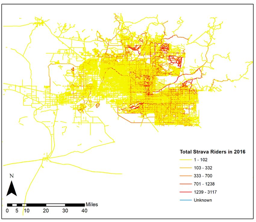
Urban Sci. 2019, 3, 62                                                                               2 of 20

 understanding of the influences on bicycle ridership. Previous studies [7,8] have used empirical
 methods to inform policymakers about necessary infrastructure changes using origin-destination
 surveys to help increase physical activity levels among adults.
       Unfortunately, there are large gaps in the data resolution, coverage, and quality for active
 transportation at the street segment level. Existing approaches to bicycle counting result in data with
poor spatial detail and/or limited temporal coverage [9]. The three most common ways to collect
 bicycle ridership data are manual counts [10], temporary, and continuous counters [9]. Manual counts,
 often conducted by volunteers, typically enumerate the number of cyclists at major street intersections
 during peak commuting periods for a few days of the year [11], and lack dense spatial coverage and
 temporal detail [12]. Temporary counts (i.e., tube counters set out for a week or two) provide a snapshot
 of ridership at a location over time, but, typically, the spatial coverage is limited. Automated counters
(counting bicyclists crossing a specific street intersection continuously) [13] have great temporal detail,
 but often lack spatial coverage.
       Crowdsourcing has, therefore, emerged as a tool of interest for collecting data on bicycling
 ridership [14–16], comfort mapping for bicyclists [17], understanding the effects of the built environment
 on ridership [18], and promoting safety among riders [19]. The emergence of crowdsourced data
 generated by fitness apps (e.g., Strava.com) has provided a new source of ridership data with enhanced
 spatial and temporal resolutions [20]. With the proliferation of smartphones, fitness apps, such as
 Strava, have emerged as one of the most popular and rich sources of data for physical activity tracking;
 Strava records an average of 2.5 million GPS routes weekly by users across 125 cities all over the
world [21].
       However, the primary concern with crowdsourced data is the bias towards recreational riders,
who are frequent users of GPS-enabled fitness apps. Thus, there is a need to quantify and correct
 the inherent bias in crowdsourced data [22] for a better representation of the ridership patterns of
 all riders, across varying ages and abilities. A generalized bias correction approach across all spatial
 and temporal scales is desirable to facilitate mainstream usage of crowdsourced fitness app data from
platforms, such as Strava, for public health and urban planning. Most studies on bias in crowdsourced
 data [23] focus on characterizing the nature of the bias [24,25]. We hypothesize that crowdsourced data
 in urban settings can be used to map bicycling ridership [20,26]. Here, we move the research forward
 by developing a generalized approach to bias correction that combines traditionally collected ridership
 data with crowdsourced data to fill gaps in the spatial and temporal detail.
       Our goal is twofold—first, to quantify which geographical variables can help in correcting bias in
 crowdsourced data; and second, to develop a generalized method to correct bias in big crowdsourced
 data on bicycle ridership in different settings to generate maps representative of all bicyclists at a
 street-level spatial resolution. Maps were created with enhanced spatial and temporal detail given the
‘big data’ provided by crowdsourced fitness apps. Bias correction was framed as using crowdsourced
 fitness app user counts along with additional geographic covariates to predict average annual daily
 bicyclist (AADB) counts on a street network. The result is a map that shows the ridership of bicyclists
 of all ages and abilities, even those that do not use the app.

2. Materials and Methods

2.1. Study Area
     Our study area was the Maricopa County in the state of Arizona, USA, and covers 9200 square
miles (Figure 1). Maricopa County includes 27 cities anchored by Phoenix [27]. With a population of
over 3.3 million people, it is the fourth most populous county in the USA [28]. The weather is mostly
arid with summer temperatures ranging from 50 ◦ F (10 ◦ C) to 108 ◦ F (42 ◦ C) and winter temperatures
between 35 ◦ F (1 ◦ C) and 90 ◦ F (26 ◦ C), with an average precipitation of 132 mm in summer and
236 mm in winter. The city of Tempe, within Maricopa County, specifically has more than 175 miles of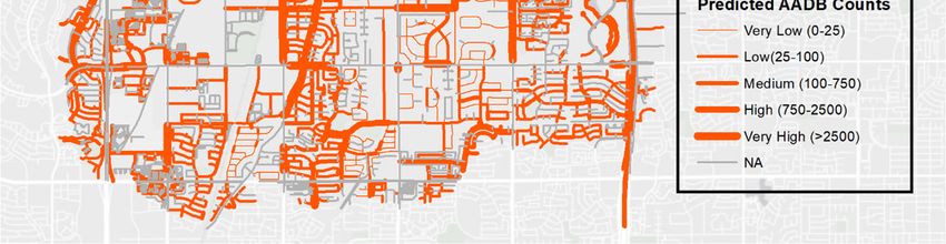
Urban Sci. 2019, 3, 62                                                                                        3 of 20

bikeways and the highest percentage of residents commuting by means of bicycles at 4.2%, far higher
than the Maricopa County average of 0.8% [29].
 Urban Sci. 2019, 3, x FOR PEER REVIEW                                                        3 of 19

                                Figure1.1.Study
                               Figure      Studyarea
                                                 areaininMaricopa
                                                         MaricopaCounty,
                                                                  County,AZ,
                                                                          AZ,USA.
                                                                              USA.

2.2.
 2.2.Data
     DataSources
          Sources

2.2.1.
 2.2.1.Official
       OfficialBicycle
                BicycleCounts
                        Counts
     Two
      Twoofficial
            officialcount
                     countdata
                            datasets
                                 setswere
                                      wereused,
                                             used,thethefirst
                                                          firsttototrain
                                                                    trainthe
                                                                           themodel
                                                                                modeland andthe
                                                                                             thesecond
                                                                                                  secondtototest
                                                                                                             testthe
                                                                                                                  the
model.  To train  the model, we  used  temporary,     automated      bicycle  counts  completed
 model. To train the model, we used temporary, automated bicycle counts completed by the Maricopa  by the Maricopa
Association
 AssociationofofGovernments
                   Governments (MAG)
                                  (MAG)at 44atlocations  in 2016
                                                44 locations     in(Figure   2). We used
                                                                     2016 (Figure          the used
                                                                                      2). We   commonly    reported
                                                                                                     the commonly
time period, the  annual  average daily  bicyclist  (AADB)     count,   for the official counts
 reported time period, the annual average daily bicyclist (AADB) count, for the official counts as provided   by theas
MAG.   Bicyclists
 provided   by the were counted
                      MAG.        by thewere
                             Bicyclists   MAGcounted
                                                  using automated
                                                             by the MAG  counters   with
                                                                                using      pneumaticcounters
                                                                                         automated     tubes over  a
                                                                                                                 with
span of eight  continuous   two-week   periods    in the  months     of  April, May,   October,
 pneumatic tubes over a span of eight continuous two-week periods in the months of April, May,   and  November    to
understand
 October, andand   capture the
                November    to variation
                               understand in seasonal
                                             and capturecycling    volumes. in seasonal cycling volumes.
                                                             the variation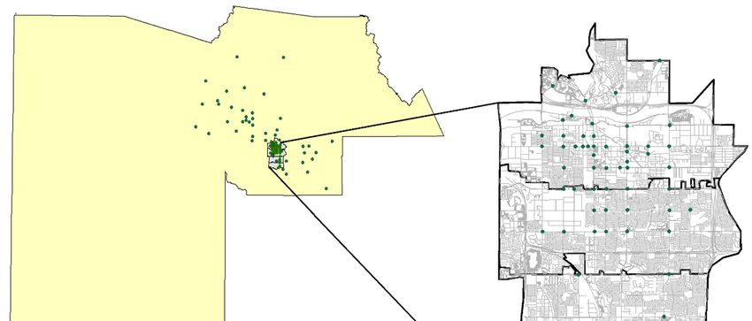
Urban Sci. 2019, 3, 62 4 of 20
Urban Sci. 2019, 3, x FOR PEER REVIEW 4 of 19
Figure 2.
Figure Average annual
2. Average annual daily bicyclist counts in Maricopa County in 2016.
The count
The count locations
locations covered
covered the
the most
most populated
populated regions
regions within
within Maricopa
Maricopa County
County andand spanned
spanned
12 major
12 major cities, including Avondale,
cities, including Avondale, Carefree,
Carefree, Chandler,
Chandler, Gilbert,
Gilbert, Glendale,
Glendale, Litchfield
Litchfield Park,
Park, Mesa,
Mesa,
Peoria, Phoenix, Queen Creek, Scottsdale, and Tempe. Figure 2 shows the AADB
Peoria, Phoenix, Queen Creek, Scottsdale, and Tempe. Figure 2 shows the AADB counts in order counts in order of the
of
population
the density
population of each
density citycity
of each within Maricopa
within MaricopaCounty.
County.TheThe
counters
counters were
werelocated
locatedacross
acrossa range
a rangeof
locations, including freeways and arterials with and without bike facilities, as well as
of locations, including freeways and arterials with and without bike facilities, as well as bike paths, bike paths, such
as near
such as canals and trails.
near canals The AADB
and trails. countscounts
The AADB were extrapolated based upon
were extrapolated basedtheupon2-week period counts.
the 2-week period
Also, owing
counts. Also,toowing
the extreme
to the weather
extreme conditions, overall ridership
weather conditions, is generally
overall ridership is lower in the
generally study
lower inarea
the
compared to other North American cities.
study area compared to other North American cities.
We used
We used anan independent
independent testtest dataset
dataset to
to evaluate
evaluate the
the model
model prediction
prediction accuracy,
accuracy, from
from thethe city
city of
of
Tempe, where
Tempe, where manual
manual bicyclist
bicyclist counts
counts across
across 60
60 locations
locations were
were available. These manual
available. These manual counts
counts werewere
conducted by a non-profit organization, the Tempe Bicycle Action Group (TBAG),
conducted by a non-profit organization, the Tempe Bicycle Action Group (TBAG), at peak periods in at peak periods in
the morning
the morning (0700–0900)
(0700–0900) and and evening
evening (1600–1800)
(1600–1800) onon weekdays
weekdays in in the
the months
months of of April
April toto May
May andand
October to November in 2016, and 12,345 cyclists were recorded. The bicycle ridership
October to November in 2016, and 12,345 cyclists were recorded. The bicycle ridership data collected data collected
by the
by the TBAG
TBAG werewereused
usedtotoevaluate
evaluatethe
theglobal
globalmodel
model accuracy at aatsmaller
accuracy a smallerspatial scale,
spatial justjust
scale, for the
for city
the
of Tempe.
city of Tempe.
2.2.2. Crowdsourced
2.2.2. Crowdsourced Data
Data from
from Fitness
Fitness App
App
The Maricopa
The MaricopaAssociation
AssociationofofGovernments
Governments distributed
distributedStrava bicycling
Strava datadata
bicycling for 2016
for for
2016thefor
entire
the
Maricopa
entire County.
Maricopa StravaStrava
County. data included street network
data included shapefiles
street network with anonymized
shapefiles with anonymized bicyclist count
bicyclist
information
count along with
information alongeach
withstreet
eachsegment as well as
street segment as at street
well intersections,
as at at a one-minute
street intersections, temporal
at a one-minute
resolution.resolution.
temporal The high spatial
The highandspatial
temporal
andcoverage
temporalofcoverage
the Stravaof data in Maricopa
the Strava data inCounty
Maricopaallowed
Countyfor
counts to be obtained in the same locations and time periods as those collected through
allowed for counts to be obtained in the same locations and time periods as those collected through automated
count stations.
automated The
count total number
stations. ofnumber
The total Strava riders throughout
of Strava Maricopa Maricopa
riders throughout County inCounty
2016 is in
shown
2016 in
is
Figure 3.
shown in Figure 3.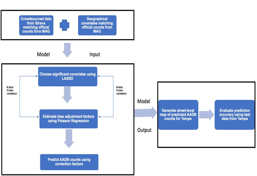
Urban Sci. 2019, 3, 62                                                                                     5 of 20
 Urban Sci. 2019, 3, x FOR PEER REVIEW                                                                   5 of 19
  Urban Sci. 2019, 3, x FOR PEER REVIEW                                                                  5 of 19

                       Figure
                        Figure3. Distribution  of Strava riders in Maricopa County
                                                                            County for2016.
                                                                                       2016.
                        Figure 3.
                               3. Distribution
                                  Distribution of
                                               of Strava
                                                  Strava riders in Maricopa
                                                                   Maricopa County for
                                                                                   for 2016.

      Among
       Among   all the Strava riders,  nearly 76.5%    of Strava riders in 2016 in Maricopa    County werewere
                                                                                                             male,
        Among allall the
                     the Strava
                          Strava riders,
                                  riders, nearly
                                          nearly 76.5%
                                                  76.5% ofof Strava
                                                             Strava riders
                                                                    riders in
                                                                            in 2016
                                                                               2016 in
                                                                                     in Maricopa
                                                                                        Maricopa County
                                                                                                   County were
17.6%
  male,were female,     and 5.9% did    not specify   a gender, as shown    in FigureFigure
                                                                                       4, whichwhich
                                                                                                 indicates Strava
  male, 17.6%
         17.6% were
                 were female,
                        female, and
                                 and 5.9%
                                     5.9% did
                                           did not
                                                not specify
                                                    specify aa gender,
                                                               gender, as
                                                                        as shown
                                                                           shown inin Figure 4,
                                                                                              4, which indicates
                                                                                                        indicates
riders
  Stravawere  notwere
                    fully representative    of the of
                                                   entire  population   and there   waswasan inherent  bias in in
                                                                                                               the
  Strava riders were not fully representative of the entire population and there was an inherent bias
          riders        not fully representative      the entire population   and there       an inherent bias in
ridership
  the       data,
  the ridership   which
      ridership data,     requires
                  data, which       correction.
                         which requires
                                requires correction.
                                          correction.

                 Figure
                 Figure4.4. Age–gender
                         4.Age–gender  distribution
                            Age–genderdistribution  of
                                       distribution of Strava
                                                       Strava riders
                                                    of Strava riders in
                                                                     in Maricopa County for 2016.
                Figure                                        riders in Maricopa
                                                                        Maricopa County
                                                                                 Countyfor
                                                                                         for2016.
                                                                                             2016.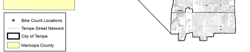
Urban Sci. 2019, 3, 62                                                                                                    6 of 20

2.2.3. Explanatory Geographical Covariates
     In Table 1, we list the explanatory geographical covariates used in our model along with their
potential relationship with bicycling. The geographical covariates were provided by the MAG for
each census block group in Maricopa County. We identified those census block groups which were
intersected by a unique street segment and assigned the mean of all the variables in the intersected
polygons to the respective street segment. We also used the shortest distance technique to compute the
proximity to green spaces, residential areas, and commercial areas for each individual street segment.
The shortest distance is the Euclidean or straight-line distance from the nearest land-use polygon of a
specific type (e.g., green space/residential area/commercial area) to the street segment. The MAG also
provided the shapefiles on land-use classes, which were used to categorize green spaces, residential,
and commercial areas.

                  Table 1. Geographical covariates influencing ridership in Maricopa County (2016).

        Description             Measure                    Source         Year   Resolution            Relevance
                         Bicyclist count across                                               Crowdsourced cycling data
       Crowdsourced      street segments                                         Street       help predict categories of
                                                   Strava Metro           2016
       Fitness App       grouped by location                                     Segment      cycling volumes in urban
                         and timestamp                                                        environments [15,20].
                                                                                              Built environment has a
                         (a)   Average daily       (a)   USDOT Federal                        significant influence on
       Built                   traffic volume            Highways                Street       active transportation choices
                         (b)   Average segment           Administration   2016
       Environment                                                               Segment      [1,18,30,31].
                               speed limit         (b)   OpenStreetMap                        Improving traffic promotes
                                                                                              bicycling [32].

                         (a)
                               Population density
                         (b)   %                                                              Densely populated areas
                                                                                 AZ
                               white population Maricopa Association             Census
                                                                                              have higher number of
       Demographics      (c)   Median age         of Governments Open     2010                cyclists [33,34].
                                                                                 Block
                         (d)   % veterans         Data Portal                                 Ethnicity variations affect
                                                                                 Group
                                                                                              bicycle ridership levels [35].
                         (e)   % high
                               school educated

                         (a)   Proximity
                               to greenspace                                                  Nearness to residential areas
                         (b)   Proximity to        Maricopa Association                       and green open spaces has
                                                                                 Street
       Land Use Mix            residential areas   of Governments Land    2016                shown positive associations
                                                                                 Segment
                         (c)   Proximity to        Use Data                                   with an increase in physical
                               commercial areas                                               activity [1,36].

                                                                                 AZ
                         (a)   Median              Maricopa Association                       Areas with lower income
                                                                                 Census
       Socio-Economic          household income    of Governments Open    2010                levels tend to bike more
                                                                                 Block
                                                   Data Portal                                [10,37,38].
                                                                                 Group

                         (a)   % of population                                   AZ           Frequent bicycle commuters
                               who commute to      Maricopa Association
       Commute                                                                   Census       are more likely to have a
                               work                of Governments Open    2010
       Patterns                                                                  Block        higher level of education
                               with bicycles       Data Portal
                                                                                 Group        [39].

2.3. Model Design and Analysis
    Our approach for bias correction employed a multi-step approach as shown in Figure 5.
We performed the following steps for correcting bias in the Strava data:
(i)     The relationship between the Strava ridership data and official counts across 44 locations in
        Maricopa County (train data) was quantified using ordinary least squares regression.
(ii)    Additional geographic data from multiple disparate sources (Table 1) were then aligned,
        controlling for variable multicollinearity, with ridership data from Strava, and a variable selection
Urban Sci. 2019, 3, 62 7 of 20
technique—LASSO—was used to identify the most significant geographical variables from all the
listedSci.variables
Urban in PEER
2019, 3, x FOR TableREVIEW
1. 7 of 19
(iii) A generalized linear model with a Poisson distribution was fitted using the observed AADB counts
(iii)
as a A generalizedvariable
dependent linear model
and thewith a Poisson
Strava distribution
ridership was fitted
data along withusing the observed AADB
the geographical covariates
counts as a dependent variable and the Strava ridership data along
selected by LASSO, which were outcomes of step (ii), at comparable spatial and temporal scales with the geographical
covariates selected by LASSO, which were outcomes of step (ii), at comparable spatial and
as independent variables. Using this model, we corrected the bias in the crowdsourced bicycle
temporal scales as independent variables. Using this model, we corrected the bias in the
ridership data by age and ability across Maricopa County using a 10-fold cross-validation across
crowdsourced bicycle ridership data by age and ability across Maricopa County using a 10-fold
the 44 locations. across the 44 locations.
cross-validation
(iv) (iv)
The The
coefficients of of
coefficients thethe
model
modelfitted
fittedinin step
step (iii) werethen
(iii) were thenused
used to to explain
explain the the variation
variation in thein the
AADB AADB counts
countsandand
thethe
bias-corrected
bias-correctedpredictions.
predictions.
(v) (v)
The The best-fitted
best-fitted model
model fromstep
from step(iii)
(iii)was
was cross-validated,
cross-validated, which
which is aistechnique
a technique usedused
to test
to the
test the
model fit by holding out 10% of the data and training the model with 90%
model fit by holding out 10% of the data and training the model with 90% of the data in multiple of the data in multiple
iterations, and the model with least cross-validation error was used to predict the observed
iterations, and the model with least cross-validation error was used to predict the observed AADB
AADB at unknown locations and to create a street-level map of bias-corrected AADB counts in
at unknown locations and to create a street-level map of bias-corrected AADB counts in Tempe.
Tempe.
(vi) (vi)
Finally, the prediction
Finally, the prediction accuracy
accuracyofofthe
themodel, shownininstep
model, shown step(iii),
(iii), was
was evaluated
evaluated in Tempe
in Tempe across across
60 locations
60 locationswherewhereground
ground truth
truthdata
datafor
for the
the AADB countswere
AADB counts were available
available (test
(test data).
data).
Figure
Figure 5. Model
5. Model design
design forbicycle
for bicycleridership
ridership prediction
predictionusing
usingPoisson regression.
Poisson regression.
EachEach of the
of the steps
steps is explainedininfurther
is explained further detail
detail in
in the
thesections
sectionsthat follow.
that TheThe
follow. exploratory
exploratory
analysis and data preprocessing were performed using Jupyter Notebooks [40]. Spatial analyses were
analysis and data preprocessing were performed using Jupyter Notebooks [40]. Spatial analyses
undertaken in ESRI® ArcGIS 9.3 and the model was partly built using both Python 3.5 [41] and R 3.4
were undertaken in ESRI® ArcGIS 9.3 and the model was partly built using both Python 3.5 [41] and
[42].
R 3.4 [42]. For more details on the code used in the steps (i) to (vi), please refer the Supplementary
Materials.
2.3.1. Comparison of Official and Crowdsourced Bicyclist Counts
To quantify
2.3.1. Comparison ofhow the bicycle
Official ridership of all riders
and Crowdsourced is represented
Bicyclist Counts by sampling the crowdsourced
app ridership, we compared the ridership counts from Strava with official counts from automated
To quantify
bike counter how theinstalled
systems bicycle ridership
by the MAG of all
[27]riders
acrossis44represented
locations in by sampling
Maricopa the crowdsourced
County for a two-
week period
app ridership, weincompared
the months theofridership
April, May, October,
counts fromand November.
Strava The Python
with official countspackage, PANDAS bike
from automated
(Python
counter systemsdata installed
analysis library)
by the [43],
MAG was used
[27] to summarize,
across 44 locationsmatch, and extractCounty
in Maricopa crowdsourced data
for a two-week
counts
period in theformonths
each individual
of April,road
May, segment in Maricopa
October, County to
and November. Theaccount forpackage,
Python ridership PANDAS
estimates. (PythonUrban Sci. 2019, 3, 62 8 of 20
data analysis library) [43], was used to summarize, match, and extract crowdsourced data counts for
each individual road segment in Maricopa County to account for ridership estimates.
Comparisons between the two datasets were made at daily, monthly, and annual levels. We used
regression analysis to quantify how much of the variation in bicycle ridership was explained by the
crowdsourced data. To do this, we matched counts from Strava, aggregated into hourly intervals,
and matched those to the time windows when official counts were conducted by the MAG. Once
counts were matched temporally, we compared both datasets at daily, monthly, and annual levels.
We obtained R2 values using simple linear regression for each time period and retained the volumes
with the highest R2 for further analyses.
2.3.2. Variable Selection for Bias Correction Using LASSO
In order to correct for the bias in the crowdsourced ridership data, we included the geographical
covariates from Table 1. Variable multicollinearity, which is the state of high inter-correlations among
independent variables, was limited by retaining only those variables which had a variance inflation
factor (VIF) below 7.5 [44]. If the variance inflation factor of a predictor variable was 7.5, this meant that
√
the standard error for the coefficient of that predictor variable was 2.73 ( 7.5) times as large as it would
be if that predictor variable was uncorrelated with the other predictor variables. These covariates were
hypothesized to influence bicycle ridership at a geographic scale comparable to that of the Strava data.
Spatial joins from the Python library, Geopandas [45], were used to link bicycling counts data with the
geographical covariates.
We used an average of the geographical covariates for all the census block groups that a particular
street segment intersected. The distance variables were calculated in ArcGIS using a simple Euclidean
distance measured in miles. Since the number of independent variables for our analysis was 15, even
after accounting for inter-correlations through VIF, we used a statistical method to select only those
variables that explained most of the variance in the overall bicycle ridership. A variable selection
technique using LASSO (least absolute shrinkage and selection operator) [46] was applied to select
covariates that best explained the bias in the Strava data, while accounting for the bias–variance the
tradeoff [46].
The purpose of LASSO is to apply a constraint on the sum of the absolute values of the model
parameters with a fixed upper bound. To do so, the method applies a shrinkage process (also known
as regularization), where it penalizes the coefficients of the independent variables, shrinking some of
them to zero. The variables that still have a non-zero coefficient after the shrinkage were selected to be
inputs of the final Poisson regression model. By using LASSO, we intended to minimize the prediction
error of the final AADB counts. The LASSO can be thought of as an additional step, which can help
transportation planners choose, from a large set of variables in a study area, only those which can in
effect help improve the prediction results and contribute significantly in explaining variation in the
overall bicycle ridership.
Given the set of explanatory variables, x1 , x2 . . . xp , and the outcome, y, the observed bike counts,
LASSO fits the linear model:
ŷ = β0 + β1 .x1 + . . . . . . . + βp .xp (i), (1)
by minimizing the following criterion:
Xn Xp
( y − ŷ)2 + λ βj . (2)
i=1 j=1
In doing so, the non-contributing geographical covariates are shrunk to zero. We ran 200 iterations
of the LASSO on our training data using a 10-fold cross-validation approach to obtain the optimal value
for λ (tuning parameter), which yielded the minimum cross-validation error on the training dataset for
all iterations. The variable selection was performed using the randomized LASSO scores provided byUrban Sci. 2019, 3, 62 9 of 20
the scikit-learn Python library based on the stability function proposed by [47]. For a cut-off, πi , with 0
< πi < 1 and a set of regularization parameters, Λ, the set of stable variables is defined as:
λ̂
Y
Ŝstable = {k : max( ) ≥ πi }. (3)
k
With the chosen λ, we retained the variables with a high selection probability and disregarded those
with low selection probabilities using a score function, which provided the coefficient of determination,
R2 , of the prediction ranging from 0 to 1. The coefficient, R2 , is defined as (1 − u/v), where u is the
residual sum of squares and v is the total sum of squares of the variables retained with the chosen
value of λ. The LASSO module from the Python machine learning library, scikit-learn, was used to
perform variable selection.
2.3.3. Estimating Bias-Corrected Bicycle Volumes from a Crowdsourced Fitness App and
Geographical Covariates
We fitted the geographical covariates selected by LASSO to a generalized linear model following
a Poisson distribution to explore the relationships among the selected covariates, and the bicycle
ridership counts in Maricopa County using Equation (3). We chose the Poisson model as it generates
non-negative predictions, which are appropriate for modeling count data.
As shown in Figure 2, the geographical variables as well as the official counts and counts from the
crowdsourced app were provided as inputs to the model. The LASSO variable selection algorithm
determined the stable covariates that best replicate the bicyclist counts. Following variable selection, the
Poisson model predicted the AADB counts along all street segments in Maricopa County. The regression
model was specified as a Poisson distribution with a log-link function [48] as follows:
Yi ∼ Poisson(µi ), log(µi ) = βi Xi , (4)
where:
Yi = the AADB counts at site i
βi = vector of parameters for count site i
Xi = vector of the observed geographical covariates for count site i.
The AADB counts were generated by the model across the entire road network in Maricopa
County, including paved streets with and without bike facilities. The segments from Strava that were
matched in spatial and temporal resolution to the official MAG counts were used in fitting the Poisson
model. Hence, we could compare the counts from both sources at only those locations, where both
counts were available, which were then used to train our model. The remaining segments that only
had Strava counts were used to test the predictive power of the model. The average annual counts
from Strava along with the geographical covariates were the independent variables for the model.
The significant variables were those with a p-value < 0.001. Since we assumed that our dependent
variables (the MAG counts) follow a Poisson distribution with a mean that depends on some covariates,
we used a generalized linear model that takes into account the heteroscedasticity in the data.
2.3.4. Predicting Ridership Using Poisson Model Coefficients
The Poisson model coefficients were used to predict ridership at all street segments in Tempe.
A k-fold cross-validation technique [49] was used to determine the best fit for our training data using
the Poisson model, and Akaike’ s information criterion (AIC) was computed at each step to determine
the best-fitting model for our training data. The bias-corrected ridership estimates were then classified
using a histogram into five different categories—very low, low, medium, high, and very high.Urban Sci. 2019, 3, 62 10 of 20
2.3.5. Mapping Predicted Bicyclist Counts
For ease of visualization and to support our validation of the prediction accuracy with independent
data, we generated a map for a smaller area and compared the bias-corrected map with the annual
Strava ridership map for the city of Tempe, where ground truth data were available from the TBAG.
Results were visualized across the city of Tempe with a uniform color scheme representing each
category with varying widths of street segments.
2.3.6. Bias Correction Model Prediction Accuracy
As the ultimate goal of the model was to predict bicycling volumes that were corrected for
sampling bias, we applied the model to spatially continuous data from 60 locations across the city of
Tempe and predicted annual bicycle ridership across all street segments. The bicycle counts provided
by the TBAG were used to determine the prediction accuracy.
We verified our model using a 10-fold cross-validation approach in order to account for overfitting.
We performed 100 iterations of the model, splitting the dataset into a train-test sample ranging from 15%
to 85%, and chose the model with minimum cross-validation error as the best fit. We then calculated
the differences between the predicted and observed AADB counts and analyzed the variation of the
differences with the percentage of segments predicted.
3. Results
The crowdsourced data from Strava captured 642,298 trips for 28,571 unique bicyclists across
Maricopa County for the entire year of 2016. A total of 24,917 riders were captured using automated
counters in Maricopa County in 2016. The AADB counts ranged from 0 to 522 with the highest ridership
in the city of Chandler and the lowest in Litchfield Park. The average number of daily Strava cyclists
at the same locations ranged from 0 to 34 when compared with the Strava data. The manual counts
from the TBAG comprised of 60 locations within Tempe with a total of 12,151 riders.
3.1. Strava and the MAG Count Comparisons
The ordinary least squares regression analysis between the AADB counts from the MAG and
Strava accounted for 76% of the variation between the two datasets.
3.2. Variables Selected for Correcting Bias Using LASSO
In Table 1, the geographical covariates along with the month and day of count used for determining
the most significant variables to use as input for the Poisson model are shown. The tuning parameter, λ,
was 1.85, based on the minimum cross-validation error of 0.014 on the training set. In Table 2, all input
variables used by LASSO are listed. The most significant variables which were not shrunk to zero
(λ = 1.85) and had a score above 0.65 were: Distance to residential areas, distance to green spaces,
percentage of white population, median household income, average segment speed limit, and average
number of Strava riders.Urban Sci. 2019, 3, 62 11 of 20
Table 2. Variable importance based on LASSO variable selection (λ = 1.85).
Covariates LASSO Scores
Distance to residential areas 1.00
Distance to green spaces 1.00
% white population 1.00
Median household income 1.00
Average segment speed limit 0.98
Strava counts 0.96
Average daily traffic volume 0.59
% veterans population 0.43
Population density 0.4
% population who commute with bicycles 0.05
Distance to commercial areas 0.02
Median age 0
% Population with at least high school education 0
Count month 0
Count day 0
3.3. Poisson Model Results for Bias-Corrected Bicyclist Volumes
In Table 3, a list of the parameter estimates of the Poisson regression on the six variables chosen
from Table 2 through LASSO is provided. The model had an AIC of 1832.9 and yielded the lowest
mean-squared error of 0.0045 after 100 iterations of cross-validation. The pseudo-R2 of the fitted model
was 0.59. In Table 3, the standard errors and 95% confidence intervals of the associated parameter
estimates are also highlighted. The variables, distance to green spaces, distance to residential areas,
median household income, and traffic speed, have an overall negative impact on ridership while the
number of Strava riders and the percentage of white population have an overall positive influence on
bicycle ridership.
Table 3. Parameter estimates using Poisson regression.
Dependent Variable: AADB Counts from MAG
Estimate(log) 95% CI
Explanatory Variables (xi ) Std. Error p-Value
(βi ) Lower Upper
Strava counts 0.17 0.01% white residents 0.11 0.01
Urban Sci. 2019, 3, 62 13 of 20
to approximately 50.74. In other words, Strava counts account for 1 in every 50 bicyclists along a
particular street segment.
The proximity of a street segment to a residential neighborhood and green spaces was found
to impact overall ridership significantly. With every 1 mile increase in the shortest distance of a
street segment from a residential neighborhood, the predicted number of bicyclists decreases by 40%
(Table 4). Similarly, for every 1 mile increase in the shortest distance between a street segment and green
space, the observed bicyclist counts decreases by 52%, ceteris paribus. Ethnicity is a weaker, but still
significant, contributing factor to ridership volumes, with ridership counts being positively related to
the percentage of white population in the neighborhood of a street segment. The number of observed
bicyclists on a street segment that is located in a neighborhood with a 60% white population will have
12% more observed bicyclists than if it is located in a neighborhood with a 50% white population,
ceteris paribus.
Additionally, high values of median household income and increased speed limits were found to
be associated with low overall ridership. The parameter estimates show that the observed number
of bicyclist counts decreases by 9% for every $10,000 increase in average income whereas for every
10 mph increase in the average speed limit on a particular street segment, the predicted number of
bicyclists decreases by 9%, ceteris paribus.
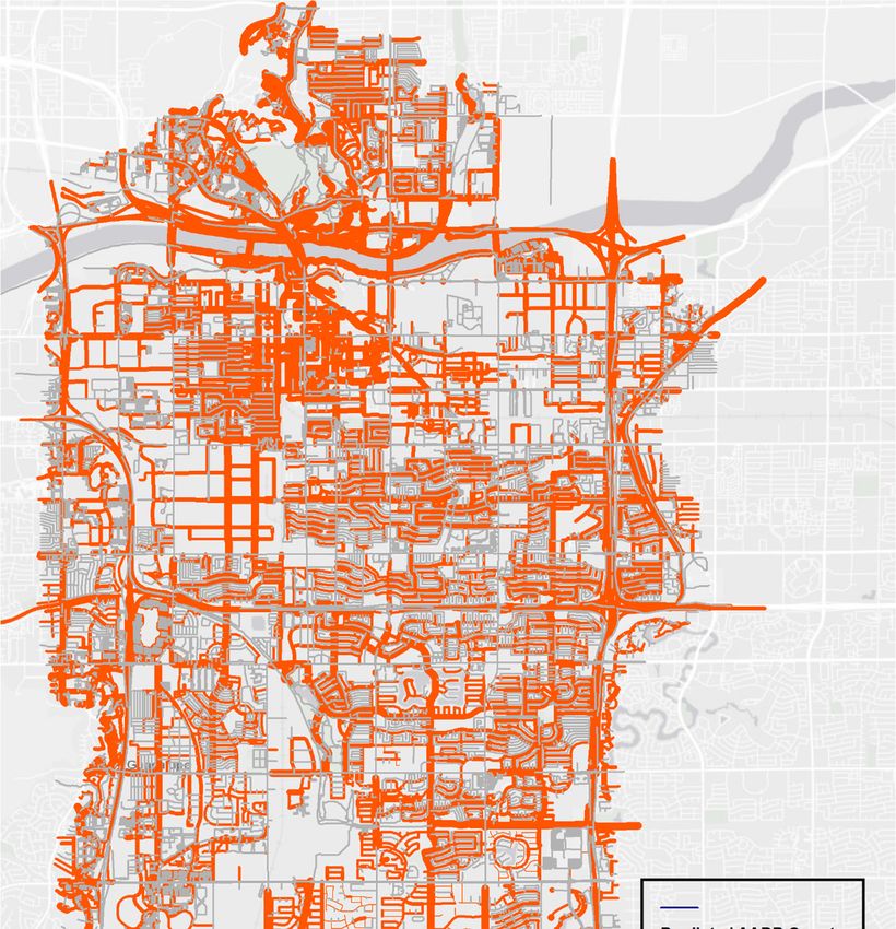
3.5. Mapping Predicted Ridership Volumes in Tempe
Based on our model, we predicted bias-corrected ridership volumes across the city of Tempe,
shown in Figure 7, classified using Jenks’ classification into five categories: Very low (0–25), low
(25–100), medium (100–750), high (750–2500), and very high (2500+). The thin lines indicate streets
with a low volume of bicyclists while the thicker lines indicate streets with a high volume of bicyclists.Urban Sci. 2019, 3, 62 14 of 20
Urban Sci. 2019, 3, x FOR PEER REVIEW 13 of 19
Figure 7. Predicted bicycle AADB counts for the entire street network of Tempe in 2016.
Figure 7. Predicted bicycle AADB counts for the entire street network of Tempe in 2016.
3.6.Prediction
3.6. PredictionAccuracy
Accuracyofofthe
theBias
BiasCorrection
CorrectionModel
ModelininTempe
Tempe
InFigure
In Figure8,8,the
theresult
resultofofthe
theprediction
predictionaccuracy
accuracyasasaafunction
functionof ofthe
thedifference
differenceininthe
thepredicted
predicted
AADBcounts
AADB countsfrom
fromthetheobserved
observedcounts
countsacross
across6060count
countlocations
locationsininTempe
Tempeisisgiven.
given.Urban Sci. 2019, 3, 62 15 of 20
Urban Sci. 2019, 3, x FOR PEER REVIEW 14 of 19
Figure8.8.Model
Figure ModelPrediction
PredictionAccuracy
Accuracyfor
forTempe
Tempeinin2016.
2016.
Overall,
Overall,for
for59%
59%of
ofthe
thesegments,
segments,we
wepredicted
predictedridership
ridershipvolumes within±50
volumeswithin ±50AADB,
AADB,86%
86%of
ofthe
the
segments
segmentswere withinaa±100
werewithin ±100AADB,
AADB,and
and95% within±200
95%within ±200 AADB.
AADB.
4.4.Discussion
Discussion
We
Wewere
wereable abletotocorrect
correctthe thebias
biasinincrowdsourced
crowdsourceddata datafrom
fromStrava
Stravausingusingaasetsetofofcovariates
covariates
describing the street location and from this we were able to generate
describing the street location and from this we were able to generate maps representative maps representative of all bicyclists
of all
at a street-level
bicyclists spatial resolution.
at a street-level The correlation
spatial resolution. between the
The correlation Strava the
between andStrava
officialand
counts alone
official can
counts
explain
alone can nearly
explain52%nearly
of the52%variation in overallinbicycle
of the variation overallridership, however,however,
bicycle ridership, we werewe limited
were by the
limited
availability of ground truth data, which could help improve the R 2 further. Our goal in combining
by the availability of ground truth data, which could help improve the R2 further. Our goal in
geographic
combining covariates
geographic with Strava counts
covariates was to account
with Strava counts was for additional
to accountfactors that influence
for additional factorsbicycle
that
ridership
influence and mayridership
bicycle not be captured
and may solelynot by be crowdsourced
captured solely sampling. These variables
by crowdsourced sampling.helped in
These
making necessary adjustments for the estimation of observed counts
variables helped in making necessary adjustments for the estimation of observed counts of all of all bicyclists, including those
not using the
bicyclists, Strava app,
including those thereby
not usingcorrecting bias in
the Strava crowdsourced
app, data from
thereby correcting biasStrava.
in crowdsourced data
The Poisson
from Strava. regression approach has frequently been used in bicycle crash analysis by [10,35] as
well as for exposure measurement of accidents by [50]. A probabilistic
The Poisson regression approach has frequently been used in bicycle crash analysis joint analysis approach
by [10] hasand
been used for correcting sampling bias in species distribution models by [51].
[35] as well as for exposure measurement of accidents by [50]. A probabilistic joint analysis approach Using the mixed-model
approach, this paper
has been used proposes asampling
for correcting new technique
bias ininspecies
the bias correction of
distribution crowdsourced
models data for
by [51]. Using thephysical
mixed-
activity mapping from bicycle ridership.
model approach, this paper proposes a new technique in the bias correction of crowdsourced data
The results
for physical of our
activity study indicate
mapping from bicycle that bias correction of crowdsourced data may prove to be a
ridership.
usefulThemethod for the estimation of bicycle ridership
results of our study indicate that bias correction in North ofAmerican
crowdsourced cities. data
Our may
results for the
prove to city
be a
of Tempe (Figure 7) indicate that for 80.3% of road segments, where ground
useful method for the estimation of bicycle ridership in North American cities. Our results for the truth data were available,
estimated bicycle
city of Tempe counts7)
(Figure were correct
indicate to within
that for 80.3% 25%of ofroad
the observed
segments, counts
where (± ground
50 riders). Ourdata
truth findings
were
are in alignment with recent research by [15,20], who found strong relationships
available, estimated bicycle counts were correct to within 25% of the observed counts (± 50 riders). between Strava and
all
Ourbicycling
findingsridership in North with
are in alignment American
recentcities.
research by [20] and [15], who found strong relationships
As expected, the proximity
between Strava and all bicycling ridership of a street segment
in North to a residential
American cities.neighborhood had a significant
influence on the overall bicycle ridership. Most segments
As expected, the proximity of a street segment to a residential that are close to a residential
neighborhood hadarea in Tempe
a significant
have betteron
influence road
theinfrastructure,
overall bicycleincluding
ridership.paved Most sidewalks
segments that and are
dedicated
close tobike lanes. This
a residential encourages
area in Tempe
have better road infrastructure, including paved sidewalks and dedicated bike lanes. This encourages
inexperienced bicyclists to ride safely and also adds comfort to the overall bicycling experience inUrban Sci. 2019, 3, 62 16 of 20
inexperienced bicyclists to ride safely and also adds comfort to the overall bicycling experience in
general for riders of all ages and abilities. Hence, transportation planners should pay more attention
to the use of wider streets with dedicated bike lanes in residential areas to help increase active
transportation among riders irrespective of their age and ability. Similarly, a closer proximity to green
space also had a positive influence on ridership. One reason for the relationship between bicycling and
green space may be that green corridors, which connect the bicycle network within a city, facilitate
increased overall bicycle ridership.
The positive coefficients for Strava counts and the white population percentage are in alignment
with the fact that ethnicity influences ridership and that in urban areas, generally, a higher proportion
of white residents ride bicycles than non-white residents. Previous studies by [32,52] have shown that
positive relationships exist between ethnicity (white, non-white) and physical activity. Our model
results also show that ethnicity is an important factor to use when correcting bias Strava sampled
bicycle ridership volumes.
Median household income was also significant in influencing overall bicycling ridership. It has
been found in previous research [53] that people from lower economic backgrounds are less likely to
adopt an active lifestyle and our results also indicate a similar trend. Bicycling should be made more
cost-effective for daily use by commuters in order to promote active transportation.
High speed limits are often correlated with roads having greater concentrations of larger-sized
vehicles and more traffic, both of which are major deterrents to bicycling in general [32,39] and often
result in crashes [54]. These results suggest policy directions for the safety of bicyclists by means of the
reduction of speed limits on busy traffic corridors, and the provision of dedicated bike lanes or green
zones on major streets connecting areas of interest (schools, business centers, parks, shopping complex,
etc.) to attract riders of all ages and abilities.
The model framework proposed in this study can be used for correcting bias in Strava riders
from other cities or bicyclist counts comparable in space and time obtained from other bicycling
apps. However, our study has a few limitations. The official counts from the MAG were collected
at 44 locations scattered across the whole of Maricopa County. As the segments containing available
ground truth data were mostly within the city limits, data from open spaces on the outskirts of cities
were sparse. The choice of geographic covariates was specific to the study area and might vary for
different geographic settings, depending upon their relevance. The model could have been improved
in terms of the prediction accuracy if more ground truth data were available across diverse locations to
train the model. Street conditions with a low prediction accuracy can be targeted for future sampling
and organized data collection efforts can be proposed for better quality data, which could help in the
improvement of the model. With the availability of sufficient data, further studies could examine the
spatial heterogeneity of bias-corrected ridership across varying geographies using localized regression
on more realistic conditions across larger spatial scales.
5. Conclusions
Big crowdsourced data from fitness apps, like Strava, on bicycling volumes can be used to make
informed decisions on factors that influence ridership in urban areas on a much finer spatial scale.
We introduced a new method for correcting bias in crowdsourced data with the help of a three-step
mixed-model approach by quantifying crowdsourced data and official counts in a specific geographic
region, using LASSO to choose the most significant geographic variables that could correct bias, and
finally, fitting the covariates along with the crowdsourced data by means of Poisson regression to
predict and map overall ridership in the region. The method developed in this study is broadly
applicable for correcting bias in crowdsourced bicycling data when official counts and geographical
data are available at comparable spatial and temporal resolution. Based on the results of this paper,
in the future, it is suggested that local transportation authorities should work closely with researchers
to improve the coverage of official count data, helping them to identify locations to place counters so
that a denser spatial coverage as well as more ground truth data are obtained to improve the model’sUrban Sci. 2019, 3, 62 17 of 20
performance. The proposed bias correction model, with detailed data that is continuous through
space and collected repeatedly in time, can help transportation planners in making informed decisions
related to bicycle infrastructure planning to promote healthier lifestyles among urban residents of
all ages and abilities. Detailed maps of bicycling ridership are critical to professionals in making
decisions regarding infrastructure investment and policy changes that support active transportation.
The framework developed in this paper can be used as a generalized risk assessment and exposure
modeling tool to benefit accident prevention among bicyclists, with sufficient availability of accident
data from crowdsourced platforms, like Bikemaps.org [19], and provide an estimate of bias-corrected
bicyclist volumes for infrastructure planning to enhance comfort among bicyclists and promote active
modes of transportation for healthier lifestyles among wider demographics.
Supplementary Materials: The following are available online at http://www.mdpi.com/2413-8851/3/2/62/s1.
Author Contributions: A.R. developed the algorithms and code, analyzed and interpreted the Strava and MAG
data regarding the bicyclist counts, and performed the modeling and analyses. T.A.N. organized the data collection
effort, identified the research gap, contributed to the verification of the results, and was a major contributor in
writing the manuscript. A.S.F. was a major contributor in developing robust analytical methods, interpreting
the results, and editing and writing the manuscript. M.W. helped in the overall organization of the manuscript
and contributed in reviewing the results and communicating the context. All authors read and approved the
final manuscript.
Funding: This research was funded by Arizona State University.
Acknowledgments: The authors would like to acknowledge Jason Stephens and Vladimir Livshits from the MAG
for providing ground truth data from Maricopa County. They are also grateful to the Strava team led by Brian
Riordan for kindly sharing the Strava ridership data for Maricopa County. Additionally, we thank the Tempe
Bicycle Association Group and Cliff Anderson specifically for providing access to the Tempe bicycle counts data
and ongoing support throughout the project.
Conflicts of Interest: The authors declare no conflict of interest. The funders had no role in the design of the
study; in the collection, analyses, or interpretation of data; in the writing of the manuscript, or in the decision to
publish the results.
Abbreviations
MAG Maricopa Association of Governments
TBAG Tempe Bicycle Action Group
LASSO Least absolute shrinkage and selection operator
PANDAS Python data analysis library
AADB Average annual daily bicyclists
VIF Variance Inflation Factor
References
1. Sallis, J.F.; Floyd, M.F.; Rodríguez, D.A.; Saelens, B.E. Role of built environments in physical activity, obesity,
and cardiovascular disease. Circulation 2012, 125, 729–737. [CrossRef]
2. Colberg, S.R.; Sigal, R.J.; Fernhall, B.; Regensteiner, J.G.; Blissmer, B.J.; Rubin, R.R.; Chasan-Taber, L.;
Albright, A.L.; Braun, B.; American College of Sports Medicine; et al. Exercise and type 2 diabetes:
The American College of Sports Medicine and the American Diabetes Association: joint position statement
executive summary. Diabetes Care 2010, 33, 2692–2696. [CrossRef] [PubMed]
3. Kushi, L.H.; Doyle, C.; McCullough, M.; Rock, C.L.; Demark-Wahnefried, W.; Bandera, E.V.; Gapstur, S.;
Patel, A.V.; Andrews, K.; Gansler, T.; et al. American Cancer Society guidelines on nutrition and physical
activity for cancer prevention: Reducing the risk of cancer with healthy food choices and physical activity.
CA Cancer J. Clin. 2012, 62, 30–67. [CrossRef] [PubMed]
4. World Health Organization (WHO). Global Recommendations on Physical Activity for Health: World Health
Organization; World Health Organization (WHO): Geneve, Switzerland, 2010.
5. Mansfield, T.J.; Gibson, J.M. Estimating Active Transportation Behaviors to Support Health Impact Assessment
in the United States. Front. Public Health 2016, 4, 591. [CrossRef] [PubMed]Urban Sci. 2019, 3, 62 18 of 20
6. Lyons, W.; Peckett, H.; Morse, L.; Khurana, M.; Nash, L. Metropolitan Area Transportation Planning for Healthy
Communities; No. DOT-VNTSC-FHWA-13-01; John A. Volpe National Transportation Systems Center: Boston,
MA, USA, 2012.
7. Larsen, J.; Patterson, Z.; El-Geneidy, A. Build It. But Where? The Use of Geographic Information Systems in
Identifying Locations for New Cycling Infrastructure. Int. J. Sustain. Transp. 2013, 7, 299–317. [CrossRef]
8. Lovelace, R.; Goodman, A.; Aldred, R.; Berkoff, N.; Abbas, A.; Woodcock, J. The Propensity to Cycle Tool:
An open source online system for sustainable transport planning. J. Transport Land Use 2017, 10, 505–528.
[CrossRef]
9. Ryus, P.; Ferguson, E.; Laustsen, K.M.; Schneider, R.J.; Proulx, F.R.; Hull, T.; Miranda-Moreno, L. National
Academies of Sciences, Engineering, and Medicine; Transportation Research Board; National Cooperative
Highway Research Program. In Methods and Technologies for Pedestrian and Bicycle Volume Data Collection;
The National Academies Press: Washington, DC, USA, 2014.
10. Griswold, J.B.; Medury, A.; Schneider, R.J.; Information, R. Pilot Models for Estimating Bicycle Intersection
Volumes. Transp. Res. Rec. J. Transp. Res. Board 2011, 2247, 1–7. [CrossRef]
11. Nordback, K.; Marshall, W.E.; Janson, B.N.; Stolz, E. Estimating annual average daily bicyclists: Error and
accuracy. Transp. Res. Rec. J. Transp. Res. Board 2013, 2339, 90–97. [CrossRef]
12. Griffin, G.; Nordback, K.; Götschi, T.; Stolz, E.; Kothuri, S. Monitoring Bicyclist and Pedestrian Travel and
Behavior: Current Research and Practice. Transportation Research Circular E-C18. 2014. Available online:
http://www.trb.org/Publications/Blurbs/170452.aspx (accessed on 31 May 2018).
13. El Esawey, M.; Mosa, A.I.; Nasr, K. Estimation of daily bicycle traffic volumes using sparse data.
Comput. Environ. Urban Syst. 2015, 54, 195–203. [CrossRef]
14. Shen, L.; Stopher, P.R. Review of GPS Travel Survey and GPS Data-Processing Methods. Transp. Rev. 2014,
34, 316–334. [CrossRef]
15. Griffin, G.P.; Jiao, J. Where does bicycling for health happen? Analysing volunteered geographic information
through place and plexus. J. Transp. Health 2015, 2, 238–247. [CrossRef]
16. Heesch, K.C.; Langdon, M. The usefulness of GPS bicycle tracking data for evaluating the impact of
infrastructure change on cycling behaviour. Health Promot. J. Aust. 2016, 27, 222–229. [CrossRef]
17. Bíl, M.; Andrášik, R.; Kubeček, J. How comfortable are your cycling tracks? A new method for objective
bicycle vibration measurement. Transp. Res. Part C: Emerg. Technol. 2015, 56, 415–425. [CrossRef]
18. Winters, M.; Brauer, M.; Setton, E.M.; Teschke, K. Built Environment Influences on Healthy Transportation
Choices: Bicycling versus Driving. J. Urban Health 2010, 87, 969–993. [CrossRef]
19. Nelson, T.A.; DenOuden, T.; Jestico, B.; Laberee, K.; Winters, M. BikeMaps.org: A Global Tool for Collision
and Near Miss Mapping. Front. Public Health 2015, 3, 53. [CrossRef]
20. Jestico, B.; Nelson, T.; Winters, M. Mapping ridership using crowdsourced cycling data. J. Geogr. 2016, 52,
90–97. [CrossRef]
21. Strava.com. Strava Metro. Strava, April 2018. Available online: https://metro.strava.com/ (accessed on
28 April 2018).
22. Lieske, S.N.; Leao, S.Z.; Conrow, L.; Pettit, C.J. Validating Mobile Phone Generated Bicycle Route Data in
Support of Active Transportation. In Proceedings of the SOAC 2017—State of Australian Cities (SOAC)
National Conference, Adelaide, South Australia, 28–30 November 2017.
23. Feick, R.; Roche, S. Understanding the Value of VGI. In Crowdsourcing Geographic Knowledge; Sui, D., Elwood, S.,
Goodchild, M., Eds.; Springer: Dordrecht, The Netherlands, 2013; pp. 15–29.
24. Solymosi, R.; Bowers, K.J.; Fujiyama, T. Crowdsourcing Subjective Perceptions of Neighbourhood Disorder:
Interpreting Bias in Open Data. Br. J. Criminol. 2017, 58, 944–967. [CrossRef]
25. Ton, D.; Duives, D.; Cats, O.; Hoogendoorn, S. Evaluating a data-driven approach for choice set identification
using GPS bicycle route choice data from Amsterdam. Travel Behav. Soc. 2018, 13, 105–117. [CrossRef]
26. Sun, Y.; Mobasheri, A. Utilizing Crowdsourced Data for Studies of Cycling and Air Pollution Exposure:
A Case Study Using Strava Data. Int. J. Environ. Res. Public Health 2017, 14, 274. [CrossRef]
27. Maricopa Association of Governments. MAG Bike Counts Initiative 2016. Available online:
azmag.gov/Portals/0/Documents/BaP_2014-09-16_Item-07_MAG-Bicycles-Count-Project-Presentation.
pdf?ver=2017-04-06-110803 (accessed on 6 April 2017).
28. US Census Bureau Geography. Cartographic Boundary Shapefiles—Counties. 1 September 2012. Available
online: https://www.census.gov/geo/maps-data/data/cbf/cbf_counties.html (accessed on 6 April 2018).Urban Sci. 2019, 3, 62 19 of 20
29. City of Tempe. Tempe Transportation Master Plan. 2015. Available online: http://www.tempe.gov/home/
showdocument?id=30317 (accessed on 20 April 2018).
30. Saelens, B.E.; Sallis, J.F.; Frank, L.D. Environmental correlates of walking and cycling: Findings from the
transportation, urban design, and planning literatures. Ann. Behav. Med. 2003, 25, 80–91. [CrossRef]
31. Moudon, A.V.; Lee, C.; Cheadle, A.D.; Collier, C.W.; Johnson, D.; Schmid, T.L.; Weather, R.D. Cycling and the
built environment, a US perspective. Transp. Res. Part D Transp. Environ. 2005, 10, 245–261. [CrossRef]
32. Winters, M.; Teschke, K.; Grant, M.; Setton, E.M.; Brauer, M. How far out of the way will we travel?: Built
environment influences on route selection for bicycle and car travel. Transp. Res. Rec. J. Transp. Res. Board
2010, 2190, 1–10. [CrossRef]
33. Sallis, J.F.; Conway, T.L.; Dillon, L.I.; Frank, L.D.; Adams, M.A.; Cain, K.L.; Saelens, B.E. Environmental and
Demographic Correlates of Bicycling. Prev. Med. 2013, 57, 456–460. [CrossRef]
34. Nehme, E.K.; Pérez, A.; Ranjit, N.; Amick, B.C., III; Kohl, H.W., III. Sociodemographic factors, population
density, and bicycling for transportation in the United States. J. Phys. Act. Health 2016, 13, 36–43. [CrossRef]
35. Hankey, S.; Lindsey, G.; Wang, X.; Borah, J.; Hoff, K.; Utecht, B.; Xu, Z. Estimating use of non-motorized
infrastructure: Models of bicycle and pedestrian traffic in Minneapolis, MN. Landsc. Urban Plan. 2012, 107,
307–316. [CrossRef]
36. Plaut, P.O. Non-motorized commuting in the US. Transp. Res. Part D Transp. Environ. 2005, 10, 347–356.
[CrossRef]
37. Sallis, J.F.; Saelens, B.E.; Frank, L.D.; Conway, T.L.; Slymen, D.J.; Cain, K.L.; Chapman, J.E.; Kerr, J.
Neighborhood Built Environment and Income: Examining Multiple Health Outcomes. Soc. Sci. Med. 2009,
68, 1285–1293. [CrossRef]
38. Strauss, J.; Miranda-Moreno, L.F. Spatial modeling of bicycle activity at signalized intersections. J. Transp.
Land Use 2013, 6, 47. [CrossRef]
39. Piatkowski, D.P.; Marshall, W.E. Not all prospective bicyclists are created equal: The role of attitudes,
socio-demographics, and the built environment in bicycle commuting. Travel Behav. Soc. 2015, 2, 166–173.
[CrossRef]
40. Kluyver, T.; Ragan-Kelley, B.; Pérez, F.; Granger, B.E.; Bussonnier, M.; Frederic, J.; Kelley, K.; Hamrick, J.B.;
Grout, J.; Corlay, S.; et al. Jupyter Notebooks—A publishing format for reproducible computational
workflows. In Positioning and Power in Academic Publishing: Players, Agents and Agendas; IOS Press:
Amsterdam, The Netherlands, 2016; pp. 87–90.
41. Python Software Foundation. Python Language Reference, Version 3.5. Available online: http://www.python.
org (accessed on 31 May 2019).
42. R Core Team. R: A Language and Environment for Statistical Computing; R Foundation for Statistical Computing:
Vienna, Austria, 2013. Available online: http://www.R-project.org (accessed on 31 May 2019).
43. McKinney, W. Python for Data Analysis: Data Wrangling with Pandas, NumPy, and Ipython; O’Reilly Media Inc.:
Sebastopol, CA, USA, 2012.
44. Crawley, M.J. Statistics: An Introduction Using R; Wiley: Hoboken, NJ, USA, 2005; ISBN 0 470.02298.
45. Jordahl, K. GeoPandas: Python Tools for Geographic Data. Geopandas, 2014. Available online: https:
//github.com/geopandas/geopandas (accessed on 31 May 2019).
46. Tibshirani, R. Regression Shrinkage and Selection via the Lasso. J. R. Stat. Soc. Ser. B (Methodol.) 1996, 58,
267–288. [CrossRef]
47. Meinshausen, N.; Bühlmann, P. Stability selection. J. R. Stat. Soc. Ser. B (Methodol.) 2010, 72, 417–473.
[CrossRef]
48. Dobson, A.J.; Barnett, A.G. An Introduction to Generalized Linear Models; CRC Press: Boca Raton, FL, USA,
2008; ISBN 9781138741515.
49. Kohavi, R. A study of cross-validation and bootstrap for accuracy estimation and model selection.
In Proceedings of the 14th International Joint Conference on Artificial Intelligence (IJCAI’95), Montreal, QC,
Canada, 20–25 August 1995; Morgan Kaufmann Publishers Inc.: San Francisco, CA, USA, 1995; Volume 2.
50. Hamann, C.; Peek-Asa, C. On-road bicycle facilities and bicycle crashes in Iowa, 2007–2010. Accid. Anal.
Prev. 2013, 56, 103–109. [CrossRef]
51. Fithian, W.; Elith, J.; Hastie, T.; Keith, D.A. Bias correction in species distribution models: pooling survey and
collection data for multiple species. Methods Ecol. Evol. 2015, 6, 424–438. [CrossRef]You can also read