Operational Wave Forecast Selection in the Atlantic Ocean Using Random Forests
←
→
Page content transcription
If your browser does not render page correctly, please read the page content below
Journal of
               Marine Science
               and Engineering

Article
Operational Wave Forecast Selection in the Atlantic Ocean
Using Random Forests
Ricardo M. Campos, Mariana O. Costa, Fabio Almeida and C. Guedes Soares *

                                           Centre for Marine Technology and Ocean Engineering (CENTEC), Instituto Superior Técnico, Universidade de
                                           Lisboa, Av. Rovisco Pais, 1049-001 Lisboa, Portugal; ricardo.campos@centec.tecnico.ulisboa.pt (R.M.C.);
                                           mariana.costa@centec.tecnico.ulisboa.pt (M.O.C.); fabio.almeida@centec.tecnico.ulisboa.pt (F.A.)
                                           * Correspondence: c.guedes.soares@centec.tecnico.ulisboa.pt

                                           Abstract: The existence of multiple wave forecasts leads to the question of which one should be
                                           used in practical ocean engineering applications. Ensemble forecasts have emerged as an important
                                           complement to deterministic forecasts, with better performances at mid-to-long ranges; however,
                                           they add another option to the variety of wave predictions that are available nowadays. This study
                                           developed random forest (RF) postprocessing models to identify the best wave forecast between
                                           two National Centers for Environmental Protection (NCEP) products (deterministic and ensemble).
                                           The supervised learning classifier was trained using National Data Buoy Center (NDBC) buoy data
                                           and the RF model accuracies were analyzed as a function of the forecast time. A careful feature
                                           selection was performed by evaluating the impact of the wind and wave variables (inputs) on the
                                           RF accuracy. The results showed that the RF models were able to select the best forecast only in the
                                           very short range using input information regarding the significant wave height, wave direction and
                                 period, and ensemble spread. At forecast day 5 and beyond, the RF models could not determine

                                           the best wave forecast with high accuracy; the feature space presented no clear pattern to allow for
Citation: Campos, R.M.; Costa, M.O.;       successful classification. The challenges and limitations of such RF predictions for longer forecast
Almeida, F.; Guedes Soares, C.             ranges are discussed in order to support future studies in this area.
Operational Wave Forecast Selection
in the Atlantic Ocean Using Random
                                           Keywords: wave forecasts; random forests; decision trees; numerical wave modeling; ensemble
Forests. J. Mar. Sci. Eng. 2021, 9, 298.
                                           forecasting; extreme events; data mining
https://doi.org/10.3390/
jmse9030298

Academic Editor: Decheng Wan
                                           1. Introduction
Received: 27 January 2021                        Operational wave forecasts provide key information for several ocean engineering
Accepted: 20 February 2021                 activities, from ship routing to a range of maritime operations [1–3]. The significant wave
Published: 8 March 2021                    height (Hs) is one of the most important parameters that are associated with the description
                                           of the sea state intensity and acts as an input to specific models involving safety, logistics,
Publisher’s Note: MDPI stays neutral       and stability [4]. The main objective in weather routing systems is to plan maritime
with regard to jurisdictional claims in    operations, including normal ship voyages and making adjustments to avoid storms [5],
published maps and institutional affil-    which are critical situations regarding the safety of operation. Therefore, in many situations,
iations.                                   wave forecasts need to be specially designed to improve their performance in predicting
                                           storms [6,7], although, in some situations, other approaches are used to identify and track
                                           cyclones [8,9].
                                                 A great challenge, however, is related to wave forecasts, which is a complex task that
Copyright: © 2021 by the authors.          is strongly dependent on the quality of the surface wind data [10]. Large forecast errors
Licensee MDPI, Basel, Switzerland.         are associated with longer forecast lead times and extreme conditions, as discussed in [11],
This article is an open access article     due to the chaotic behavior of the atmosphere, as described in [12,13]. The implementation
distributed under the terms and            of wave ensemble forecasting systems in the 2000s represented a major improvement to
conditions of the Creative Commons         forecasting ability, especially beyond a 5-day forecast horizon [14,15]. The ensemble mean
Attribution (CC BY) license (https://      (EM) of several perturbed independent simulations (members) was shown to have higher
creativecommons.org/licenses/by/           correlation coefficients and lower scatter errors when compared to traditional deterministic
4.0/).

J. Mar. Sci. Eng. 2021, 9, 298. https://doi.org/10.3390/jmse9030298                                           https://www.mdpi.com/journal/jmse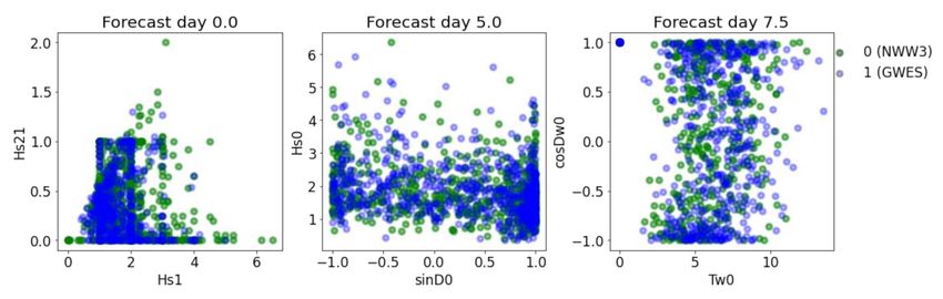
J. Mar. Sci. Eng. 2021, 9, 298                                                                                              2 of 17

                                 forecasts. Therefore, despite the coarser spatial resolution, ensemble wave forecasts have
                                 become an important source of wave prediction at extended forecast ranges.
                                       The analyses of [16,17], based on data from the National Centers for Environmental
                                 Prediction/National Oceanic and Atmospheric Administration (NCEP/NOAA), have shown
                                 that, on average, deterministic wave forecasts present the best results for the first four or five
                                 days, while ensemble forecasts have the best performances beyond one week. Nevertheless,
                                 these are overall assessments and the forecast model with the lowest Hs errors might change
                                 depending on the metocean conditions and location. Therefore, the selection of the most
                                 accurate wave forecast product is not a straightforward task and becomes even more
                                 complex when multiple forecasts are included, such as those evaluated by [18]. In this
                                 context, the present study aimed to compare two operational wave forecasts from the
                                 NCEP and to develop a machine learning model using random forests (RFs) to identify
                                 the prediction with the lowest Hs error. This approach allows for postprocessing different
                                 wave forecasts and to provide a single estimation of Hs that can be directly used in other
                                 applications of interest in maritime engineering. Attention was dedicated to identifying the
                                 best combination of features, followed by the optimal depth of the trees, and the number
                                 of trees in the forest.
                                       Soft computing techniques have been widely used to predict wave parameters [19–23].
                                 Modern neural wavelet techniques were implemented in [24,25], hybrid empirical orthogo-
                                 nal function (EOF)-wavelet modeling was further developed in [26], and support vector
                                 machine models were discussed in [27]. As a representative example of machine learning
                                 algorithms, the decision tree models adopt recursive segmentation technology to continu-
                                 ously divide the data space into subsets to detect the potential structure, important patterns,
                                 and dependencies of data. As the decision between two wave predictions is essentially
                                 an uncertain and partially random process, it is not easy to accurately achieve the proper
                                 selection using deterministic equations or drawing conclusions from bulk error metrics
                                 and general assessments. Therefore, it is ideally suited to decision trees and random forests
                                 since they are primarily aimed at the recognition of a random pattern in a given set of input
                                 values. Examples of applications in wave modeling are given in [28,29].
                                       This paper is organized as follows. Section 2 describes the datasets, including the
                                 forecast data from the NCEP and buoy data from the National Data Buoy Center (NDBC),
                                 as well as the data structure and dimensions. Section 3 contains the feature selection,
                                 where 35 environmental variables are analyzed, followed by the random forest model
                                 description and the optimization of hyperparameters. Section 4 presents the results and
                                 discusses the RF accuracies at different forecast ranges. Section 5 contains the summary of
                                 the final conclusions.

                                 2. Data Description
                                      The forecast products for the study consisted of publicly available wind and wave
                                 operational global forecasts from the NCEP. Since waves are generated by surface winds,
                                 the atmospheric information was also included to improve the machine learning perfor-
                                 mance. The quality of wave simulations associated with the input winds is discussed
                                 by [30,31]. For the model assessments and random forest training, five metocean buoys
                                 were selected in the North Atlantic Ocean.

                                 2.1. Operational Wave Forecasts
                                      The operational forecast data from the NCEP included both deterministic and ensem-
                                 ble products of winds and waves. In summary, an ensemble forecast performs several
                                 numerical model integrations simultaneously with perturbations applied to the initial
                                 conditions or the model parameters. This has two main advantages: (i) the average (arith-
                                 metic EM) of the multiple simulations (ensemble members) can smooth out uncertain
                                 components, which leads to better results than a single deterministic forecast, and (ii) the
                                 spread of the ensemble members provides an estimation of the uncertainty of the prediction.
                                 The disadvantages of ensemble forecasts are associated with the high computational cost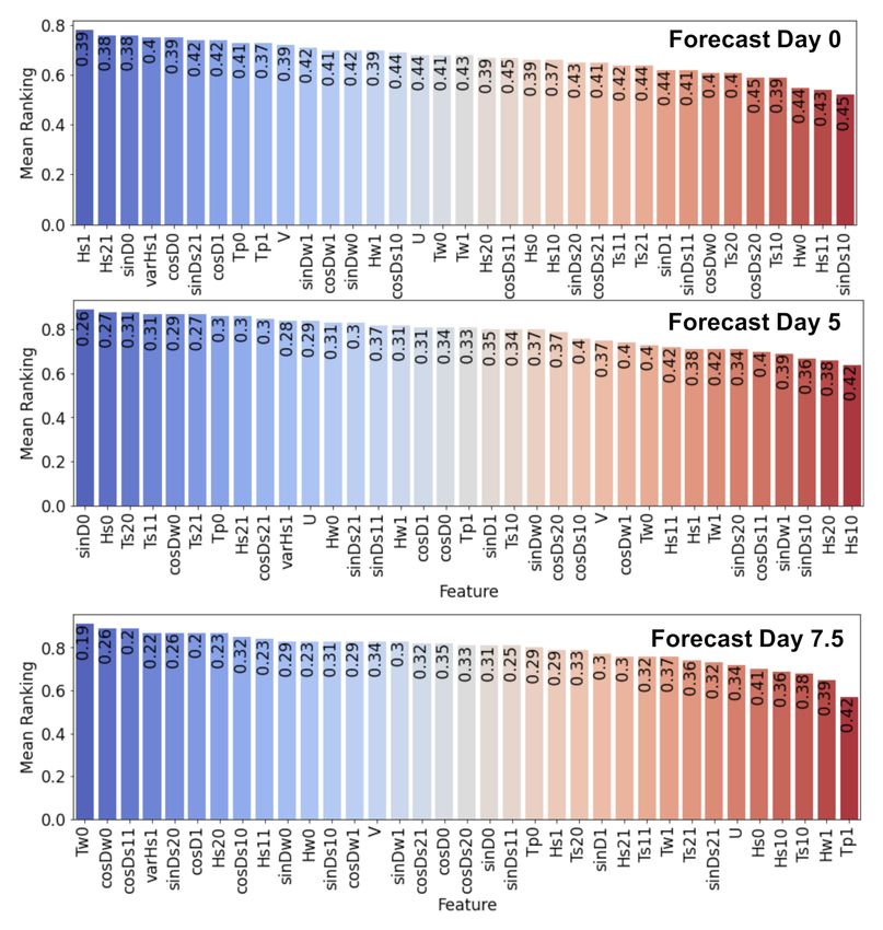
J. Mar. Sci. Eng. 2021, 9, 298 3 of 17
of running multiple simulations, which leads operational centers to implement coarser res-
olutions, which can compromise the representation of certain scales and locations; in these
cases, deterministic forecasts overperform the ensemble forecasts.
The deterministic NCEP wind forecast selected for this study came from the Global
Forecast System (GFS), while the ensemble came from the Global Ensemble Forecast
System [32]. In June 2019, the NCEP atmospheric forecast had a major upgrade, moving to
the Finite-Volume Cubed-Sphere dynamical core (FV3) developed in the NOAA Research’s
Geophysical Fluid Dynamics Laboratory, which is described at https://www.weather.gov/
news/fv3 (accessed on 1 November 2020) and https://www.gfdl.noaa.gov/fv3/ (accessed
on 1 November 2020).
The wind fields are inputs to the third-generation wave model WAVEWATCH III [33],
with a wave generation source term formulated by [34]. The same numerical wave model
is used to produce the deterministic and the ensemble wave forecasts, although differences
exist in terms of the configuration and spatial resolutions. In September 2020, new upgrades
in the NCEP/NOAA forecasts were put into operation.
In machine learning, it is important to pick forecast data (inputs) from the same
system version, i.e., the random forest should not be trained with the model physics,
calibrations, and resolutions changing in the middle of the dataset. Otherwise, the relations
between variables would drastically change within the same dataset and such heterogeneity
could compromise the optimization and future predictions. The required consistency is
guaranteed in the period between 25-09-2019 and 01-07-2020, which was selected for the
present study. The forecast products and resolutions utilized can be summarized as follows
(spatial resolutions of the global grids are indicated within the brackets):
(1) Deterministic Global Forecast System (GFS) from NCEP/NOAA (0.117◦ × 0.117◦ );
(2) Global Ensemble Forecast System (GEFS) from NCEP/NOAA (0.5◦ × 0.5◦ ), with
20 members;
(3) Deterministic Wave Forecast System based on WAVEWATCH III model (NWW3)
from NCEP/NOAA (0.5◦ × 0.5◦ );
(4) Global Ocean Wave Ensemble Forecast System (GWES) from NCEP/NOAA (0.5◦ × 0.5◦ ),
with 20 members.
From the wind and wave fields, single points were extracted by taking the buoy’s
positions and using a bi-linear weighted (by distance) average of the surrounding grid
points, following [11]. The multiple forecast variables were later analyzed to evaluate the
influence of each variable in distinguishing the NWW3 and GWES errors of Hs, and to
exclude the ones that did not contribute; this process is called feature selection, as discussed
in the next section.
2.2. Buoy Data
The buoy data were obtained from the NDBC/NOAA by choosing the metocean
buoys with similar characteristics, which provided wave and atmospheric parameters.
Shallow water buoys close to the coast were excluded and the data were carefully in-
spected to select buoys with the largest amount of quality data in the North Atlantic Ocean.
Five NDBC buoys were chosen, namely, 41047, 41048, 41049, 44008, and 44009, shown in
Figure 1. They are positioned in the western portion of the North Atlantic Ocean, at lati-
tudes from 26◦ to 41◦ N, and are under the influence of tropical and extra-tropical cyclones.
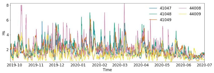
The Hs of the five NDBC buoys can be examined in Figure 2. Due to the location of
the buoys, i.e., in the same ocean basin, they tend to respond to the same storms, though
with severities varying depending on the storm tracks. Buoys 44009 and 44008 are more
influenced by extra-tropical cyclones, whereas 41047 and 41049 are more influenced by
tropical storms. Figure 2 shows several events reaching an Hs of 4 m and a few extreme
events at 7 to 8 m. The largest waves were measured by the NDBC buoy 44008 from
October to March.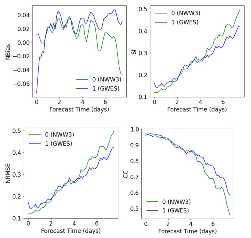
J. Mar. Sci. Eng. 2021, 9, 298                                                                                                4 of 17

                                     Figure 1. National Data Buoy Center (NDBC) buoys in the North Atlantic Ocean that were selected
                                     for the study.

                        Figure 2. Time series of the significant wave height Hs (meters) of the NDBC buoys selected.

                                     2.3. Data Arrays and Assessments
                                           The dataset pairs, including GFS/Buoy, NWW3/Buoy, and GWES/Buoy, resulted in
                                     3-hourly time series, which in fact had two time dimensions: (i) the forecast time selected
                                     varies from 0 (nowcast) to 648,000 s (7.5 days) with a step of 10,800 s (3 h) and (ii) the
                                     forecast cycle (each new simulation in the data archive) was selected once a day at 00Z.
                                     Therefore, considering, for example, the forecast cycle of 25-09-2019 00Z and forecast time
                                     of 7.5 days, the prediction values represent the time at 02-10-2019 12:00:00. Instead of using
                                     all ensemble members of GWES, which would represent another dimension in the data
                                     array, the arithmetic EM was calculated to directly compare with the deterministic model
                                     (NWW3). The ensemble spread of GWES was also computed and included in the input
                                     variables of the machine learning.
                                           As the prediction errors were the core of the study, a total of four metrics were intro-
                                     duced. The statistics were based on the study of [11] and following the discussion in [35].
                                     The error metrics used were the normalized bias (NBias), scatter index (SI), normalized
                                     RMSE (NRMSE), and the correlation coefficient (CC). Equations (1)–(4) describe the metrics
                                     selected, where x is the buoy data, y is the forecast, i is the index, n is the number of data
                                     points, and the overbar represents the mean of the variable. By using these normalized
                                     nondimensional metrics, the presented errors can be interpreted as ratios or percentage
                                     errors divided by 100.
                                                                                  ∑ n ( xi − yi )
                                                                        NBias = i=1 n                                            (1)
                                                                                     ∑ i =1 y i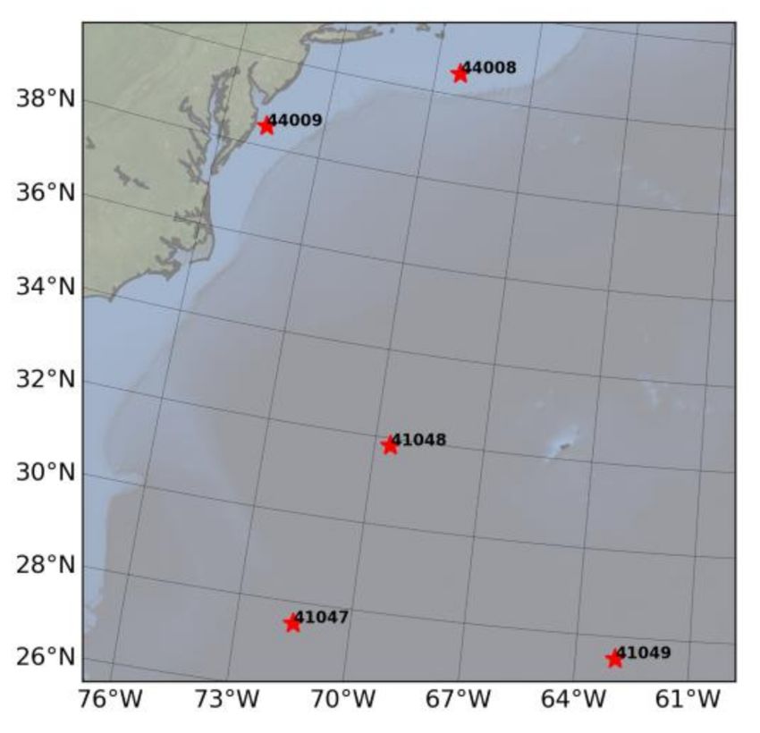
J. Mar. Sci. Eng. 2021, 9, 298                                                                                                 5 of 17

                                                                                                          2
                                                                       ∑in=1 [( xi − x ) − (yi − y)]
                                                                 SI =                                                             (2)
                                                                                   ∑in=1 yi 2
                                                                                 s
                                                                                                      2
                                                                                    ∑in=1 ( xi − yi )
                                                                     NRMSE =                                                      (3)
                                                                                        ∑in=1 yi 2
                                                                           ∑in=1 ( xi − x ) − (yi − y)
                                                              CC = q                                                              (4)
                                                                                         2                    2
                                                                          ∑in=1 ( xi − x ) ∑in=1 (yi − y)
                                      Error metrics were applied to assess the wave parameters at the five buoys. The eval-
                                 uation was performed as a function of the forecast time to compare the quality of the
                                 NWW3 and GWE (in terms of the EM) with increasing forecast leads. The results for NDBC
                                 buoy containing the most severe sea states, namely, ID 44008, are presented in Figure 3.
                                 The bias of the GWES on the nowcast was around −6%, indicating an overestimation of the
                                 arithmetic mean of the ensemble, which after the fourth day, became slightly positive with a
                                 small underestimation. In contrast, the bias of the NWW3 forecast was progressively lower
                                 with increasing forecast leads. The other three metrics indicated that the NWW3 in the first
                                 two forecast days gave the best results, whereas, after the fifth day, the ensemble (GWES)
                                 produced the best prediction of Hs. This result agrees with the previous assessments
                                 of [11,16,17]. It is out of the scope of the present study to provide a complete assessment of
                                 the NWW3 and GWES using NDBC data, as found in [11].

                                 Figure 3. Error metrics of Hs as a function of the forecast time for National Oceanic and Atmospheric
                                 Administration WAVEWATCH III (NWW3; in green) and Global Ocean Wave Ensemble Forecast
                                 System (GWES; in blue) at 40.50◦ N, 69.25◦ W. NBias: normalized bias, SI: scatter index, NRMSE:
                                 normalized root mean square error, CC: correlation coefficient.

                                 3. Methodology
                                 3.1. Description of the Variables
                                      The goal of the machine learning simulation was to obtain the best Hs prediction
                                 (between the two options) for each time step based on the wind and wave information
                                 from the NWW3, GWES, and GFS models. Therefore, the output variable (target) was
                                 the forecast model (class), “NWW3” or “GWES”, containing the lowest Hs error at each
                                 time step. The target was thus binary, with 0 corresponding to NWW3 and 1 to GWES.
                                 The inputs joined the wave and wind variables. The wave models predicted the following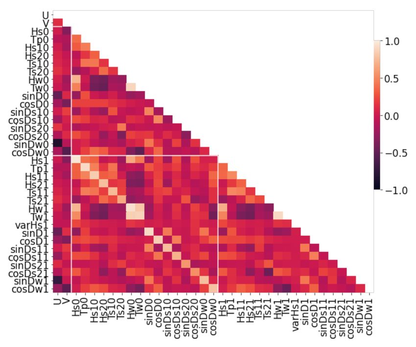
J. Mar. Sci. Eng. 2021, 9, 298                                                                                                     6 of 17

                                    variables of interest: wave direction, significant wave height, peak wave period, direction
                                    of the swell (partitions 1 and 2), significant wave height of the swell (partitions 1 and 2),
                                    period of the swell (partitions 1 and 2), significant wave height of the wind sea, period of
                                    the wind sea, and direction of the wind sea. The predicted variables of interest from the
                                    atmospheric model (GFS) were the zonal and meridional winds at 10 m. The directional
                                    variables were replaced by the sine and cosine and included in the feature space in order
                                    to include the direction cycle. This cycle had to be understood by the machine learning
                                    model since, for example, a direction of −180◦ comes after 179. The input variables were,
                                    initially, all the variables enumerated above, summarized in Table 1.
                                          Due to the strong dependence of Hs errors on the forecast lead time, as shown in
                                    Figure 3, it is important to analyze the machine learning performance as a function of
                                    the forecast range. Therefore, the datasets were divided into three groups in terms of the
                                    forecast times: day 0 (nowcast), day 5, and day 7.5. For each forecast time, data from the
                                    five locations (Figure 1) were appended into a single array to increase the dataset and
                                    sea-states available in an attempt to create stronger models.

      Table 1. Summary of the 35 input features, separated by forecast model. The names of the features adopted in the dataset
      are in the parenthesis.

        Forecast Model                                                           Variables
               GFS                                                        U-10m (U), V-10m (V)
                                   Significant wave height (Hs0), peak wave period (Tp0), partitions 1 and 2 of the Hs swell (Hs10 and
                                   Hs20), partitions 1 and 2 of the Tp swell (Ts10 and Ts20), wind sea Hs (Hw0), wind sea Tp (Tw0), sine
       NWW3 (model 0)
                                      and cosine of the wave direction D (sinD0 and cosD0), sine and cosine of the D swell partitions
                                   (sinDs10, cosDs10, sinDs20, and cosDs20), sine and cosine of the wind sea D (sinDw0 and cosDw0)
                                   Significant wave height (Hs1), peak wave period (Tp1), partitions 1 and 2 of the Hs swell (Hs11 and
                                     Hs21), partitions 1 and 2 of the Tp swell (Ts11 and Ts21), wind sea Hs (Hw1), wind sea Tp (Tw1),
        GWES (model 1)              variance of Hs of the ensemble members (varHs1), sine and cosine of the wave direction D (sinD1
                                   and cosD1), sine and cosine of the D swell partitions (sinDs11, cosDs11, sinDs21, and cosDs21), sine
                                                            and cosine of the wind sea D (sinDw1 and cosDw1)
                  GFS: Atmospheric Global Forecast System. NWW3: Deterministic Wave Forecast. GWES: Ensemble Wave Forecast.

                                          To analyze the class balance, a bar chart was created with the frequency of the classes’
                                    representations in the datasets for each forecast time, where class = 0 when NWW3 had
                                    the lowest Hs error and class = 1 when GWES had the lowest Hs error. Therefore, the two
                                    classes separated the two forecast options and its prediction indicated the choice between
                                    the wave forecasts, namely, NWW3 or GWES. Figure 4 presents the proportion of each class
                                    at the five spots, where the y-axis indicates the count of NWW3 or GWES representing the
                                    best choice. In total, 63.44% of the data in forecast day 0 was labeled 0 (NWW3); regarding
                                    forecast day 5, this percentage decreased to 51.57%, and on forecast day 7.5, this per-
                                    centage decreased further to 46.92%. The class evolution with forecast time agreed with
                                    Figure 3, where it was verified that NWW3 had the best overall predictions of Hs in the
                                    first few forecast days, and GWES produced the best predictions after the fifth day. How-
                                    ever, this feature was verified in terms of the class and decision between the two products.
                                    Moreover, Figure 4 adds important information to Figure 3, showing (and quantifying) that
                                    even for short-term forecasts, GWES might produce the best Hs predictions, and likewise,
                                    NWW3 can have the best results beyond 5-day forecasts, which is the opposite of what is
                                    suggested by Figure 3.
                                          The relation between variables was initially visualized through heatmaps of Pearson’s
                                    correlation coefficient, as shown in Figure 5. Note the last character in each abbreviation,
                                    which was used to differentiate between model 0 (NWW3) and model 1 (GWES), and are
                                    highlighted and separated in the figure with the white bold lines. As expected, pairs of
                                    highly correlated features were derived from the same environmental variables predicted
                                    using NWW3 and GWES. Even though there were high values of correlation between the
                                    variables, unnecessary feature removal can have a negative effect on model performance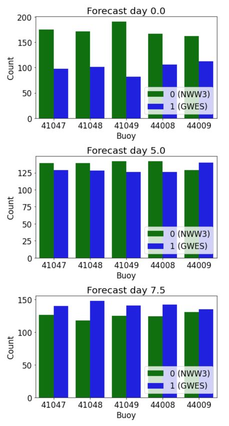
J. Mar. Sci. Eng. 2021, 9, 298                                                                                                 7 of 17

                                 and, thus, should be examined with caution. Hence, no feature was removed based on a
                                 threshold of the correlation score, thereby justifying a more appropriate feature selection
                                 methodology developed below.

                                 Figure 4. Proportion of the data in each class for the NDBC buoys for each forecast time. The x-axis
                                 shows the IDs of buoys, which can be visualized in Figure 1. The title of each plot indicates the
                                 forecast time associated.

                                 Figure 5. Correlation coefficients between all features for each dataset.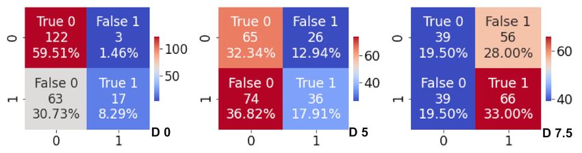
J. Mar. Sci. Eng. 2021, 9, 298                                                                                             8 of 17

                                 3.2. Feature Selection
                                       There are several ways to compute feature importance [36], with the most common
                                 method being the mean decrease in impurity (or Gini importance) [37], which is a mecha-
                                 nism that is biased [38]. A better alternative is the permutation importance, as described
                                 in [39], which is computationally more expensive but the results are more reliable. However,
                                 if several features are correlated and the estimator uses them all equally, the permutation
                                 importance can be low for all of these features; therefore, dropping one of the features may
                                 not affect the result, as the estimator still has access to the same information from other
                                 features. Consequently, if features are dropped based on the importance threshold, all such
                                 correlated features could be dropped at the same time, regardless of their usefulness.
                                       Recursive feature elimination (RFE) [40] and similar methods (as opposed to single-
                                 stage feature selection) can alleviate this problem. RFE is a wrapper algorithm that uses
                                 the learning process of a given machine learning model to identify an optimal set of
                                 variables among all possible alternatives. This procedure requires an update of the ranking
                                 criterion at each step of a backward strategy: the criterion is evaluated and the variable that
                                 minimizes this measure is eliminated. The ranking is then produced using the permutation
                                 importance measure, as it gives more precise results than the default feature importance
                                 measure of random forests [41]. The use of RFE, together with the permutation importance,
                                 was based on the results of [42], who focused on the effects of the correlation between
                                 variables in the bias of feature selection. The RFE algorithm can be summarized as follows:
                                 (1)   Train a random forest.
                                 (2)   Compute the permutation importance measure.
                                 (3)   Eliminate the least relevant variable.
                                 (4)   Repeat steps 1 to 3 until no further variables remain.
                                      In the present study, RFE with cross-validation (RFECV) was adopted, which is a more
                                 resource-intensive process, but it is more reliable.

                                 3.3. Random Forest
                                       Considering a dataset D with n points xi in a d-dimensional space, with yi being the
                                 corresponding class label, a decision tree classifier is a recursive, partition-based tree model
                                 that predicts the class ŷi for each point xi ; the model is described by [43]. A decision tree
                                 uses an axis-parallel hyperplane to split the data space into two half-spaces, which are
                                 recursively split via axis-parallel hyperplanes until points within an induced partition
                                 are pure in terms of their class labels, i.e., most of the points belong to the same class.
                                 The resulting hierarchy of split decisions constitutes the decision tree model, with leaf
                                 nodes labeled with the majority class among points in those regions. An RF is an ensemble
                                 of classifiers, where each classifier is a decision tree created from a different bootstrap
                                 sample. Therefore, the RF algorithm, introduced by Breiman [39], is a modification of
                                 bagging that aggregates a large collection of tree-based estimators.
                                       The core principles of an RF are bootstrap aggregation and feature sampling, which are
                                 two randomizing mechanisms that ensure independence and lower the correlation between
                                 the trees. In bagging trees, each tree is built using a distinct bootstrap sample of the dataset.
                                 Therefore, for each tree, if the size of the training set is N, then N training samples are
                                 randomly extracted from the training set with replacement. In feature sampling, a given
                                 number of variables is randomly sampled as candidates split at each node. This strategy
                                 has a better estimation performance than a single decision tree: each tree estimator has a
                                 low bias but a high variance, whereas the aggregation achieves a bias–variance trade-off.
                                 The final predictions of an RF are obtained by averaging the results of all the independent
                                 trees in the case of regression or using the majority rule in the case of classification. RF mod-
                                 els correct the decision trees’ habit of overfitting the training set. Theoretical concepts
                                 related to decision trees and RFs can be found in many textbooks, e.g., [43–45].
                                       The RF algorithm has hyperparameters that are defined by the user, including the
                                 features to be sampled, as previously discussed. Tuning is the task of finding optimal
                                 hyperparameters for a learning algorithm for a considered dataset, which can significantly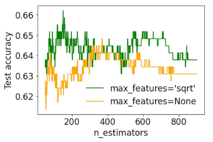
J. Mar. Sci. Eng. 2021, 9, 298                                                                                                  9 of 17

                                 improve the performance of RF models [46]. The seven key hyperparameters
                                                                                                       √       are specified
                                 in Table 2. The usual choices for the hyperparameter max features
                                                                                          √        are   n, log 2 n, and the
                                 number of features n. In this case, n = 35; therefore, n and log2 n would give the
                                 same results.

                                 Table 2. Overview of the different hyperparameters of the standard random forest classifier module.
                                 The number of features is represented by n.

                                         Hyperparameter                         Description                        Default
                                                                     Number of features to consider at                √
                                          max_features                                                                    n
                                                                                each split
                                           n_estimators                Number of trees in the forest                  100
                                            max_depth                  Maximum depth of each tree                 Unlimited
                                                                       Minimum number of samples
                                        min_samples_split                                                              2
                                                                     required to split an internal node
                                                                       Minimum number of samples
                                        min_samples_leaf                                                               1
                                                                       required to be at a leaf node
                                         max_leaf_nodes              Maximum number of leaf nodes                 Unlimited
                                                                    Function to measure the quality of a
                                              criterion                                                              Gini
                                                                           split, Gini, or entropy

                                      One of the simplest and most valuable tuning strategies is grid search, where all
                                 possible combinations of given discrete parameter spaces are evaluated, which was adopted
                                 in this study. The models were implemented using standard libraries from scikit-learn [47].

                                 4. Results
                                      The optimization of RF hyperparameters was the first step of development, following
                                 the workflow described in the last section. Figure 6; Figure 7 show the results, where the
                                 trade-offs between accuracy and different combinations of hyperparameters can be ana-
                                 lyzed, allowing for a loose optimization of the machine learning model. It can be seen
                                 that all parameters except the number of trees tended to overfit very rapidly. The effect
                                 of the number of trees in random forests was studied by [48], who explained that as this
                                 number grows, the performance of the forest is not always better than previous forests with
                                 fewer trees, i.e., a threshold exists, beyond which there is no significant gain. The present
                                 classification between NWW3 and GWES forecasts, through Figure 6, agrees with [48],
                                 where increasing n did not necessarily improve the performance of the RF model.

                                 Figure 6. Test set accuracy as a function of the parameter n_estimators, i.e., the number of trees in
                                                                                                         √
                                 the forest, which was computed with the parameter max_features set to n or None.
J. Mar. Sci. Eng. 2021, 9, 298 10 of 17
Figure 7. Training and test set accuracies as a function of the parameters max_depth, max_leaf_node,
min_sample_split, and min_samples_leaf, presented in the x-axis of each plot. The parameter
max_depth is the maximum depth of each tree, max_leaf_nodes is the maximum leaf nodes in
each tree, min_sample_split is the minimum number of samples required to split an internal node,
and min_samples_leaf is the minimum number of samples required at the leaf node.
Therefore, based on Figures 6 and 7, the initial configuration of the RF model involved
setting the number √ of trees (n_estimators) to 100, the number of features at each split
(max_features) to n (sqrt), the maximum depth of the tree (max_depth) to 10, the min-
imum number of samples required to split an internal node (min_samples_split) to 30,
the maximum leaf nodes (max_leaf_nodes) to 10, and the criterion to “entropy.” The mini-
mum number of samples at a leaf node (min_samples_leaf) was set to 1 due to its correlation
with min_samples_split.
The result of the RFECV method for feature selection using permutation importance,
which required relatively high computational effort, is presented in Figure 8. The features
are ordered from most important to least important, where each bar represents the average
ranking score of the runs, and the numbers at the edge represent the standard deviation of
the ranking score. The rank scores vary from 0 to 1.
The results of Figure 8 respond to the characteristics of NWW3 and GWES, including
the ensemble forecasting compared to the deterministic forecasting. On forecast day 0 (now-
cast), the most important variables included the Hs of GWES, wave direction, the spread of
the ensemble members, and the peak periods. As the nowcast is mostly associated with
better predictions using NWW3 than GWES, it can be seen that the information of the
ensemble spread, together with the ensemble wave height, could help with identifying the
best wave forecast, including the unexpected events when GWES was better than NWW3
in the short range. Moving to forecast days 5 and 7.5, the ranks changed significantly when
entering more complex modeling with lower RF model performances, as is discussed later.
This feature justified the construction of independent RF models, one for each forecast time.
The next step investigated how the accuracy of each RF changed when variables
(listed in Figure 8) were progressively added to the model. The results of multiple runs are
displayed in Figure 9, as well as the mean accuracy of each case. The maximum accuracy
was achieved with nine variables for forecast day 0, with five variables for forecast day 5,
and with four variables for forecast day 7.5. The top mean accuracy of each chosen model
varied with the forecast range, which certainly impacted the feature selection. The nowcastJ. Mar. Sci. Eng. 2021, 9, 298 11 of 17
had the best results with 67.2%, followed by the 5-day forecast (57.0%), and the 7.5-day
forecast (57.1%). The randomness increased while the RF performance decreased with the
forecast time, and thus, the classification was more uncertain with longer forecast ranges.
Figure 8. Final feature importance mean ranking in descending order. The blue colors indicate more
important features for the random forest (RF) model, while the red colors point to less important
variables. The values at the top of each bar correspond to the standard deviation of the feature’s
ranking score. The three forecast times, 0, 5 and 7.5 days are indicated in the plots.
Figure 9. Accuracy of the model as a function of the number of features (n). Each grey dashed line represents a sample,
while the black solid line shows the samples’ average for each n. The three forecast times, 0, 5 and 7.5 days are indicated in
the plots.
A deeper feature analysis was also performed, where the variables that were chosen
were based on the oscillations of the mean accuracy in Figure 9 and the correlation values
between features in Figure 5. The tests were repeated in the same samples that were testedJ. Mar. Sci. Eng. 2021, 9, 298 12 of 17
previously while always looking for the simplest model possible. Going beyond the pure
statistical analysis, the nature of wind-generated ocean waves and how they are simulated
were also taken into account. In forecast day 0, the variables chosen to stay in the RF
model were Hs1, Hs21, sinD0, varHs1, cosD0, sinDs21, cosD1, Tp0, and Tp1. However,
the mean accuracy stayed constant when adding the last two variables. Since they were
highly correlated, only Tp1 was removed at first. Therefore, the information of the wave
height, ensemble spread, wave direction, and period was guaranteed in the RF simulations.
Furthermore, based on the top absolute correlations, additional variables Hw1, Hs10,
sinDw0, cosDw1, sinDs11, Ts11, and cosDs10 were tested for individual insertion into
the model. The results of all tests were either worse or very similar, except for cosDs10,
which resulted in a slight increase in the model accuracy by 0.4%.
For forecast day 5, the variables chosen to stay in the model were sinD0, Hs0, Ts20,
Ts11, and cosDw0. Four of the five features came from NWW3 and, unexpectedly, the in-
formation of the ensemble spread (through the variance of members) was not included by
the feature selection method. A few experiments that involved removing and inserting
some variables were done while looking at the results of Figures 5, 8 and 9. Almost all
individual experiments improved the model accuracy; Tp0 as the variable that contributed
the greatest shift (1%). Adding the combination of Tp0, Hw0, and cosDs21 led to the best
result, and thus, the final choice. This means that the total wave peak period of NWW3,
the wave height of the wind sea of NWW3, and the cosine of the direction of the swell
partition of GWES provide key information for selecting the best wave forecast with a
5-day forecast range.
For forecast day 7.5, the variables chosen to stay in the model were Tw0, cosDw0,
cosDs11, and varHs1. The ensemble spread, quantified by varHs1, did not improve the
model’s accuracy, and thus, it was removed. Considering the top absolute correlations,
the variables that were tested for individual insertion in the model were sinDw0, Hs1, Tp0,
sinD0, and Hs11. Based on the oscillations of the mean accuracy in Figure 9, the variables
cosDw1 and cosDs21 were also included for testing. Removing varHs1 and inserting
Hs1 and Tp0 resulted in the best model, with an improvement of 0.8% in the model
accuracy. Therefore, once again, the ensemble spread did not improve the RF model
accuracy, while the significant wave height of GWES and the peak period of NWW3 were
found to be crucial to the performance of the RF model. The list of the best and final feature
space of the three RF models, one for each forecast time, is summarized in Table 3.
Table 3. Selected features for the final RF models. The full names of variables can be found in Table 1.
Forecast Time (Days) Variables
0 Hs1, Hs21, sinD0, varHs1, cosD0, sinDs21, cosD1, Tp0, cosDs10
5 sinD0, Hs0, Ts20, cosDw0, Tp0, Hw0, cosDs21
7.5 Tw0, cosDw0, cosDs11, Hs1, Tp0
Once the features were defined, the optimization of the hyperparameters could be
performed. The RF model tuning was done using a grid search strategy, which required the
user to determine a range of values for each hyperparameter since the optimal values were
dependent on the dataset at hand. The range of values was chosen based on the analysis of
Figure 7 and they are presented in Table√ 4. Additionally, the parameters with fixed values
were n_estimators (400), max_features ( n), and min_samples_leaf (1).
The final RF models, one per forecast lead time, were run after the fine-tuning. The clas-
sification accuracy results for the training and test sets are given below (respectively), i.e.,
the ability to select the best forecast of Hs between NWW3 and GWES:
(1) Forecast day 0: 0.71, 0.68.
(2) Forecast day 5: 0.65, 0.50.
(3) Forecast day 7.5: 0.63, 0.53.J. Mar. Sci. Eng. 2021, 9, 298 13 of 17
Table 4. Tuning of the hyperparameters.
Hyperparameter Range Searched Forecast Day 0 Forecast Day 5 ForecastDay 7.5
max_depth {2, 15} 4 4 4
min_samples_split {35, 50} 50 40 45
max_leaf_nodes {3, 20} 7 8 5
criterion Gini or entropy Gini Gini Entropy
The accuracy values indicated that the RF model had difficulties in distinguishing
between the two wave predictions. The best results were obtained for the nowcast (day 0),
which, in 70% of cases, the RF model could determine the best forecast. This performance
was worse for forecast days 5 and 7.5, indicating the RF models did not capture a clear
pattern between the feature space and the model that gave a lower Hs error. Therefore,
from the environmental variables selected, it is not evident that NWW3 will certainly have
lower/higher Hs errors under specific metocean conditions than GWES. This result justifies
the importance of providing ensemble forecasts, even at short forecast ranges, despite the
greater advantages of ensemble products over deterministic forecasts occurring beyond a
5-day forecast range. Figure 10 exemplifies the lack of a distinct pattern between the two
most important features when predicting the class. One possible explanation is the fact
that both forecasts were generated with the same numerical wave model (WAVEWATCH
III) and the same physics. If different numerical data and physics had been implemented,
the RF models would probably have more information in the variables to better differentiate
the classes.
Figure 10. Relationship between the two most important features and the target for each dataset
related to the three forecast leads considered. Green points represent the combinations in class 0
(NWW3) and blue points represent the combinations in class 1 (GWES). The three forecast times,
0, 5 and 7.5 days are indicated in the plots.
The best way to examine an RF model’s performance is with confusion matrices of
the results in test sets, as displayed in Figure 11. At this point, the overall accuracy of
each RF model presented above could be further analyzed through false and true RF
predictions of the best wave forecast, including the two classes. Note that the classes have
different counts and percentages, as presented in Figure 4, which can be quantified using
Figure 11 by looking at each column of the plots. The RF model for forecast day 0 correctly
predicted NWW3 being the best wave forecast in 59.51% of the cases, with false predictions
of GWES as the best wave forecast in only 1.46%. This is a reasonably good accuracy of the
RF; however, it must be balanced by the 30.73% of false predictions of GWES providing
the best forecast. Considering that NWW3 is usually better than GWES for nowcasts,
correctly determining when GWES is better than NWW3 is a great challenge, which was
correctly classified by the RF model in 8.29% of cases.J. Mar. Sci. Eng. 2021, 9, 298 14 of 17
Figure 11. Confusion matrices showing the percentage of data in each position, where class 0 refers to NWW3 and class 1
refers to GWES. The positions are true 0 (correctly classifying class 0), false 1 (falsely classifying as class 1), false 0 (falsely
classifying as class 0), and true 1 (correctly classifying class 1). The three plots are associated with the forecast lead times:
day 0 (left), day 5 (center), and day 7.5 (right), indicated in the plots.
For forecast day 5, the RF model quality deteriorated. The false RF predictions
choosing NWW3 as the best model reached 36.8%, which is too high for such modeling.
This means that 36.8% of the time, the RF model should have identified that GWES was
the best wave forecast but it erroneously classified it as NWW3. The forecast day 5
represents the worst accuracy of the RF model among the three forecast ranges analyzed,
which probably resulted from the combination of similar performances of NWW3 and
GWES (Figures 3 and 4), with no clear pattern of input variables linked to the Hs forecast
errors (Figure 10).
For forecast day 7.5, the RF model correctly pointed to GWES as the best wave forecast
in 33.0% of cases but it mispredicted GWES as being the best model in 28.0% of cases,
which is a strong limitation of the machine learning classification. Once again, the skill of
the RF model was poor, with 19.5% showing true NWW3 and the same 19.5% showing false
NWW3, meaning that the RF model was not able to properly select the best wave forecast
with a one-week forecast horizon. The joint analysis of the three confusion matrices in
Figure 11 indicated that the RF models were better predictors of the class with the largest
count in the dataset, as expected; i.e., true NWW3 in the nowcast and true GWES on
day 7.5. It would be ideal to predict true GWES and true NWW3 in the nowcast and
day 7.5, respectively. However, the RF models developed showed a minor accuracy for
those conditions.
5. Conclusions
This study introduced a case of postprocessing random forest (RF) modeling, which is
a supervised learning classifier, to identify the best wave prediction between two wave
forecasts available, namely, the deterministic NWW3 and the ensemble mean of GWES,
involving forecast ranges from 0 to 7.5 days. The criterion used established the best model
as the one with the lowest significant wave height (Hs) error. A total of 35 environmental
variables were investigated to compose the feature space for the RF model input, including
wind speed, wave height, period, and direction, as well as wind sea and swell partitions.
The RF model was trained using quality-controlled data from five NDBC buoys.
Significant effort was invested into examining the impact of each variable on the
RF model accuracy, using RFE and permutation importance as a first step, and later,
by manually including or excluding the most relevant variables. The information of the
total wave height, wave direction (especially swell), and wave period were crucial for
improving the RF model’s performance. Additionally, the ensemble spread of Hs was found
to be relevant to the short-term forecast classification. In ensemble forecasting, the spread
tends to increase with the forecast lead time, as well as under extreme conditions associated
with large uncertainties. For short-term forecasts, the spread is usually very small; however,
certain metocean conditions that are more difficult to predict often become associated with
increasing spread. This study showed that the RF model captured this behavior through
the variance of the ensemble members to improve the decision between NWW3 and GWES.J. Mar. Sci. Eng. 2021, 9, 298 15 of 17
This was successful for the short-term predictions for the first forecast day, but it did not
contribute to the RF model for forecast day 5 and beyond, possibly due to the intrinsic
larger spread that was already present at these forecast horizons.
The overall accuracies (test set) of the RF models were 67.8%, 50.2%, and 52.5% in
datasets with predictions from forecast days 0, 5, and 7.5, respectively. These results,
together with the confusion matrices (Figure 11), suggest that the RF models developed
were able to support the decision between NWW3 and GWES for short-term forecasts, only.
Moving to 5-day and one-week forecasts, the RF models did not find enough information
in the feature space to successfully determine the best wave forecast (the lowest Hs error).
The increased entropy in the system with longer forecast leads and the large spread of
values added complexity to the classification, and thus, compromised the RF performance.
Using larger datasets, by including long reforecast simulations and satellite observations,
as well as expanding the approach to other classifiers, such as those described by [41],
could improve the decision between wave predictions in future studies.
Author Contributions: Conceptualization, R.M.C.; methodology, R.M.C. and M.O.C.; formal analy-
sis, M.O.C.; data processing, R.M.C., F.A., and M.O.C.; writing—original draft preparation, R.M.C.
and M.O.C.; writing—review and editing, C.G.S.; visualization, M.O.C., F.A., and R.M.C.; supervision,
C.G.S. All authors have read and agreed to the published version of the manuscript.
Funding: This work was conducted within the project WAVEFAI—Operational Wave Forecast using
Artificial Intelligence, which is funded by the Portuguese Foundation for Science and Technology
(Fundação para a Ciência e Tecnologia (FCT)) under the contract 1801P.01023. This work contributes
to the Strategic Research Plan of the Centre for Marine Technology and Ocean Engineering (CENTEC),
which is financed by FCT under contract UIDB/UIDP/00134/2020.
Institutional Review Board Statement: Not applicable.
Informed Consent Statement: Not applicable.
Data Availability Statement: The forecast data and buoy data can be obtained in the links: https:
//www.ftp.ncep.noaa.gov/data/nccf/com/wave/prod/ (accessed on 1 November 2020), http:
//www.ndbc.noaa.gov/ (accessed on 1 November 2020).
Acknowledgments: The authors acknowledge the National Centers for Environmental Prediction
(NCEP/NOAA) and the National Data Buoy Center (NDBC/NOAA) for providing the forecast and
buoy data.
Conflicts of Interest: The authors declare no conflict of interest.
References
1. Hinnenthal, J.; Clauss, G. Robust Pareto-optimum routing of ships utilizing deterministic and ensemble weather forecasts. Ships
Offshore Struct. 2010, 5, 105–114. [CrossRef]
2. Vettor, R.; Guedes Soares, C. Development of a ship weather routing system. Ocean Eng. 2016, 123, 1–14. [CrossRef]
3. Perera, L.P.; Guedes Soares, C. Weather Routing and Safe Ship Handling in the Future of Shipping. Ocean Eng. 2017, 130, 684–695.
[CrossRef]
4. Fu, T.; Babanin, A.; Bentamy, A.; Campos, R.; Dong, S.; Gramstad, O.; Kapsenberg, G.; Mao, W.; Miyake, R.; Murphy, A.J.
Committee No I.1: Environment. In Proceedings of the 20th International Ship and Offshore Structures Congress, Liege, Belgium,
9–14 September 2018; pp. 9–13.
5. Laface, V.; Arena, F.; Guedes Soares, C. Directional analysis of sea storms. Ocean Eng. 2015, 107, 45–53. [CrossRef]
6. de Leon, S.P.; Guedes Soares, C. Extreme wave parameters under North Atlantic extratropical cyclones. Ocean Model. 2014, 81,
78–88. [CrossRef]
7. Campos, R.M.; Alves, J.H.G.M.; Guedes Soares, C.; Guimaraes, L.G.; Parente, C.E. Extreme wind-wave modeling and analysis in
the south Atlantic ocean. Ocean Model. 2018, 124, 75–93. [CrossRef]
8. Gramcianinov, C.B.; Campos, R.M.; Camargo, R.; Hodges, K.I.; Guedes Soares, C.; Silva Dias, P.L. Analysis of Atlantic extratropical
storm tracks characteristics in 41 years of ERA5 and CFSR/CFSv2 Databases. Ocean Eng. 2020, 216, 108111. [CrossRef]
9. Gramcianinov, C.B.; Campos, R.M.; Guedes Soares, C.; Camargo, R. Extreme waves generated by cyclonic winds in the western
portion of the South Atlantic Ocean. Ocean Eng. 2020, 213, 107745. [CrossRef]
10. Cavaleri, L.; Alves, J.H.G.M.; Ardhuin, F.; Babanin, A.; Banner, M.; Belibassakis, K.; Benoit, M.; Donelan, M.; Groeneweg, J.;
Herbers, T.H.C.; et al. Wave modelling—The state of the art. Prog. Oceanogr. 2007, 75, 603–674. [CrossRef]J. Mar. Sci. Eng. 2021, 9, 298 16 of 17
11. Campos, R.M.; Alves, J.H.G.M.; Penny, S.G.; Krasnopolsky, V. Assessments of surface winds and waves from the NCEP Ensemble
Forecast System. Weather Forecast. 2018, 33, 1533–1564. [CrossRef]
12. Lorenz, E.N. A Study of the Predictability of a 28-Variable Atmospheric Model. Tellus 1965, 17, 321–333. [CrossRef]
13. Lorenz, E.N. The Nature and Theory of the General Circulation of the Atmosphere; World Meteorological Organization: Geneva,
Switzerland, 1967.
14. Chen, H.S. Ensemble prediction of ocean waves at NCEP. In Proceedings of the 28th Ocean Engineering Conference, Kaohsiung,
Taiwan, November 2006.
15. Cao, D.; Chen, H.S.; Tolman, H. Verification of ocean wave ensemble forecasts at NCEP. In Proceedings of the 10th International
Workshop on Wave Hindcasting and Forecasting and First Coastal Hazards Symposium, Camp Springs, MD, USA, 11–16
November 2007.
16. Campos, R.M.; Alves, J.H.G.M.; Penny, S.G.; Krasnopolsky, V. Global assessments of the NCEP Ensemble Forecast System using
altimeter data. Ocean Dyn. 2020, 70, 405–419. [CrossRef]
17. Alves, J.H.G.M.; Wittman, P.; Sestak, M.; Schauer, J.; Stripling, S.; Bernier, N.B.; McLean, J.; Chao, Y.; Chawla, A.; Tolman, H.; et al.
The NCEP–FNMOC combined wave ensemble product. Expanding benefits of interagency probabilistic forecasts to the oceanic
environment. Bull. Am. Meteorol. Soc. BAMS 2013, 94, 1893–1905. [CrossRef]
18. Bidlot, J.R. Twenty-one years of wave forecast verification. ECMWF Newsl. 2017, 150, 31–36. Available online: https://www.
ecmwf.int/node/18165 (accessed on 1 November 2020).
19. Deo, M.C.; Jha, A.; Chaphekar, A.S.; Ravikant, K. Neural networks for wave forecasting. Ocean Eng. 2001, 28, 889–898. [CrossRef]
20. Makarynskyy, O.; Pires-Silva, A.A.; Makarynska, D.; Ventura-Soares, C. Artificial neural networks in wave predictions at the west
coast of Portugal. Comput. Geosci. 2005, 31, 415–424. [CrossRef]
21. Jain, P.; Deo, M.C. Neural networks in ocean engineering. Ships Offshore Struct. 2006, 1, 25–35. [CrossRef]
22. Kumar, N.K.; Savitha, R.; Al Mamun, A. Regional ocean wave height prediction using sequential learning neural networks. Ocean
Eng. 2017, 129, 605–612. [CrossRef]
23. Campos, R.M.; Krasnopolsky, V.; Alves, J.H.G.M.; Penny, S.G. Improving NCEP’s global-scale wave ensemble averages using
neural networks. Ocean Model. 2020, 149, 101617. [CrossRef]
24. Deka, P.C.; Prahlada, R. Discrete wavelet neural network approach in significant wave height forecasting for multistep lead time.
Ocean Eng. 2012, 43, 32–42. [CrossRef]
25. Dixit, P.; Londhe, S. Prediction of extreme wave heights using neuro wavelet technique. Appl. Ocean Res. 2016, 58, 241–252.
[CrossRef]
26. Oh, J.; Suh, K.-D. Real-time forecasting of wave heights using EOF-wavelet-neural network hybrid model. Ocean Eng. 2018, 150,
48–59. [CrossRef]
27. Berbić, J.; Ocvirk, E.; Carević, D.; Lončar, G. Application of neural networks and support vector machine for significant wave
height prediction. Oceanologia 2017, 59, 331–349. [CrossRef]
28. Mahjoobi, J.; Etemad-Shahidi, A. An alternative approach for the prediction of significant wave heights based on classification
and regression trees. Appl. Ocean Res. 2008, 30, 172–177. [CrossRef]
29. Callens, A.; Morichon, D.; Abadie, S.; Delpey, M.; Liquet, B. Using random forest and gradient boosting trees to improve wave
forecast at a specific location. Appl. Ocean Res. 2020, 104, 102339. [CrossRef]
30. Campos, R.M.; Guedes Soares, C. Comparison and assessment of three wave hindcasts in the North Atlantic Ocean. J. Oper.
Oceanogr. 2016, 9, 26–44. [CrossRef]
31. Stopa, J.E.; Cheung, K.F. Intercomparison of wind and wave data from the ECMWF Reanalysis Interim and the NCEP Climate
Forecast System Reanalysis. Ocean Model. 2014, 75, 65–83. [CrossRef]
32. Zhou, X.; Zhu, Y.; Hou, D.; Luo, Y.; Peng, J.; Wobus, R. Performance of the new NCEP global ensemble forecast system in a
parallel experiment. Weather Forecast. 2017, 32, 1989–2004. [CrossRef]
33. Tolman, H.; Accensi, M.; Alves, J.H.; Ardhuin, F.; Bidlot, J.; Booij, N.; Bennis, A.C.; Campbell, T.; Chalikov, D.; Chawla, A. User
manual and System Documentation of WAVEWATCH III R Version; NOAA/NWS/NCEP/MMAB: Baltimore, MD, USA, 2019; 465p.
34. Ardhuin, F.; Rogers, E.; Babanin, A.V.; Filipot, J.; Magne, R.; Roland, A.; Westhuysen, A.; Queffeulou, P.; Lefevre, J.; Aouf, L.; et al.
Semiempirical dissipation source functions for ocean waves. Part I: Definition, calibration, and validation. J. Phys. Oceanogr. 2010,
40, 1917–1941. [CrossRef]
35. Jolliff, J.K.; Kindle, J.C.; Shulman, I.; Penta, B.; Friedrichs, M.A.M.; Helber, R.; Arnone, R.A. Summary diagrams for coupled
hydrodynamic-ecosystem model skill assessment. J. Mar. Syst. 2009, 76, 64–82. [CrossRef]
36. Khaire, U.M.; Dhanalakshmi, R.; Stability of feature selection algorithm: A review. J. King Saud Univ. Comput. Inf. Sci. 2019.
Available online: https://www.sciencedirect.com/science/article/pii/S1319157819304379 (accessed on 1 November 2020).
37. Breiman, L.; Friedman, J.; Stone, C.J.; Olshen, R.A. Classification and Regression Trees; CRC Press: Boca Raton, FL, USA, 1984.
38. Strobl, C.; Boulesteix, A.-L.; Zeileis, A.; Hothorn, T. Bias in random forest variable importance measures: Illustrations, sources
and a solution. BMC Bioinform. 2007, 8, 25. [CrossRef] [PubMed]
39. Breiman, L. Random forests. Mach. Learn. 2001, 45, 5–32. [CrossRef]
40. Guyon, I.; Weston, J.; Barnhill, S.; Vapnik, V. Gene selection for cancer classification using support vector machines. Mach. Learn.
2002, 46, 389–422. [CrossRef]J. Mar. Sci. Eng. 2021, 9, 298 17 of 17
41. Parr, T.; Turgutlu, K.; Csiszar, C.; Howard, J. Beware Default Random Forest Importances. Explained.ai. 2018. Available online:
https://explained.ai/rf-importance/ (accessed on 1 November 2020).
42. Gregorutti, B.; Michel, B.; Saint-Pierre, P. Correlation and variable importance in random forests. Stat. Comput. 2017, 27, 659–678.
[CrossRef]
43. Zaki, M.J.; Meira, W. Data Mining and Machine Learning: Fundamental Concepts and Algorithms; Cambridge University Press:
Cambridge, UK, 2020.
44. Friedman, J.; Hastie, T.; Tibshirani, R. The Elements of Statistical Learning; Springer: New York, NY, USA, 2009.
45. Witten, I.H.; Frank, E. Data mining: Practical machine learning tools and techniques with java implementations. ACM Sigmod.
Record 2002, 31, 76–77. [CrossRef]
46. Probst, P.; Wright, M.N.; Boulesteix, A.-L. Hyperparameters and tuning strategies for random forest. Wiley Interdiscip. Rev. Data
Min. Knowl. Discov. 2019, 9, 1301. [CrossRef]
47. Pedregosa, F.; Varoquaux, G.; Gramfort, A.; Michel, V.; Thirion, B.; Grisel, O.; Blondel, M.; Prettenhofer, P.; Weiss, R.; Dubourg, V.
Scikit-learn: Machine learning in python. J. Mach. Learn. Res. 2011, 12, 2825–2830.
48. Oshiro, T.M.; Perez, P.S.; Baranauskas, J.A. How many Trees in a Random Forest? International Workshop on Machine Learning and Data
Mining in Pattern Recognition; Springer: Berlin/Heidelberg, Germany, 2012; pp. 154–168.You can also read