Kokkinakis, Ioannis W. and Drikakis, Dimitris and Youngs, David L. (2019) Modeling of Rayleigh-Taylor mixing using single-fluid models. Physical ...
←
→
Page content transcription
If your browser does not render page correctly, please read the page content below
Kokkinakis, Ioannis W. and Drikakis, Dimitris and Youngs, David L.
(2019) Modeling of Rayleigh-Taylor mixing using single-fluid models.
Physical Review E, 99 (1). ISSN 2470-0045 ,
http://dx.doi.org/10.1103/PhysRevE.99.013104
This version is available at https://strathprints.strath.ac.uk/67031/
Strathprints is designed to allow users to access the research output of the University of
Strathclyde. Unless otherwise explicitly stated on the manuscript, Copyright © and Moral Rights
for the papers on this site are retained by the individual authors and/or other copyright owners.
Please check the manuscript for details of any other licences that may have been applied. You
may not engage in further distribution of the material for any profitmaking activities or any
commercial gain. You may freely distribute both the url (https://strathprints.strath.ac.uk/) and the
content of this paper for research or private study, educational, or not-for-profit purposes without
prior permission or charge.
Any correspondence concerning this service should be sent to the Strathprints administrator:
strathprints@strath.ac.uk

The Strathprints institutional repository (https://strathprints.strath.ac.uk) is a digital archive of University of Strathclyde research
outputs. It has been developed to disseminate open access research outputs, expose data about those outputs, and enable the
                              management and persistent access to Strathclyde's intellectual output.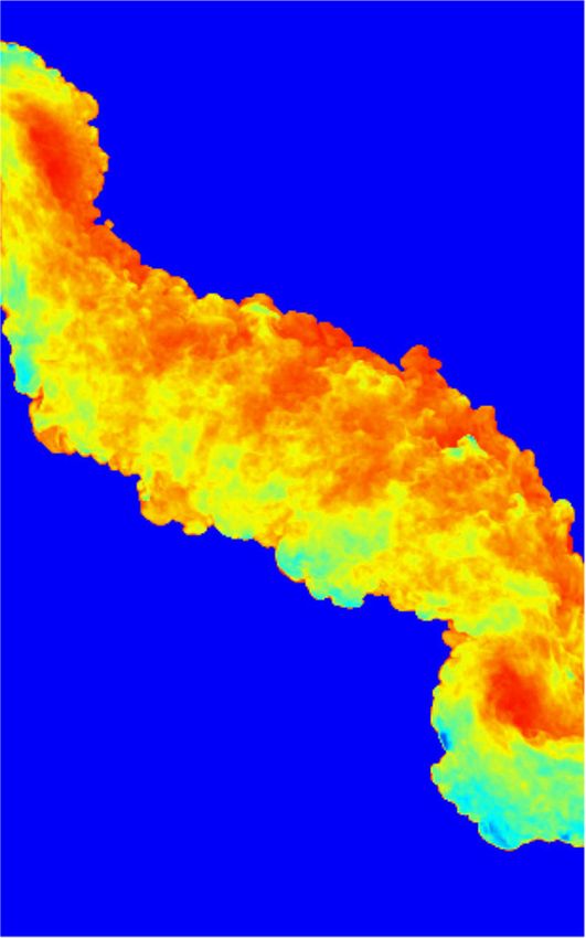
Modeling of Rayleigh–Taylor mixing using single-fluid models

            Ioannis W. Kokkinakis,1 Dimitris Drikakis,2 and David L. Youngs1
                   1
                       University of Strathclyde, Glasgow, United Kingdom
                            2
                                University of Nicosia, Nicosia, Cyprus
                                     (Dated: December 17, 2018)

                                             Abstract
  Turbulence mixing models of different degree of complexity are investigated for Rayleigh–Taylor
mixing flows with reference to high-resolution implicit large eddy simulations. The models consid-
ered, in order of increasing complexity, comprise of the (i) two-equation K-L, (ii) three-equation
K-L-a, (iii) four-equation K-L-a-b, and (iv) Besnard-Harlow-Rauenzahn (BHR-2). The above mod-
els are implemented in the same numerical framework to minimize the computational uncertainty.
The impact of the various approximations represented by the different models is investigated for
canonical 1D Rayleigh–Taylor mixing and for the more complex (2D on average) case of the tilted-
rig experiment, aiming to understand the balance between accuracy and complexity. The results
provide guidance on the relative merits of various turbulence models over a variety of conditions.

                                                1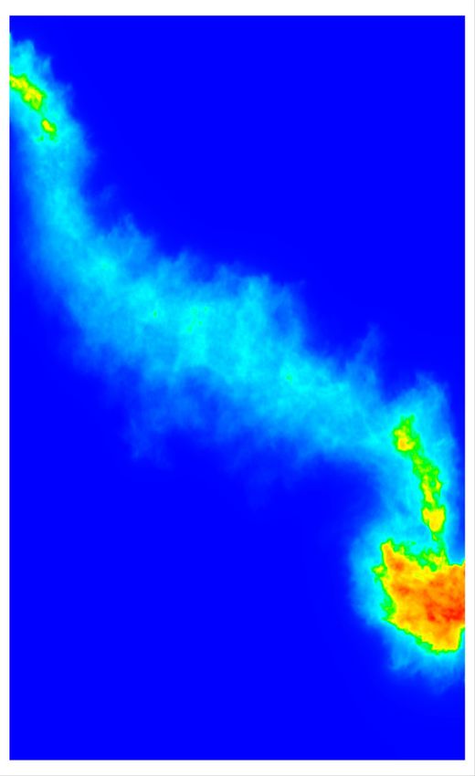
I.    INTRODUCTION

     The Rayleigh–Taylor (RT) instability occurs in a wide range of variable-density flows,
both natural and man-made, including inertial confinement fusion (ICF) [1, 2], cavitation
[3], combustion [4], astrophysics [5–8], and geophysical flows [9].
     Although significant progress has been made in understanding RT mixing by using differ-
ent simulation approaches, including Direct Numerical Simulation (DNS) and Large Eddy
Simulation (LES), these approaches remain computationally expensive for complex applica-
tions such as ICF at high Reynolds numbers [10–22]. For complex applications, turbulence
models based on transport equations, which predict the “average” behavior of the turbu-
lent mixing zone, are employed. Turbulence models allow for larger time steps and coarser
computational grids than DNS and LES. Furthermore, for cases where the average behavior
has homogeneous directions, the computational cost can be further reduced by perform-
ing calculations in preferential directions. Due to the ensemble averaging of the second
and higher-order correlations of turbulent fluctuations, additional terms arise that require
to be modeled. The modeling assumptions and closure coefficients are validated and cali-
brated through comparisons with experiments, but increasingly through comparisons with
high-resolution simulations because quantitative experimental data is limited.
     Turbulence mixing models can be classified into three categories. The simplest models
are called buoyancy drag models [23–26] and use ordinary differential equations to evolve the
width of the mixing layer. The bubble, or spike amplitudes, are described by balancing the
inertia, buoyancy and drag forces. These models cannot model multiple mixing interfaces;
cannot be easily extended to two and three dimensions; and, as a rule, do not address
demixing, also known as counter-gradient transport, i.e., reduction of total fluid masses
within the mixing zone. To address the above problems, two-fluid (or multi-fluid) models
have been proposed [27–30]. They use a separate set of equations for each fluid in addition
to the main flow equations, and provide an accurate modeling framework for demixing by
correctly capturing the relative motion of the different fluid fragments. An intermediate
class of models are the single-fluid models [31–34]. They consist of evolutionary equations
for the turbulence kinetic energy and its dissipation rate, or equivalent turbulence length
scale.
     A more advanced version of the single-fluid models is the Besnard-Harlow-Rauenzahn

                                             2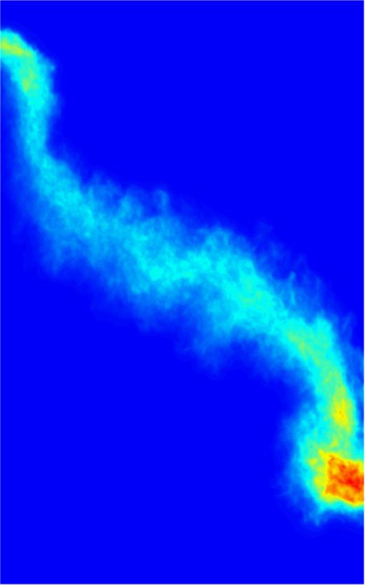
(BHR) model [35]. The BHR model is based on the evolution equations arising from
second-order correlations and gradient-diffusion approximations. Using a mass weighted
averaged decomposition, the original BHR model includes full transport equations for the
Reynolds stresses, turbulent mass-flux velocity, density fluctuations and the turbulence ki-
netic energy dissipation rate. Several efforts were made to simplify the resulting equations.
A three-equation variant was proposed for RT, Kelvin–Helmholtz (KH), and Richtmyer–
Meshkov (RM) flows [36]. A second-moment closure implementation was also presented by
Schwarzkopf et al. [37]. In the present study, the four-equation variant, known as the BHR-2
model [38], was employed. The BHR-2 model is also investigated here in conjunction with
the modified species turbulent diffusion term [39], which can improve accuracy in demixing.
      Despite the aforementioned efforts, there is still an uncertainty over the optimum choice
of turbulence models, a lack of systematic comparison between the different models, as well
as room for significantly improving the models accuracy across flow regimes. In this study,
specific modifications to the original models that result in improved accuracy are proposed.
A systematic comparison of the accuracy of the different models is presented for canonical
planar RT flows [16, 18] and the tilted-rig experiment [27, 40].

II.     TURBULENCE MIXING MODELS

      The first step for the development of turbulence models is to perform Reynolds averaging
of the governing equations and Favre-averaging of the resultant terms. As in previous studies
[27–29, 31, 32, 36, 38], high Reynolds number applications are considered where turbulent
viscosity, conductivity and diffusivity are large compared to molecular values.
      The resulting modeled governing equations of the mixture are given by:

                                             ∂ ρ̄ ∂ ρ̄ũj
                                                 +        =0                                (1)
                                             ∂t    ∂xj

                             ∂ ρ̄ũi    ∂                         ∂τij
                                     +     (ρ̄ũi ũj + p̄δij ) =      + ρ̄gj               (2)
                              ∂t       ∂xj                        ∂xj

                             ∂ ρ̄Ẽ     ∂ ρ̄Ẽ + p̄ ũj∂τij ũi
                                    +                     =     + ρ̄ũj gj
                              ∂t             ∂xj        ∂xj
                                                                        !                   (3)
                                                 ∂qj   ∂       µt ∂K
                                               −     +
                                                 ∂xj ∂xj NK ∂xj

                                                   3
∂ ρ̄F̃ ∂ ρ̄F̃ ũj ∂Jj
+ =− , (4)
∂t ∂xj ∂xj
where variables labeled by “bar” and “tilde” denote Reynolds and Favre averages, respec-
tively; ρ is the density; ui are the velocity components; F is the mass-fraction; and E is the
total energy. The repeated index j implies summation over the dimensions (i, j) = 1, 2, 3;
gj is an external acceleration in the direction of dimension j; and µt is the eddy viscosity.
The perfect gas assumption is employed, p̄ = ρ̄R∗ T̃ , where R∗ is the mixture specific gas
constant and T̃ is the Favre-averaged static temperature corresponding to the static pressure
(conditions) of the mixture.
The Favre-averaged total energy is obtained from the sum of the Favre-averaged internal
energy, kinetic energy, turbulence kinetic energy and potential energy:
ũk ũk
Ẽ = ẽ + + K + gj xj , (5)
2
where ẽ = p̄/ (γ − 1) ρ̄ is the Favre-averaged internal energy per unit mass.
Using the isobaric assumption for the thermodynamic closure of the mixture [41], the
heat capacity ratio of the mixture γ is calculated by:
1
γ =1+ N
, (6)
P fn
γn −1
n=1
where N is the total number of the species and γn is the heat capacity ratio of a component
n. The volume fraction of species n, fn , is calculated by:
Fn /Mn
fn = N
, (7)
Fm /Mm
P
m=1
PN
where Fn and Mn are its mass fraction and molar mass, respectively, and m=1 fm = 1.
The turbulent diffusion terms are adjusted using dimensionless scaling factors such that
Nh and NF correspond to the turbulent Prandtl (P rt = cp µt /κt ) and Schmidt (Sct =
µt /(ρDt ) numbers, respectively. Note that the turbulent transport (diffusion) of the turbu-
lence kinetic energy is also accounted for in Eq. (3).
There are also extra terms arising from the Favre-averaging that need to be modeled: (i)
the Reynolds stress tensor τij ≡ −ρu′′i u′′j , (ii) the turbulent viscosity µt , and (iii) the density
weighted turbulence kinetic energy K ≡ k̃ = u ] u /2 = ρu′′ u′′ /2ρ̄ = −τii /2ρ̄.
′′ ′′
k k k k
4The transport equation for the Favre-averaged turbulence kinetic energy is given by:
∂ ρ̄K ∂ ρ̄K ũj ∂ ũi
+ = SK + τij
∂t ∂xj ∂xj
! (8)
∂ µt ∂K
+ − ρ̄ε ,
∂xj NK ∂xj
where NK is the scaling factor for the turbulence kinetic energy diffusion and ε is the
dissipation:
ε = CD u3t /L . (9)
√
CD is the drag coefficient and ut = 2K is the turbulent velocity. Eq. (8) varies across
models depending on the formulation of the turbulence kinetic energy production source
term, SK .
For the turbulent transport terms in the mass-fraction and total energy equations, the
diffusivities of all species are assumed to be the same [42]. Assuming Fickian diffusion, the
turbulent mass flux of species n is given by:
µt ∂ F̃n
Jn,j = − (10)
NF ∂xj
and for the case of two fluids:
µt ∂ F̃
Jj ≡ J1,j = −J2,j = − (11)
NF ∂xj
The internal energy flux, qj , [43, 44] is obtained from adding the inter-diffusional enthalpy
flux:
N
qjd =
X
h̃n Jn,j , (12)
n=1
where h̃n is the specific enthalpy of species n; and the turbulent heat conduction flux, qjc :
∂ T̃
qjc = −ρ̄DT cp , (13)
∂xj
where cp is the mixture’s specific heat capacity at constant pressure:
N
X
cp = cpn Fn
n=1
If the heat conductivity, DT , is set equal to the species turbulent diffusivity, µt / (ρ̄NF ),
and the fluid species have constant specific heats, the internal energy flux is simplified (see
Kokkinakis et al. [42]) as
µt ∂ h̃
qj = qjd + qjc = − , (14)
NF ∂xj
5where h̃ = γẽ is the Favre-averaged specific enthalpy of the mixture. Equations (11) and
(14) are used in the averaged governing equations of the species mass-fraction (4) and total
energy, (3), respectively.
The set of equations is completed by an equation for the turbulence length scale, L ≡
CD K 3/2 /ε [37]:
∂ ρ̄L ∂ ρ̄Lũj ∂ ũj
=− + CL ρut + CC ρ̄L
∂t ∂xj ∂xj
! (15)
∂ µt ∂L
+ ,
∂xj NL ∂xj
where on the right-hand-side (RHS) the second, third and last term are used to model
production, compressibility effects, and turbulent diffusion, respectively, where CL =1 and
CC =1/3. The rest of the model constants are given in the Appendix.
The eddy viscosity is calculated by:
µt = Cµ ρ̄ut L , (16)
where Cµ is a constant.
All turbulence mixing models are calibrated using the full Reynolds stress tensor based
on the Boussinesq eddy-viscosity assumption:
!
∂ ũj ∂ ũi 1 ∂ ũk 2
τij = µt + − δij − ρ̄Kδij . (17)
∂xi ∂xj 3 ∂xk 3
A. K-L model
The K-L model was proposed by Dimonte and Tipton [32] for describing the turbulent
self-similar regime of RT and RM induced mixing. The starting point for deriving the
model equations are the buoyancy-drag models for the self-similar growth of RT and RM
instabilities [23, 25]. Here, an improved version of the model proposed by Kokkinakis et al.
[42] is used based on the following modifications: (i) a transport equation for the total energy,
Eq. (3), instead of the internal energy; (ii) the turbulent diffusion of specific enthalpy instead
of internal energy in Eq. (3); (iii) the implementation of the source term (SK ) in Eq. (8)
based on the mean flow and turbulence time-scales; and (iv) the calculation of the local
Atwood number based on higher-order numerical approximations.
6B. K-L-a model
The three-equation model of Morgan and Wickett [45] was developed as an extension to
the two-equation K-L model of Dimonte and Tipton [32] by including a third equation for
the turbulent mass-flux velocity, ai ≡ ρ′ u′i /ρ̄ = −u′′i .
The production source term of the turbulence kinetic energy is given by
∂ p̄
SK = CB aj , (18)
∂xj
and the governing equation for the mass-flux velocity is written as
∂ ρ̄ai ∂ ρ̄ũj ai ∂ p̄ τij ∂ ρ̄
=− +b +
∂t ∂xj ∂xi ρ̄ ∂xj
! (19)
∂ µt ∂ai ut
+ − CDa ρ̄ai .
∂xj Na ∂xj L
The density-specific volume covariance b ≡ −ρ′ (1/ρ)′ , is a (positive) measure of the
molecular mixing state of the mixture. An algebraic expression generalized for an n-
component mixture and includes an added-mass correction factor, c, is [45]:
P fn
n ρn +cρ̄
b= ρ̄ P fn ρn −1, (20)
n ρn +cρ̄
where c is determined from the iLES. For perfectly molecularly mixed fluids b = 0, whereas
for two immiscible fluids, b attains a maximum value given by a simple two-fluid formulation
[36]:
(ρ1 − ρ2 )2
b = f1 f2 , (21)
ρ1 ρ2
where f1 and f2 are the volume fractions associated with the fluids composing the binary
mixture and can be obtained by setting c = 0 in Eq. (20). Positive values of c allow for some
adjustment to the maximum value of b. No miscible fluids formulation for the algebraic
estimation of b, nor the added-mass correction factor, c, is known.
Morgan et al. [46] have recently extended the K-L-a model to include a second length
scale equation, which relies on separating the turbulence transport (Lt ≡ L) and turbulence
destruction (Ld ) length scales. This is similar to the work carried out by Schwarzkopf
et al. [47] for the BHR-3.1 model. The two-length-scale approach is necessary in order to
simultaneously capture the growth parameter and turbulence intensity of a Kelvin-Helmholtz
shear layer when model coefficients are constrained by similarity analysis.
7C. K-L-a-b model
We have extended here the K-L-a model by adding an evolution equation for the density-
specific volume covariance (b). Examining Eq. (19) shows that b governs the primary produc-
tion mechanism of the turbulent mass-flux and, therefore, needs to be modeled accurately
to reflect the effects of the changes in the density fluctuations [38].
The governing equation for b employed here is similar to the BHR-2 model [38, 48, 49],
but with the redistribution term omitted, as per Morgan and Wickett [45] with respect to a
in Eq. (19):
∂ ρ̄b ∂ ρ̄ũj b ∂ ρ̄
=− − 2 (b + 1) aj
∂t ∂xj ∂xj
! (22)
∂ µt ∂b ut
+ρ̄2 2
− CDb b ,
∂xj ρ̄ σb ∂xj L
where the remaining terms on the right hand side (RHS) are the advection, production,
turbulent diffusion, and destruction terms, respectively. The K-L-a-b is essentially a reduced
form of the BHR-2 model presented in the next section.
D. BHR-2 model
The basic formulation for the BHR model can be found in the paper by Besnard et al. [48]
but several variants have also been proposed. The BHR-2 variant, considered in this study,
uses an algebraic closure for the Reynolds stresses, and the gradient diffusion approximation
for the turbulent fluxes. An extensive review of the BHR-2 model can be found in [38, 49, 50].
The model introduces several additional terms in the governing equations of the turbulence
length scale (L), turbulent mass-flux velocity (ai ) and density-specific volume covariance
(b).
For the turbulence length scale, the model omits the compression term, but adds two
additional terms associated with net production:
∂ ρ̄L ∂ ũj
= RHS[of (15)] − CC ρ̄L
∂t ∂xj
" ! !# (23)
L ∂ p̄ ∂ ũi
+ CL4 aj + CL1 τij ,
K ∂xj ∂xj
where CL4 = (3/2 − C4 ) and CL1 = (3/2 − C1 ).
8For the turbulent mass-flux velocity, an additional production term and a redistribution
term are included:
∂ ρ̄ai
= RHS[of (19)]
∂t
∂(ũi − ai ) ∂ai aj (24)
−CBa ρ̄aj + CRa ρ̄
∂xj ∂xj
Finally, a redistribution term is also included for the density-specific-volume covariance:
∂ ρ̄b ∂b
= RHS[of (22)] + 2CRb ρ̄aj (25)
∂t ∂xj
In this study, the model is implemented in conjunction with the total energy (Ẽ) instead
of the specific internal energy (ẽ). This is similar to the BHR-3 model [37, 48] and its two-
length scale variant BHR-3.1 [47]. Using the same equation for Ẽ for all turbulence models
considered here, allows for a more meaningful and direct comparison between the different
turbulence models to be carried out.
The gradient diffusion approximation (GDA) is typically used to model the turbulent
transport terms; for the species mass-fraction it is defined as:
!
∂ ′′ ′′ ∂ µt ∂ F̃
− ρuj F = . (26)
∂xj ∂xj NF ∂xj
Bertsch and Gore [39] developed a modified species turbulent diffusion (MSTD) term and
applied it in the framework of the second moment closure BHR-3.1 model. MSTD enables
counter gradient transport and can model demixing in both BHR-3 and BHR-3.1 models.
According to [39], the turbulent transport term on the RHS of Eq. (4) can be formulated in
the incompressible limit as:
!
∂ ′′ ′′ ρ1 ρ2 ∂aj
− ρuj F = , (27)
∂xj ρ2 − ρ1 ∂xj
MSTD requires the turbulent mass-flux velocity (ai ) and partial densities, therefore, it can
be implemented in any model that includes a transport equation for ai . Results for the
BHR-2 model using the MSTD, as well as the GDA (with and without the SF limiter), are
shown in relation to the tilted rig case only because the results were identical for the 1D
problem.
9E. Implementation details
The realizability conditions of Vreman et al. [51] are imposed on the Reynolds stresses:
τii ≤ 0 , |τij | ≤ (τii τjj ) /2
1
(28)
det (τij ) ≥ 0 , |τij | ≤ 2ρ̄K ,
where the Reynolds stress tensor is τij ≡ −ρu′′i u′′j .
Since all the models investigated employ the (Boussinesq) eddy-viscosity assumption for
modeling τij , and the gradient-diffusion approximation (GDA) for modeling the turbulent
transport terms, excessive turbulent diffusion can occur in locations of the flow that exhibit
strong two-dimensional behavior. This can be interpreted as an overestimation of the turbu-
lent diffusion in the direction normal to the local shear. Thus, in all of the two-dimensional
simulations performed here, the turbulent viscosity is calculated by:
µt = SF (Cµ ρ̄ut L) , (29)
where
|ũl |
SF = 1 − ,
|ũm | + (1 − sf )(|ũl | + ut )
and ũm and ũl are the local velocities parallel and normal to the direction of the flux,
respectively; the subscript index corresponds to Eqs. (1)–(4) according to m = j and n 6= j.
Finally, sf is given by:
sf = min (1, |ũj + ut |/c̃) ,
q
where c̃ = γ p̄/ρ̄ is the local speed of sound. Note that for computational stability, it is
recommended to limit SF above zero, i.e. SF = max (0.01, SF ). The turbulent viscosity
limiter SF acts to reduce the turbulence diffusion via a reduction in the magnitude of the
turbulent viscosity µt when velocity shearing is large. This can be partly justified by the
smaller Cµ value required for modeling Kelvin–Helmholtz induced mixing, where typically
a value of 0.09 is used [32].
Assuming a Cartesian grid, the local time-step size is calculated by:
∆x
∆tl = , (30)
c̃ + kũk + uD
q
where kũk = ũ2i and i implies summation. The above formula takes into account the
maximum turbulent diffusion velocity (uD ). This term needs to be included in the calculation
10of the global time-step in order to maintain numerical stability; uD is given by
!
µt |∂φ/∂xi |
uD = × max , (31)
ρ̄ Nφ φ
where φ stands for h̃, K or L. The global time-step for updating the solution at each time
iteration is the minimum local time-step value calculated in the domain, i.e. ∆t = min (∆tl ).
The inclusion of uD in the calculation of the time-step size is particularly important in the
case of large values of turbulent viscosity and in the regions of steep gradients for quantities
such as h̃, K or L. For example, for simulations with CFL=0.2 and without using uD , the
results become erroneous at late times of the mixing process, e.g. the total turbulent kinetic
energy (TKE) begins to decrease. This behavior cannot be rectified by simply reducing the
CFL number, as this would be case dependent. Including uD in the definition of the time
step reverts the total TKE to the correct physical behavior, even for larger CFL values, e.g.
CFL=0.3.
The models presented in the preceding sections have been numerically implemented using
a finite volume Godunov-type [52] upwind, shock-capturing method in conjunction with
• The isobaric mixture assumption to estimate the heat capacity ratio of the mixture
Eq. (6);
• the 5th order MUSCL scheme [53] in combination with a low Mach correction [54] for
h i
reconstructing the variables ρ̄(1 − F̃ ), ρ̄ũ, p̄, ρ̄F̃ , ρ̄K, ρ̄L ;
• the HLLC Riemann solver [55] based on the pressure-based wave speed estimate
method for the solution of the numerical inter-cell flux estimation;
• a third order total-variation-diminishing (TVD) Runge–Kutta scheme for time inte-
gration; see Refs. [56–59] and references therein.
The above numerical framework does not cause spurious numerical oscillations at the fluid
interface, including the case of different heat capacity ratios (γ1 6= γ2 ) [42].
III. 1D RAYLEIGH-TAYLOR MIXING
The turbulence models have been applied to the simulation of simple 1D RT mixing
cases with a 3:1 density ratio (ρ1 =3 g/cm3 and ρ2 =1 g/cm3 ). The computational domain
11extends [−8, 20] cm with the heavy fluid placed on the left side of the domain and the initial
interface at x=0. Unless otherwise stated, the computational grid consists of 100 cells and
the adiabatic exponent is γ=5/3 for both fluids. The following relation is satisfied in all
cases A0 g=1, thus for the 3:1 density ratio the gravitational acceleration is g=2 cm/s2 .
It is essential to first demonstrate correct behavior of the models for this simple 1D case
before more complex problems such as the tilted-rig experiment are considered. Calibra-
tion of the models has been performed to match experiments corresponding to α ∼ 0.06.
Additionally, the models are validated against iLES data across a range of mixing parame-
ters. Following Kokkinakis et al. [42], calibration of the models is achieved by adjusting the
models coefficients to match iLES data. The calibration also takes into account numerical
dissipation effects. Subject to careful calibration against iLES data, all models are expected
to provide very similar results for the simple 1D RT case.
Comparisons between the models are presented for the volume fraction (V F ) and tur-
bulence kinetic energy (K) profiles vs. X/W , as well as for the evolution of the mixing
width (W ) and maximum turbulence kinetic energy (Kmax ) vs. self-similar time (A0 gt2 ).
The integral mixing width is defined by W = f˜1 f˜2 dx, where f˜1 is the dense fluid volume
´
fraction and for a binary mixture f˜2 = 1 − f˜1 . For self-similar turbulent mixing at a given
density ratio, both W and Kmax grow at a constant rate equivalent to A0 gt2 .
The flow properties are identical to those previously used in [42]. The two fluids are
considered to be in isentropic hydrostatic equilibrium, i.e., ũ=0 and p̄/ρ̄γ = constant within
each fluid, where γ is the ratio of the specific heats (γ = cp /cv ).
For the single-fluid turbulence mixing models, within the mixing zone, simple approxi-
mations are used to initialize the turbulence variables:
K0 = |A0 |gx η0 , L0 = η0
q (32)
ax0 = K0 /4 , b0 = 10−8
where A0 is the initial Atwood number and η0 is the perturbation standard deviation of the
initial mixing layer σ ≈ ελmax , where for α=0.06 in Ref. [16], ε=0.005 and λmax is half the
width of the domain (direction parallel to initial material interface). For a box width of 15
cm, η0 =0.00375 cm.
12A. iLES results
A complete description of the implicit large eddy simulations (iLES) can be found in
[16]. The iLES results have been obtained using a Lagrange-remap hydrocode [60] called
TURMOIL which calculates the mixing of compressible fluids. The hydrocode solves the
Euler equations in conjunction with advection equations for fluid mass fractions.
As in previous iLES studies of RT mixing, the present iLES [16] were conducted by as-
suming that the Reynolds number is high enough to have little effect on the main quantities,
and that the flow is beyond the mixing transition as defined by Dimotakis [61] in order for
the effect of the Schmidt number to become important. For RT mixing, a suitable definition
of the Reynolds number is Re = h1 ḣ1 /ν, where h1 is the extent of the mixing zone and ν is
the kinematic viscosity. According the experimental results (see Refs. [61, 62] and references
therein) the mixing transition corresponds to Re ∼ 104 . The results shown in this paper are
applicable to high Reynolds number mixing in which Re exceeds 104 .
The iLES results of [16] are obtained from very high resolution simulations, typically
using 2000 × 1000 × 1000 size grids, and it is argued that the results used are grid-converged
to the point that the effect of the unresolved scales is negligible. For some of the cases
considered in [16], DNS results are also available [18, 63] and are very close to iLES.
If mixing is self-similar then dimensional reasoning suggests that the length scale should
be proportional to gt2 . In the RT test case, the depth at time t to which the turbulent
mixing zone extends into the denser fluid 1 is given by:
h1 = αAt gt2 , (33)
where ρ1 and ρ2 are the densities of the two fluids; g is the acceleration; α is a constant for
self-similar mixing; and At = (ρ1 − ρ2 )/(ρ1 + ρ2 ) is the Atwood number.
Experiments using incompressible fluids with low viscosity, low surface tension and ran-
dom initial perturbations reveal that the dominant length scale increases as mixing evolves.
For RT experiments α ∼ 0.04 to 0.08, however, when LES or DNS are performed using ideal
initial conditions based on small random short wavelength perturbations, much lower values
of α ∼ 0.026 are obtained [6, 16]; this is attributed to the influence of initial conditions. The
iLES results [16] used for the models calibration and validation have initial long-wavelength
random perturbations at the interface (multi-mode planar RT mixing) that gives α ∼ 0.06.
13B. Turbulence mixing models results
The self-similar growth rate parameters of the integral mixing width (W ) and maximum
turbulence kinetic energy (Kmax ) are important physical quantities describing the mixing
layer evolution, and it is paramount they are accurately predicted during model calibration.
The theory in the self-similar regime of the RT instability indicates that the bubble distance
hb is given by hb = aAt gt2 ; hb is defined as the most extreme location, where the light
fluid penetrates the heavy fluid and is of at least 1% volume fraction. The self-similar RT
mixing is typically used for models calibration [42]. Model constants are chosen here to give
a = 0.06 and the overall degree of molecular mixing and fraction of turbulence dissipated is
provided by iLES [16]. W and Kmax distributions are presented against aAt gt2 rather than
t because their self-similar behavior results in a straight line under such scaling.
According to DNS [64], the divergence of velocity is not zero. It is then argued that in
RT flows, the mean velocity is purely dilatational and arises solely due to molecular mixing.
At very early times, when the density gradients are steep, the mean velocity is important.
However, after the early flow development, the Reynolds mean velocity is small so that
ũx ≈ ax . Therefore, the models are calibrated to give ũx ≈ ax . The models coefficient
calibration for fluids mixing at an Atwood number of 0.5 (density ratio 3:1) is given in the
appendices in Tables III-IV. All models predict the correct self-similar growth (Fig. 1).
Figures 2a and 2b show the f˜ and K profiles, respectively, at two time instants for the
RT case with density ratio 3:1 and initial interface pressure p0i =250 dyn/cm2 . The iLES
results (t=10s) have been spatially averaged to allow comparisons with the 1D turbulence
model calculations.
The f˜ profile obtained from the different models is almost identical and in excellent
agreement with iLES and requires no further investigation.
In respect of K, all models predict similarly the maximum value and its location, as
well as the shape of the profile. The maximum K value (Kmax ) is predicted within 4% of
the reference averaged iLES solution in all cases. Few minor discrepancies are noticeable.
The BHR-2 model under-predicts the magnitude of K on the light-fluid dominated side
(X/W > 0) near the vicinity of the peak value (Kmax ), while the rest of the models over-
predict it on the heavy-fluid dominated side. Overall the best agreement with iLES is
obtained using the BHR-2 model.
14The three- and four-equation models are calibrated to give aj ≈ ũj for RTI mixing
according to Livescu et al. [64]. Note that for 1D incompressible RT flow, ū should be zero,
hence a equals ũ. The results for the turbulent mass-flux velocity (ax ) and density-specific
volume covariance (b) at t = 10s, Figs. 3a and 3b respectively, show that all models give
very similar results.
All models accurately predict both the maximum value and spatial profile of ax , as well
as satisfy ax ≈ ũ for incompressible RT mixing. For the K-L model, the mass-averaged
velocity (ũ) agrees reasonably well with the predictions obtained by the rest of the models
and the iLES, with the peak ũ value being within 5%. For clarity only the BHR-2 model
result of ũ is additionally shown in Fig. 3a.
Note that for the K-L-a model the added-mass correction factor in Eq. (20) was set to
c ≈ 2.04, based on the 1D averaged iLES data where bmax occurs.
The models estimated distribution of b at t = 10s (Fig. 3b) is also very accurate. The
location of bmax is slightly shifted towards the light-fluid dominated side of the mixing layer
for the 3-equation K-L-a model, whereas both of the 4-equation models give a much better
agreement with the iLES result.
Figure 4 shows that the maximum value of b attains an approximately constant value
corresponding to the self-similar state. In the transport equation of b, the 3- and 4-equation
mixing models include a source (production) term corresponding to the entertainment of un-
mixed fluids into the mixing layer, and, for miscible fluids, a dissipation term corresponding
to the destruction caused by molecular mixing. For self-similar mixing, there is a balance
between these two processes in so that the value of b at the center of the mixing layer ap-
proaches an approximately constant value. The added-mass correction factor “c” in Eq. (20)
allows for the adjustment of the maximum attainable value of bmax to account for miscibility.
According to Eq. (21), the maximum (immiscible) value for bmax is 1/3. However, this
value is filtered out during the 1D spatial averaging of the 3D iLES data, thus the maximum
value attained after the 1D averaging is bmax ≈ 0.205 (t ≈ 2s).
A grid convergence study was performed for the BHR-2 model using three grids composing
of Nx =100, 200 and 400 cells. The reduction in the numerical dissipation associated with the
grid size is apparent only at the early stages of the simulation until the turbulent viscosity of
the model becomes large enough to surpass that caused by the numerical dissipation of the
convection terms. This is evident both in the integral mixing length (W ) and the maximum
15turbulence kinetic energy (Kmax ) in Fig. 5. For Nx =100, the self-similar growth of the
BHR-2 is hindered due to the excessive numerical diffusion associated with the coarseness
of the grid . Nonetheless, the model shows a clear grid convergence behavior from Nx =200
to 400 cells. Thus, grid resolution affects the BHR-2 growth rate only at the early stages
of the simulation. Once the turbulence viscosity becomes sufficiently large, the targeted
self-similar growth rate is achieved.
Calculations using the BHR-2 model were also performed for different initial pressures at
the interface in order to assess the incompressibility limit of the model, as well as various
heat capacity ratios, and no effect on the results worth commenting was found (plots not
shown here).
All models provide similar results for the simple 1D RT problem. The differences with
respect to iLES for the mixing width and the maximum turbulent kinetic energy are less
than 5%. Small differences between the models and iLES are shown only in the spatial
profiles near the edges of the mixing layer.
IV. TILTED-RIG RAYLEIGH–TAYLOR MIXING
The tilted-rig test case originates from a series of experiments [27, 40] performed at the
Atomic Weapons Establishment (AWE) in the United Kingdom in the late 1980s to study
the mixing between two variable density fluids induced by the Rayleigh–Taylor instability.
In the experiment, a tank containing two fluids of different densities, a heavy fluid placed
in a tank below a lighter fluid (a stable configuration), is accelerated downwards between
two parallel guide rods by firing rocket motors. The downward acceleration caused to the
tank, effectively changes the direction of “gravity” (external body force) so that the system
becomes RT unstable, causing the two fluids to mix. The acceleration from the rocket motors
was not constant but averaged approximately 35 times normal gravity. It eventually attains
a roughly constant value, but the time during which the acceleration varied is significant
and still needs to be considered. One approach is to directly incorporate the measured
values into the simulation (i.e., a variable gravity g(t)). This works well for incompressible
Navier–Stokes solvers, however, it can create problems for compressible codes. An alternative
approach [65] is to make use of a constant acceleration for which a non-dimensional time,
16τ , is used for comparison with experimental results:
ˆ s
At gz
τ= dt + δ
Lx
For the constant gravity case δ = 0. Andrews et al. [65] demonstrated that iLES with
constant g gives a correct representation of the experiment subject to the above scaling.
Following Refs. [16, 65], all simulations conducted here use a constant g, thus providing
consistent comparisons. Furthermore, the above time scaling enables the comparisons with
experiments or incompressible simulations available in the literature. The reader is referred
to the experimental images in Refs. [16, 65] to make qualitative comparisons with the present
results.
The material interface is inclined (tilted) by a few degrees (5.76667◦ ) off the vertical axis to
force a large scale two-dimensional overturning motion. Several computational studies using
DNS, iLES and RANS have been carried out for the tilted rig experiment, e.g. [18, 49, 50, 65–
67]. The iLES results used here are very similar to those given in Refs. [16, 65], see Figs. 6–8
in the next section, for example. Refs. [16, 65] also provide a detailed comparison of the 3D
simulations with the experimental images.
Test case 110 from Refs. [40, 65] has been considered in this study. The parameters
for computing this case are summarized in Tables I and II. The density of the heavy and
light fluids is ρH = 1.89 g/cm3 and ρL = 0.66 g/cm3 , respectively. The Atwood number
is At = (ρH − ρL )/(ρH + ρL ) ≈ 0.48. A near incompressible flow is obtained by using
a perfect gas equation of state (EOS) for each fluid (γ = 5/3) and a sufficiently high
initial interface pressure (20 bar). The volume fractions are calculated by Eq. (7) assuming
MH /ML = ρH /ρL . The pressure Poisson equation is solved in order to obtain the initial
pressure distribution [65]. The turbulence mixing models and iLES simulations described
below use a constant vertical acceleration of gz = 0.034335 cm/ms2 , as suggested in Ref. [65]
for compressible solvers.
The iLES initial condition is used to obtain the appropriate averaged mean flow quanti-
ties. The models are initialized similarly to the 1D RT simulations according to Eq. (32);
however here A0 ≈ 0.517 and g=gz =0.034335 cm/ms2 . Additionally, since the initial mate-
rial interface is “diffuse” (grid resolved), the density-specific volume covariance in the mixed
cells is calculated using the two-fluid formulation, Eq. (21), which is consistent with unmixed
fluids at t0 . The calibrated values of the models constants from the 1D RT case are used,
17since the Atwood number between the two cases is similar.
A. iLES results
Youngs [18] demonstrated that subject to sufficient grid resolution for capturing fine-
scale structures within the mixing zone, both iLES and DNS give very similar results for
quantities such as the mean volume fractions, molecular mixing parameter and turbulence
kinetic energy. Hence, iLES was employed in this study to compute the high-Reynolds
behavior of integral properties.
In order to further minimize the numerical uncertainty, we have performed iLES using
two different discretization methods in the framework of two different computational codes:
TURMOIL, presented in §III A, and CNS3D [11, 68]. The latter employs the same numerical
methods as those implemented for the turbulence mixing models to solve the Euler equations.
Simulations were performed on a 600 × 600 × 960 grid and the results were averaged in
the (periodic) y-direction. In the x− and z−directions, a reflective (inviscid wall) bound-
ary condition was imposed. The Mach number is M =0.25, while the Reynolds number is
assumed to be Re→ ∞, hence Schmidt number effects are neglected [61].
Let φ̄ be the average of φ in the y−direction such that φ̄ = φ − φ′ ; the Favre-average φ is
given by φ̃ = φ − φ′′ , where φ̃ = ρφ/ρ̄; the molecular mixing parameter (θ) is calculated by:
θ = (f1 f2 )/(f¯1 f¯2 ) (34)
The turbulence kinetic energy (k̃) and density specific-volume covariance (b) are calculated
by
1 h i
k̃ = ρ (ux − ũx )2 + u2y + (uz − ũz )2 /ρ̄ , (35)
2
and
b = −ρ′ (1/ρ)′ (36)
Let φ̄¯ (z) denote the ensemble average of φ over the x − y plane, then the left (spike)
and right (bubble) plume penetrations (Hs and Hb ) measure the location where f¯1 = 0.001
and f¯2 = 0.001; f1 = fH and f2 = fL are the volume fractions of the heavy and light fluid,
respectively.
The integral mixing width (W ) in this case is given by:
ˆ
W = f¯1 f¯2 dxdz/Lx . (37)
18Both iLES codes give a similar position for the location of the plumes at the beginning
(τ =0–0.4) and at the end of the simulation (τ ≈1.9) (Fig. 7). Some discrepancies appear
only in the time window of 0.4–1.9.
The integral mixing width given by TURMOIL increases faster than CNS3D at τ < 0.5,
when the Mach number is M 1.5, however, CNS3D resolves the finer scales better, thus predicting a faster growth of
W . The above agrees with the conclusions drawn in Ref. [69] for a double vortex pairing
mixing layer. This behavior is also reflected by the larger value of K obtained at τ =1.741
(cf. Fig. 6f and Fig. 6c), as well as the thickness of the turbulent mixing layer (Fig. 6d).
The two iLES codes provide very similar results for the volume fraction (Figs. 6a and 6d),
and local molecular mixing parameter (Figs. 6b and 6e). The largest discrepancy appears
around the location where the maximum θ occurs in the bubble plume.
The initial slower growth of the mixing zone observed in the compressible Eulerian code
(CNS3D) leads to an accumulation of potential energy. As the local Mach increases, the
stored potential energy is “released”, thus causing the observed larger growth rate in the in-
tegral mix width (W ) at late time. Overall, the Lagrange-remap code (TURMOIL) predicts
more accurately the evolution of the mixing zone with time.
B. Results: Turbulence mixing models
Figure 7 shows the distance of the bubble plume’s leading edge (Hb ), which forms at the
lower right of the mixing layer (see Figs. 6(a) & (d) for illustration). The experimental values
plotted are obtained from Ref. [65]. The results from all models are in good agreement with
iLES. Excellent accuracy is also achieved by all models in capturing the position of the spike
plume (Hs ) that forms in the upper-left corner of the mixing layer.
The results for the integral mixing width W (Fig. 8) show only small differences between
the models, with the K-L and BHR-2 models being in closer agreement with iLES (CNS3D).
The difference between CNS3D and TURMOIL is due to their different numerical dissipation
properties. The differences between the models and iLES for the mixing width, and the
position of bubble and spike plumes are no greater than 4%.
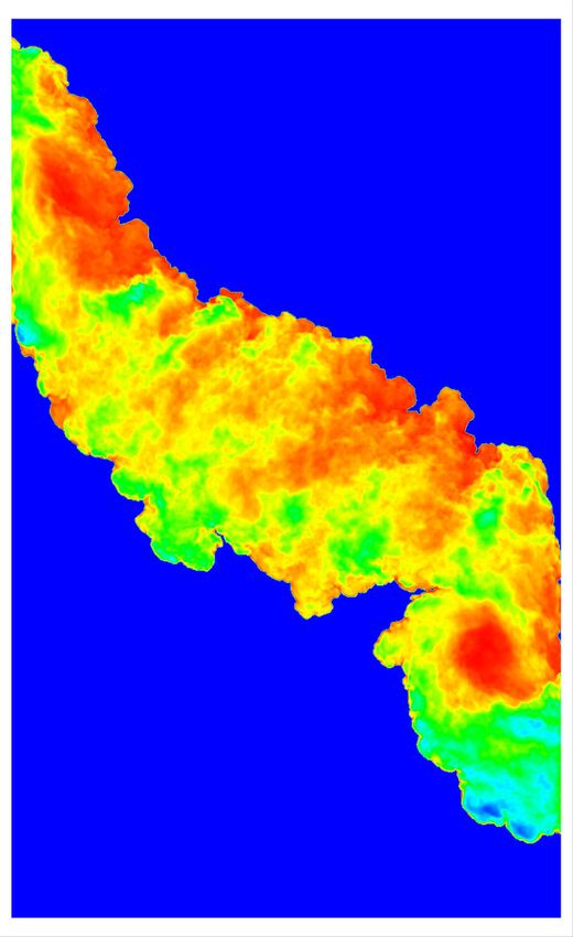
Comparisons of the Favre-averaged mass-fraction (F̃ ) profiles between the models and
iLES at τ =1.741 are shown in Fig. 9. The results at earlier times are very similar. All
19contour plots are normalized by a reference value, and the iso-contour levels shown here are:
0.025, 0.3, 0.7, and 0.975, unless otherwise stated. The K-L and BHR-2 models give the
best results for the overturning spike and bubble plumes. None of the models seem capable
of accurately predicting the bubble plume region due to the excessive isotropic turbulent
diffusion, however, the thickness of the mass-fraction layers across the remainder of the
mixing zone is accurately captured, including the spike plume. In the planar tilted region,
where the mixing is mostly 1D (homogeneous in two directions), the differences between the
models are negligible.
The K profiles are shown in Fig. 10. The K/Kref values predicted by all turbulence
models are consistent with iLES throughout the mixing layer. The BHR-2 model predicts
a width and a shape of the K/Kref iso-contours closer to iLES than the rest of the models.
In the region just above the bubble plume (lower-right “neck”), iLES exhibits a narrow tail-
like feature corresponding to contour level 0.75 (dark grey). Apart from the two-equation
K-L model, all the other models predict a single merged region. The discrepancy is due to
the over-prediction of K, hence turbulent diffusion, at the “neck” by the 3- and 4-equation
models, which causes the two distinct K/Kref =0.75 contour level regions to merge. Since
the “neck” region is highly 2-dimensional, it exemplifies whatever effect the cross-terms
have on the models results, which otherwise vanishes in the 1D simulations. In contrast, in
the region just below the spike plume (upper-left “neck”), all models agree reasonably well
with the iLES solution apart from the K-L; the BHR-2 model provides the most accurate
representation of iLES. Further analysis needs to be carried out in order to draw an accurate
understanding of the models behavior at the highly 2D “neck” regions.
The maximum vertical turbulent mass-flux velocity, max(az ), is accurately predicted by
all models (Fig. 11), with the BHR-2 model showing the closest agreement with the iLES
results at the large-scale bubble and spike plumes. There is some uncertainty regarding the
iLES statistics at late time due to the integral length scale becoming large compare to the
spanwise domain size. This explains the patches of large az /aref
z that can be observed in the
iLES contour plot (Fig. 11d). Whether a larger domain size (Ly >> 15cm) can result in
additional large az contour patches in the tilted mixing region of the 2D averaged iLES and
form a single merged contour level as the BHR-2 model predicts, remains to be investigated.
With regards to the b parameter, each model is found to behave slightly differently but
still provide a reasonable estimate (Fig. 12). The algebraic formulation used in the K-L-a
20model for b is evident by the uniform distribution along the mixing layer. The added-
mass correction factor value used by the K-L-a model is set to c ≈ 2.04 here too, despite
the different fluid partial densities compared to the 1D-RT case. Note that Eq. (20) can
be written in terms of the mass- and volume-fractions only, therefore it is independent of
density. For Atwood numbers other than A ≃ 0.5 as examined here, the value of c would
require adjustment. The K-L-a-b model predicts a narrow band of large b in the tilted region
that can be argued to correspond to the few patches of larger b observed in the iLES. BHR-2
is the only model that correctly predicts the large values of b at the spike and bubble plumes
according to the reference iLES solution.
The BHR-2 model predicts with reasonable accuracy ax , including the area of negative
counter-gradient mass-flux velocity at the top of the tilted mixing layer (Fig. 13). However,
the model is not able to predict the positive flux in the lower half of the tilted mixing region,
where as suggested by Denissen et al. [50], may account for some of the differences in the
mass-fraction contours. Furthermore, the location of the maximum ax value, as well as the
positive value at the front of the spike plume do not agree with the reference iLES solution
either.
The effects of the modified species turbulent diffusion (MSTD) proposed by Bertsch and
Gore [39] are briefly discussed below. MSTD replaces the standard Fickian-like mass-fraction
turbulent transport term by Eq. (27) and can be implemented in conjunction with any tur-
bulence model that includes a transport equation for the turbulent mass-flux velocities (ai ).
Here, the gradient diffusion approximation (GDA) and MSTD assumptions are compared
in the framework of the BHR-2 model, which has given overall the most promising results
this far.
Fig. 14 shows that the MSTD term significantly improves the distribution of F̃ in the
bubble and spike plumes at the expense of a slight increase of the mixing zone width. The
MSTD modification has hardly any effect on the turbulence kinetic energy profiles (plots not
shown here). The SF limiter also offers some improvement to the BHR-2 model, particularly
the large 2D over-turning bubble and spike plume features; however, the best results for the
mass-fraction in the plume regions (with reference to iLES) are obtained by the BHR-2
model with the MSTD approximation.
21V. CONCLUSIONS
This study examined the accuracy of two- to four-equation (linear eddy viscosity) turbu-
lence models for Rayleigh–Taylor induced turbulent mixing through comparisons with high
resolution simulations.
By increasing model complexity in a gradual and systematic manner, a detailed under-
standing of the accuracy and limitations of the models is obtained. Discretization of the
governing and turbulence model equations is kept consistent across all models, thus reducing
accuracy uncertainties associated with the numerical implementation.
The main conclusions drawn from the investigation are summarized below:
• The more complex tilted rig test-case was necessary in order to reveal discrepancies
between the models.
• The K-L-a model [45] provides better accuracy than the K-L model, and also employs
a simpler form of the turbulence kinetic energy production source term. This is evident
by comparing with the production source term, SK , used in Refs. [32, 42].
• The K-L-a-b model presented here is a reduced form of the BHR-2 model. Using a
model transport equation for b provides some accuracy improvement compare to the
algebraic expression used by the K-L-a model, particularly in relation to the prediction
of the turbulent mass-flux velocities and the turbulence kinetic energy results in the
tilted rig test-case.
• In respect of the tilted rig case, the BHR-2 model performs better than K-L-a-b in the
spike but worse in the bubble plume region.
• The turbulent viscosity limiter (SF ) improves the mass-fraction predictions, particu-
larly in the plume regions of the tilted rig case.
• The modified species turbulent diffusion term improved the mass-fraction results, par-
ticularly in the large scale 2D overturning regions of the mixing layer, without adversely
affecting the accuracy of the rest of the results.
• Overall, the BHR-2 model provided the closest results to iLES in the bubble and spike
plume regions.
22Future work is required to address accuracy issues regarding the prediction of (positive)
ax in the lower half of the tilted mixing region, and to further examine the modified species
turbulent diffusion term, as well as the effect of the models cross-terms in highly 2D regions.
ACKNOWLEDGMENTS
Dimitris Drikakis wishes to express his gratitude and appreciation to AWE for their fi-
nancial support through the William Penney Fellowship award. The manuscript contains
material c British Crown Owned Copyright 2018/AWE, reproduced with permission. Re-
sults were obtained using the EPSRC funded ARCHIE-WeSt High Performance Computer
(www.archie-west.ac.uk) under EPSRC Grant No. EP/K000586/1.
[1] P. Amendt, J. D. Colvin, R. E. Tipton, D. E. Hinkel, M. J. Edwards, O. L. Landen, J. D.
Ramshaw, L. J. Suter, W. S. Varnum, and R. G. Watt, Physics of Plasmas 9, 2221 (2002).
[2] V. Smalyuk, O. Hurricane, J. Hansen, G. Langstaff, D. Martinez, H.-S. Park, K. Raman,
B. Remington, H. Robey, O. Schilling, R. Wallace, Y. Elbaz, A. Shimony, D. Shvarts, C. D.
Stefano, R. Drake, D. Marion, C. Krauland, and C. Kuranz, High Energy Density Physics 9,
47 (2013).
[3] J. Decaix and E. Goncalvès, International Journal for Numerical Methods in Fluids 68, 1053
(2012).
[4] J. R. Nanduri, D. R. Parsons, S. L. Yilmaz, I. B. Celik, and P. A. Strakey, Combustion
Science and Technology 182, 794 (2010).
[5] A. S. Almgren, J. B. Bell, C. A. Rendleman, and M. Zingale, The Astrophysical Journal 637,
922 (2006).
[6] W. H. Cabot and A. W. Cook, Nature Physics 2, 562 (2006).
[7] J. M. Pittard, S. A. E. G. Falle, T. W. Hartquist, and J. E. Dyson, Monthly Notices of the
Royal Astronomical Society 394, 1351 (2009).
[8] M. Brüggen, E. Scannapieco, and S. Heinz, Monthly Notices of the Royal Astronomical
Society 395, 2210 (2009).
[9] J. Ferziger, J. Koseff, and S. Monismith, Computers & Fluids 31, 557 (2002).
23[10] F. Grinstein, L. Margolin, and W. Rider, Implicit large eddy simulation: computing turbulent
fluid dynamics (Cambridge Univ Pr, 2007).
[11] D. Drikakis, M. Hahn, A. Mosedale, and B. Thornber, Philosophical Transactions of the Royal
Society of London A: Mathematical, Physical and Engineering Sciences 367, 2985 (2009).
[12] B. Thornber, D. Drikakis, D. Youngs, and R. Williams, Journal of Fluid Mechanics 654, 99
(2010).
[13] M. Lombardini, D. J. Hill, D. I. Pullin, and D. I. Meiron, Journal of Fluid Mechanics 670,
439 (2011).
[14] M. Lombardini, D. I. Pullin, and D. I. Meiron, Journal of Fluid Mechanics 690, 203 (2012).
[15] A. Hadjadj, H. C. Yee, and B. Sjögreen, International Journal for Numerical Methods in
Fluids 70, 1405 (2012).
[16] D. L. Youngs, Philosophical Transactions of the Royal Society A: Mathematical, Physical and
Engineering Sciences 371 (2013), 10.1098/rsta.2012.0173.
[17] F. Grinstein, A. Gowardhan, and J. Ristorcelli, Philosophical Transactions of the Royal
Society A: Mathematical, Physical and Engineering Sciences , 371 (2013).
[18] D. Youngs, Physica Scripta 92 (2017), 10.1088/1402-4896/aa732b.
[19] T. J. Rehagen, J. A. Greenough, and B. J. Olson, Journal of Fluids Engineering 139, 061204
(2017).
[20] B. E. Morgan, B. J. Olson, J. E. White, and J. A. McFarland, Journal of Turbulence 18, 973
(2017).
[21] Y. Zhou, Physics Reports 720-722, 1 (2017).
[22] Y. Zhou, Physics Reports 723-725, 1 (2017).
[23] U. Alon, J. Hecht, D. Ofer, and D. Shvarts, Physical review letters 74, 534 (1995).
[24] J. D. Ramshaw, Physical Review E 58, 5834 (1998).
[25] G. Dimonte and M. Schneider, Physics of Fluids 12, 304 (2000).
[26] B. Cheng, J. Glimm, and D. H. Sharp, Chaos: An Interdisciplinary Journal of Nonlinear
Science 12, 267 (2002).
[27] D. Youngs, Physica D: Nonlinear Phenomena 37, 270 (1989).
[28] D. Youngs, Laser and Particle Beams 12, 725 (1994).
[29] Y. Chen, J. Glimm, D. H. Sharp, and Q. Zhang, Physics of Fluids 8, 816 (1996).
[30] A. Llor, Statistical Hydrodynamic Models for Developing Mixing Instability Flows (Springer,
242005).
[31] S. Gauthier and M. Bonnet, Physics of Fluids A: Fluid Dynamics 2, 1685 (1990).
[32] G. Dimonte and R. Tipton, Physics of Fluids 18, 085101 (2006).
[33] J. T. Morán-López and O. Schilling, High Energy Density Physics 9, 112 (2013).
[34] J. Morán-López and O. Schilling, Shock Waves 24, 325 (2014).
[35] D. Besnard, R. Rauenzahn, and F. Harlow, in Computational Fluid Dynamics; Proceedings
of the International Symposium, Vol. 1, edited by G. de Vahl Davis and C. Fletcher (1988)
pp. 295–304.
[36] A. Banerjee, R. A. Gore, and M. J. Andrews, Physical Review E 82, 046309 (2010).
[37] J. D. Schwarzkopf, D. Livescu, R. A. Gore, R. M. Rauenzahn, and J. R. Ristorcelli, Journal
of Turbulence 12, N49 (2011).
[38] K. Stalsberg-Zarling and R. A. Gore, The bhr2 turbulence model Incompressible isotropic de-
cay, Rayleigh-Taylor, Kelvin-Helmholtz and homogeneous variable density turbulence, Report
LA-UR-11-04773 (LANL, 2011).
[39] R. L. Bertsch and R. A. Gore, RANS simulations of Rayleigh-Taylor Instability Subject to a
changing body force, Report LA-UR-16-24705 (LANL, 2016).
[40] V. Smeeton and D. Youngs, Experimental Investigation of Turbulent Mixing by Rayleigh-
Taylor Instability. Part 3, Report O 35/87 (AWE, 1987).
[41] G. Allaire, S. Clerc, and S. Kokh, Journal of Computational Physics 181, 577 (2002).
[42] I. W. Kokkinakis, D. Drikakis, D. L. Youngs, and R. J. Williams, International Journal of
Heat and Fluid Flow 56, 233 (2015).
[43] F. A. Williams, Combustion Theory (Perseus Books, 1994).
[44] A. W. Cook, Physics of Fluids 21, 055109 (2009).
[45] B. E. Morgan and M. E. Wickett, Phys. Rev. E 91, 043002 (2015).
[46] B. E. Morgan, O. Schilling, and T. A. Hartland, Phys. Rev. E 97, 013104 (2018).
[47] J. D. Schwarzkopf, D. Livescu, J. R. Baltzer, R. A. Gore, and J. R. Ristorcelli, Flow, Turbu-
lence and Combustion 96, 1 (2016).
[48] D. Besnard, F. H. Harlow, R. M. Rauenzahn, and C. Zemach, Turbulence transport equations
for variable-density turbulence and their relationship to two-field models, Report LA-12303-MS
(LANL, 1992).
[49] B. Rollin, N. A. Denissen, J. M. Reisner, and M. J. Andrews, ASME International Mechanical
25Engineering Congress and Exposition Fluids and Heat Transfer, Parts A, B, C, and D, 7, 1353
(2012).
[50] N. A. Denissen, B. Rollin, J. M. Reisner, and M. J. Andrews, Journal of Fluids Engineering
136, 091301 (2014).
[51] B. Vreman, B. Geurts, and H. Kuerten, Journal of Fluid Mechanics 278, 351 (1994).
[52] S. Godunov, Mat. Sb 47, 134 (1959).
[53] K. Kim and C. Kim, Journal of Computational Physics 208, 570 (2005).
[54] B. Thornber, A. Mosedale, D. Drikakis, D. Youngs, and R. Williams, Journal of Computa-
tional Physics 227, 4873 (2008).
[55] E. Toro, M. Spruce, and W. Speares, Shock waves 4, 25 (1994).
[56] D. Drikakis and W. Rider, High-Resolution Methods for Incompressible and Low Speed Flows
(Springer, 2005).
[57] M. Hahn and D. Drikakis, International Journal for Numerical Methods in Fluids 47, 971
(2005).
[58] M. Hahn, D. Drikakis, D. Youngs, and R. Williams, Physics of Fluids 23 (2011),
10.1063/1.3576187.
[59] E. Shapiro and D. Drikakis, Journal of Computational Physics 210, 584 (2005).
[60] D. L. Youngs, Physics of Fluids A: Fluid Dynamics 3, 1312 (1991).
[61] P. Dimotakis, Journal of Fluid Mechanics 409, 69 (2000).
[62] A. Cook and P. Dimotakis, Journal of Fluid Mechanics 443, 69 (2001).
[63] D. Livescu, Philosophical Transactions of the Royal Society A: Mathematical, Physical and
Engineering Sciences 371 (2013), 10.1098/rsta.2012.0185.
[64] D. Livescu, J. R. Ristorcelli, R. A. Gore, S. H. Dean, W. H. Cabot, and A. W. Cook, Journal
of Turbulence 10, 1 (2009).
[65] M. J. Andrews, D. L. Youngs, D. Livescu, and T. Wei, Journal of Fluids Engineering 136,
091212 (2014).
[66] J. M. Holford, S. B. Dalziel, and D. L. Youngs, Laser and Particle Beams 21, 419 (2003).
[67] T. Wei and D. Livescu, in APS Meeting Abstracts (2011).
[68] D. Drikakis, Progress in Aerospace Sciences 39, 405 (2003).
[69] P. Tsoutsanis, I. W. Kokkinakis, L. Könözsy, D. Drikakis, R. J. Williams, and D. L. Youngs,
Computer Methods in Applied Mechanics and Engineering 293, 207 (2015).
26You can also read