ChauffeurNet: Learning to Drive by Imitating the Best and Synthesizing the Worst
←
→
Page content transcription
If your browser does not render page correctly, please read the page content below
ChauffeurNet: Learning to drive by imitating the best and synthesizing the worst

                                                          ChauffeurNet: Learning to Drive
                                                  by Imitating the Best and Synthesizing the Worst

                                        Mayank Bansal                                                               mayban@waymo.com
                                        Waymo Research
                                        Mountain View, CA 94043, USA

                                        Alex Krizhevsky∗                                                       akrizhevsky@gmail.com
arXiv:1812.03079v1 [cs.RO] 7 Dec 2018

                                        Abhijit Ogale                                                                ogale@waymo.com
                                        Waymo Research
                                        Mountain View, CA 94043, USA

                                        Editor:

                                                                                   Abstract
                                            Our goal is to train a policy for autonomous driving via imitation learning that is robust
                                            enough to drive a real vehicle. We find that standard behavior cloning is insufficient
                                            for handling complex driving scenarios, even when we leverage a perception system for
                                            preprocessing the input and a controller for executing the output on the car: 30 million
                                            examples are still not enough. We propose exposing the learner to synthesized data in the
                                            form of perturbations to the expert’s driving, which creates interesting situations such as
                                            collisions and/or going off the road. Rather than purely imitating all data, we augment
                                            the imitation loss with additional losses that penalize undesirable events and encourage
                                            progress – the perturbations then provide an important signal for these losses and lead to
                                            robustness of the learned model. We show that the ChauffeurNet model can handle complex
                                            situations in simulation, and present ablation experiments that emphasize the importance
                                            of each of our proposed changes and show that the model is responding to the appropriate
                                            causal factors. Finally, we demonstrate the model driving a car in the real world.
                                            Keywords: Deep Learning, Mid-to-mid Driving, Learning to Drive, Trajectory Predic-
                                            tion.

                                        1. Introduction
                                        In order to drive a car, a driver needs to see and understand the various objects in the
                                        environment, predict their possible future behaviors and interactions, and then plan how
                                        to control the car in order to safely move closer to their desired destination while obeying
                                        the rules of the road. This is a difficult robotics challenge that humans solve well, making
                                        imitation learning a promising approach. Our work is about getting imitation learning to
                                        the level where it has a shot at driving a real vehicle; although the same insights may apply
                                        to other domains, these domains might have different constraints and opportunities, so we
                                        do not want to claim contributions there.

                                        ∗. Work done while at Google Brain & Waymo.

                                                                                        1
Bansal, Krizhevsky & Ogale
We built our system based on leveraging the training data (30 million real-world expert
driving examples, corresponding to about 60 days of continual driving) as effectively as
possible. There is a lot of excitement for end-to-end learning approaches to driving which
typically focus on learning to directly predict raw control outputs such as steering or braking
after consuming raw sensor input such as camera or lidar data. But to reduce sample
complexity, we opt for mid-level input and output representations that take advantage of
perception and control components. We use a perception system that processes raw sensor
information and produces our input: a top-down representation of the environment and
intended route, where objects such as vehicles are drawn as oriented 2D boxes along with
a rendering of the road information and traffic light states. We present this mid-level input
to a recurrent neural network (RNN), named ChauffeurNet, which then outputs a driving
trajectory that is consumed by a controller which translates it to steering and acceleration.
The further advantage of these mid-level representations is that the net can be trained on
real or simulated data, and can be easily tested and validated in closed-loop simulations
before running on a real car.
Our first finding is that even with 30 million examples, and even with mid-level input and
output representations that remove the burden of perception and control, pure imitation
learning is not sufficient. As an example, we found that this model would get stuck or
collide with another vehicle parked on the side of a narrow street, when a nudging and
passing behavior was viable. The key challenge is that we need to run the system closed-
loop, where errors accumulate and induce a shift from the training distribution (Ross et al.
(2011)). Scientifically, this result is valuable evidence about the limitations of pure imitation
in the driving domain, especially in light of recent promising results for high-capacity models
(Laskey et al. (2017a)). But practically, we needed ways to address this challenge without
exposing demonstrators to new states actively (Ross et al. (2011); Laskey et al. (2017b)) or
performing reinforcement learning (Kuefler et al. (2017)).
We find that this challenge is surmountable if we augment the imitation loss with losses
that discourage bad behavior and encourage progress, and, importantly, augment our data
with synthesized perturbations in the driving trajectory. These expose the model to non-
expert behavior such as collisions and off-road driving, and inform the added losses, teaching
the model to avoid these behaviors. Note that the opportunity to synthesize this data
comes from the mid-level input-output representations, as perturbations would be difficult
to generate with either raw sensor input or direct controller outputs.
We evaluate our system, as well as the relative importance of both loss augmentation
and data augmentation, first in simulation. We then show how our final model successfully
drives a car in the real world and is able to negotiate situations involving other agents, turns,
stop signs, and traffic lights. Finally, it is important to note that there are highly interactive
situations such as merging which may require a significant degree of exploration within a
reinforcement learning (RL) framework. This will demand simulating other (human) traffic
participants, a rich area of ongoing research. Our contribution can be viewed as pushing
the boundaries of what you can do with purely offline data and no RL.
2ChauffeurNet: Learning to drive by imitating the best and synthesizing the worst
2. Related Work
Decades-old work on ALVINN (Pomerleau (1989)) showed how a shallow neural network
could follow the road by directly consuming camera and laser range data. Learning to drive
in an end-to-end manner has seen a resurgence in recent years. Recent work by Chen et al.
(2015) demonstrated a convolutional net to estimate affordances such as distance to the
preceding car that could be used to program a controller to control the car on the highway.
Researchers at NVIDIA (Bojarski et al. (2016, 2017)) showed how to train an end-to-end
deep convolutional neural network that steers a car by consuming camera input. Xu et al.
(2017) trained a neural network for predicting discrete or continuous actions also based
on camera inputs. Codevilla et al. (2018) also train a network using camera inputs and
conditioned on high-level commands to output steering and acceleration. Kuefler et al.
(2017) use Generative Adversarial Imitation Learning (GAIL) with simple affordance-style
features as inputs to overcome cascading errors typically present in behavior cloned policies
so that they are more robust to perturbations. Recent work from Hecker et al. (2018) learns
a driving model using 360-degree camera inputs and desired route planner to predict steering
and speed. The CARLA simulator (Dosovitskiy et al. (2017)) has enabled recent work such
as Sauer et al. (2018), which estimates several affordances from sensor inputs to drive a car
in a simulated urban environment. Using mid-level representations in a spirit similar to our
own, Müller et al. (2018) train a system in simulation using CARLA by training a driving
policy from a scene segmentation network to output high-level control, thereby enabling
transfer learning to the real world using a different segmentation network trained on real
data. Pan et al. (2017) also describes achieving transfer of an agent trained in simulation
to the real world using a learned intermediate scene labeling representation. Reinforcement
learning may also be used in a simulator to train drivers on difficult interactive tasks such
as merging which require a lot of exploration, as shown in Shalev-Shwartz et al. (2016). A
convolutional network operating on a space-time volume of bird’s eye-view representations
is also employed by Luo et al. (2018); Djuric et al. (2018); Lee et al. (2017) for tasks like
3D detection, tracking and motion forecasting. Finally, there exists a large volume of work
on vehicle motion planning outside the machine learning context and Paden et al. (2016)
present a notable survey.
3. Model Architecture
3.1 Input Output Representation
We begin by describing our top-down input representation that the network will process to
output a drivable trajectory. At any time t, our agent (or vehicle) may be represented in
a top-down coordinate system by pt , θt , st , where pt = (xt , yt ) denotes the agent’s location
or pose, θt denotes the heading or orientation, and st denotes the speed. The top-down
coordinate system is picked such that our agent’s pose p0 at the current time t = 0 is
always at a fixed location (u0 , v0 ) within the image. For data augmentation purposes
during training, the orientation of the coordinate system is randomly picked for each training
example to be within an angular range of θ0 ±∆, where θ0 denotes the heading or orientation
of our agent at time t = 0. The top-down view is represented by a set of images of size
W × H pixels, at a ground sampling resolution of φ meters/pixel. Note that as the agent
3Bansal, Krizhevsky & Ogale
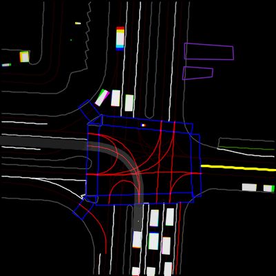
(a) Roadmap (b) Traffic Lights (c) Speed Limit (d) Route
(e) Current Agent (f) Dynamic Boxes (g) Past Agent Poses (h) Future Agent Poses
Box
Figure 1: Driving model inputs (a-g) and output (h).
moves, this view of the environment moves with it so the agent always sees a fixed forward
range, Rf orward = (H − v0 )φ of the world – similar to having an agent with sensors that
see only up to Rf orward meters forward.
As shown in Fig. 1, the input to our model consists of several images of size W × H
pixels rendered into this top-down coordinate system. (a) Roadmap: a color (3-channel)
image with a rendering of various map features such as lanes, stop signs, cross-walks, curbs,
etc. (b) Traffic lights: a temporal sequence of grayscale images where each frame of the
sequence represents the known state of the traffic lights at each past timestep. Within
each frame, we color each lane center by a gray level with the brightest level for red lights,
intermediate gray level for yellow lights, and a darker level for green or unknown lights1 . (c)
Speed limit: a single channel image with lane centers colored in proportion to their known
speed limit. (d) Route: the intended route along which we wish to drive, generated by a
router (think of a Google Maps-style route). (e) Current agent box: this shows our agent’s
full bounding box at the current timestep t = 0. (f) Dynamic objects in the environment:
a temporal sequence of images showing all the potential dynamic objects (vehicles, cyclists,
pedestrians) rendered as oriented boxes. (g) Past agent poses: the past poses of our agent
are rendered into a single grayscale image as a trail of points.
We use a fixed-time sampling of δt to sample any past or future temporal information,
such as the traffic light state or dynamic object states in the above inputs. The traffic
1. We employ an indexed representation for roadmap and traffic lights channels to reduce the number of
input channels, and to allow extensibility of the input representation to express more roadmap features
or more traffic light states without changing the model architecture.
4ChauffeurNet: Learning to drive by imitating the best and synthesizing the worst
(a) Rendered
Inputs
Feature
Net
(b)
Road
Agent Perception
Mask
RNN RNN
Net
Perception
Agent Box Road
Heading Speed Waypoint Box
Heatmap Mask
Heatmap
(c)
Agent On Road
Heading Speed Waypoint Geometry Collision Perception
Box Road Mask
Loss Loss Loss Loss Loss Loss
Loss Loss Loss
Target Target Target Target
Target Target Target
Agent Agent Road Perception
Speed Waypoint Geometry
Heading Box Mask Boxes
Figure 2: Training the driving model. (a) The core ChauffeurNet model with a FeatureNet
and an AgentRNN, (b) Co-trained road mask prediction net and PerceptionRNN, and (c)
Training losses are shown in blue, and the green labels depict the ground-truth data. The
dashed arrows represent the recurrent feedback of predictions from one iteration to the next.
lights and dynamic objects are sampled over the past Tscene seconds, while the past agent
poses are sampled over a potentially longer interval of Tpose seconds. This simple input
representation, particularly the box representation of other dynamic objects, makes it easy
to generate input data from simulation or create it from real-sensor logs using a standard
perception system that detects and tracks objects. This enables testing and validation of
models in closed-loop simulations before running them on a real car. This also allows the
same model to be improved using simulated data to adequately explore rare situations such
as collisions for which real-world data might be difficult to obtain. Using a top-down 2D
view also means efficient convolutional inputs, and allows flexibility to represent metadata
and spatial relationships in a human-readable format. Papers on testing frameworks such
as Tian et al. (2018), Pei et al. (2017) show the brittleness of using raw sensor data (such
as camera images or lidar point clouds) for learning to drive, and reinforce the approach of
using an intermediate input representation.
If I denotes the set of all the inputs enumerated above, then the ChauffeurNet model
recurrently predicts future poses of our agent conditioned on these input images I as shown
by the green dots in Fig. 1(h).
pt+δt = ChauffeurNet(I, pt ) (1)
5Bansal, Krizhevsky & Ogale
M0
add
Memory, M k-1
M1
Past
Agent
Rendered Locations
Inputs
Predicted
Feature k AgentRNN Location, p k M2
Net
Features, F
set
⋮
Predicted
Agent
Box, B k M9
Last
Agent
Box, B k-1
(a) (b)
Figure 3: (a) Schematic of ChauffeurNet. (b) Memory updates over multiple iterations.
In Eq. (1), current pose p0 is a known part of the input, and then the ChauffeurNet
performs N iterations and outputs a future trajectory{pδt , p2δt , ..., pN δt } along with other
properties such as future speeds. This trajectory can be fed to a controls optimizer that
computes detailed driving control (such as steering and braking commands) within the
specific constraints imposed by the dynamics of the vehicle to be driven. Different types of
vehicles may possibly utilize different control outputs to achieve the same driving trajectory,
which argues against training a network to directly output low-level steering and acceleration
control. Note, however, that having intermediate representations like ours does not preclude
end-to-end optimization from sensors to controls.
3.2 Model Design
Broadly, the driving model is composed of several parts as shown in Fig. 2. The main Chauf-
feurNet model shown in part (a) of the figure consists of a convolutional feature network
(FeatureNet) that consumes the input data to create a digested contextual feature repre-
sentation that is shared by the other networks. These features are consumed by a recurrent
agent network (AgentRNN) that iteratively predicts successive points in the driving trajec-
tory. Each point at time t in the trajectory is characterized by its location pt = (xt , yt ),
heading θt and speed st . The AgentRNN also predicts the bounding box of the vehicle as
a spatial heatmap at each future timestep. In part (b) of the figure, we see that two other
networks are co-trained using the same feature representation as an input. The Road Mask
Network predicts the drivable areas of the field of view (on-road vs. off-road), while the
6ChauffeurNet: Learning to drive by imitating the best and synthesizing the worst
New Environment State
Predicted
Data Net Input Neural Waypoints Controls Controls Vehicle Update Environment
Environment Current Pose
Renderer Net Optimization Real/Simulated
Dynamic
Router
New Route
Figure 4: Software architecture for the end-to-end driving pipeline.
recurrent perception network (PerceptionRNN) iteratively predicts a spatial heatmap for
each timestep showing the future location of every other agent in the scene. We believe
that doing well on these additional tasks using the same shared features as the main task
improves generalization on the main task. Fig. 2(c) shows the various losses used in training
the model, which we will discuss in detail below.
Fig. 3 illustrates the ChauffeurNet model in more detail. The rendered inputs shown in
Fig. 1 are fed to a large-receptive field convolutional FeatureNet with skip connections, which
outputs features F that capture the environmental context and the intent. These features
are fed to the AgentRNN which predicts the next point pk on the driving trajectory, and the
agent bounding box heatmap Bk , conditioned on the features F from the FeatureNet, the
iteration number k ∈ {1, . . . , N }, the memory Mk−1 of past predictions from the AgentRNN,
and the agent bounding box heatmap Bk−1 predicted in the previous iteration.
pk , Bk = AgentRNN(k, F, Mk−1 , Bk−1 ) (2)
The memory Mk is an additive memory consisting of a single channel image. At iteration
k of the AgentRNN, the memory is incremented by 1 at the location pk predicted by the
AgentRNN, and this memory is then fed to the next iteration. The AgentRNN outputs a
heatmap image over the next pose of the agent, and we use the arg-max operation to obtain
the coarse pose prediction pk from this heatmap. The AgentRNN then employs a shallow
convolutional meta-prediction network with a fully-connected layer that predicts a sub-pixel
refinement of the pose δpk and also estimates the heading θk and the speed sk . Note that
the AgentRNN is unrolled at training time for a fixed number of iterations, and the losses
described below are summed together over the unrolled iterations. This is possible because
of the non-traditional RNN design where we employ an explicitly crafted memory model
instead of a learned memory.
3.3 System Architecture
Fig. 4 shows a system level overview of how the neural net is used within the self-driving
system. At each time, the updated state of our agent and the environment is obtained via
a perception system that processes sensory output from the real-world or from a simulation
environment as the case may be. The intended route is obtained from the router, and is
updated dynamically conditioned on whether our agent was able to execute past intents or
not. The environment information is rendered into the input images described in Fig. 1
and given to the RNN which then outputs a future trajectory. This is fed to a controls
optimizer that outputs the low-level control signals that drive the vehicle (in the real world
or in simulation).
7Bansal, Krizhevsky & Ogale
4. Imitating the Expert
In this section, we first show how to train the model above to imitate the expert.
4.1 Imitation Losses
4.1.1 Agent Position, Heading and Box Prediction
The AgentRNN produces three outputs at each iteration k: a probability distribution
Pk (x, y) over the spatial coordinates of the predicted waypoint obtained after a spatial
softmax, a heatmap of the predicted agent box at that timestep Bk (x, y) obtained after a
per-pixel sigmoid activation that represents the probability that the agent occupies a par-
ticular pixel, and a regressed box heading output θk . Given ground-truth data for the above
predicted quantities, we can define the corresponding losses for each iteration as:
Lp = H(Pk , Pkgt ) (3)
1 XX
LB = H(Bk (x, y), Bkgt (x, y)) (4)
WH x y
Lθ = θk − θkgt (5)
1
where the superscript gt denotes the corresponding ground-truth values, and H(a, b) is the
cross-entropy function. Note that Pkgt is a binary image with only the pixel at the ground-
truth target coordinate bpgt
k c set to one.
4.1.2 Agent Meta Prediction
The meta prediction network performs regression on the features to generate a sub-pixel
refinement δpk of the coarse waypoint prediction as well as a speed estimate sk at each
iteration. We employ L1 loss for both of these outputs:
Lp−subpixel = δpk − δpgt
k (6)
1
Lspeed = sk − sgt
k (7)
1
where δpgt gt gt
k = pk − bpk c is the fractional part of the ground-truth pose coordinates.
4.2 Past Motion Dropout
During training, the model is provided the past motion history as one of the inputs (Fig. 1(g)).
Since the past motion history during training is from an expert demonstration, the net can
learn to “cheat” by just extrapolating from the past rather than finding the underlying
causes of the behavior. During closed-loop inference, this breaks down because the past
history is from the net’s own past predictions. For example, such a trained net may learn to
only stop for a stop sign if it sees a deceleration in the past history, and will therefore never
stop for a stop sign during closed-loop inference. To address this, we introduce a dropout
on the past pose history, where for 50% of the examples, we keep only the current position
(u0 , v0 ) of the agent in the past agent poses channel of the input data. This forces the net
8ChauffeurNet: Learning to drive by imitating the best and synthesizing the worst
(a) Original (b) Perturbed
Figure 5: Trajectory Perturbation. (a) An original logged training example where the agent
is driving along the center of the lane. (b) The perturbed example created by perturbing
the current agent location (red point) in the original example away from the lane center
and then fitting a new smooth trajectory that brings the agent back to the original target
location along the lane center.
to look at other cues in the environment to explain the future motion profile in the training
example.
5. Beyond Pure Imitation
In this section, we go beyond vanilla cloning of the expert’s demonstrations in order to teach
the model to arrest drift and avoid bad behavior such as collisions and off-road driving by
synthesizing variations of the expert’s behavior.
5.1 Synthesizing Perturbations
Running the model as a part of a closed-loop system over time can cause the input data
to deviate from the training distribution. To prevent this, we train the model by adding
some examples with realistic perturbations to the agent trajectories. The start and end of
a trajectory are kept constant, while a perturbation is applied around the midpoint and
smoothed across the other points. Quantitatively, we jitter the midpoint pose of the agent
uniformly at random in the range [−0.5, 0.5] meters in both axes, and perturb the heading
by [−π/3, π/3] radians. We then fit a smooth trajectory to the perturbed point and the
original start and end points. Such training examples bring the car back to its original
trajectory after a perturbation. Fig. 5 shows an example of perturbing the current agent
location (red point) away from the lane center and the fitted trajectory correctly bringing
it back to the original target location along the lane center. We filter out some perturbed
trajectories that are impractical by thresholding on maximum curvature. But we do allow
the perturbed trajectories to collide with other agents or drive off-road, because the network
can then experience and avoid such behaviors even though real examples of these cases are
9Bansal, Krizhevsky & Ogale
not present in the training data. In training, we give perturbed examples a weight of 1/10
relative to the real examples, to avoid learning a propensity for perturbed driving.
5.2 Beyond the Imitation Loss
5.2.1 Collision Loss
Since our training data does not have any real collisions, the idea of avoiding collisions is
implicit and will not generalize well. To alleviate this issue, we add a specialized loss that
directly measures the overlap of the predicted agent box Bk with the ground-truth boxes
of all the scene objects at each timestep.
1 XX
Lcollision = Bk (x, y) . Objkgt (x, y) (8)
WH x y
where Bk is the likelihood map for the output agent box prediction, and Objkgt is a binary
mask with ones at all pixels occupied by other dynamic objects (other vehicles, pedestrians,
etc.) in the scene at timestep k. At any time during training, if the model makes a
poor prediction that leads to a collision, the overlap loss would influence the gradients to
correct the mistake. However, this loss would be effective only during the initial training
rounds when the model hasn’t learned to predict close to the ground-truth locations due
to the absence of real collisions in the ground truth data. This issue is alleviated by the
addition of trajectory perturbation data, where artificial collisions within those examples
allow this loss to be effective throughout training without the need for online exploration
like in reinforcement learning settings.
5.2.2 On Road Loss
Trajectory perturbations also create synthetic cases where the car veers off the road or
climbs a curb or median because of the perturbation. To train the network to avoid hitting
such hard road edges, we add a specialized loss that measures overlap of the predicted agent
box Bk in each timestep with a binary mask Roadgt denoting the road and non-road regions
within the field-of-view.
1 XX
Lonroad = Bk (x, y) . (1 − Roadgt (x, y)) (9)
WH x y
5.2.3 Geometry Loss
We would like to explicitly constrain the agent to follow the target geometry independent
of the speed profile. We model this target geometry by fitting a smooth curve to the target
waypoints and rendering this curve as a binary image in the top-down coordinate system.
The thickness of this curve is set to be equal to the width of the agent. We express this
loss similar to the collision loss by measuring the overlap of the predicted agent box with
the binary target geometry image Geomgt . Any portion of the box that does not overlap
with the target geometry curve is added as a penalty to the loss function.
1 XX
Lgeom = Bk (x, y) . (1 − Geomgt (x, y)) (10)
WH x y
10ChauffeurNet: Learning to drive by imitating the best and synthesizing the worst
(a) Flattened Inputs (b) Target Road Mask (c) Pred Road Mask (d) Pred Vehicles Logits
Logits
(e) Agent Pose Logits (f) Collision Loss (g) On Road Loss (h) Geometry Loss
Figure 6: Visualization of predictions and loss functions on an example input. The top row
is at the input resolution, while the bottom row shows a zoomed-in view around the current
agent location.
5.2.4 Auxiliary Losses
Similar to our own agent’s trajectory, the motion of other agents may also be predicted
by a recurrent network. Correspondingly, we add a recurrent perception network Percep-
tionRNN that uses as input the shared features F created by the FeatureNet and its own
predictions Objk−1 from the previous iteration, and predicts a heatmap Objk at each it-
eration. Objk (x, y) denotes the probability that location (x, y) is occupied by a dynamic
object at time k. For iteration k = 0, the PerceptionRNN is fed the ground truth objects
at the current time.
1 XX
Lobjects = H(Objk (x, y), Objkgt (x, y)) (11)
WH x y
Co-training a PerceptionRNN to predict the future of other agents by sharing the same
feature representation F used by the PerceptionRNN is likely to induce the feature net-
work to learn better features that are suited to both tasks. Several examples of predicted
trajectories from PerceptionRNN on logged data are shown on our website here.
We also co-train to predict a binary road/non-road mask by adding a small network of
convolutional layers to the output of the feature net F . We add a cross-entropy loss to the
predicted road mask output Road(x, y) which compares it to the ground-truth road mask
11Bansal, Krizhevsky & Ogale
Tscene Tpose δt N ∆ W H u0 v0 φ
1.0 s 8.0 s 0.2s 10 25◦ 400 px 400 px 200 px 320 px 0.2 m/px
Table 1: Parameter values for the experiments in this paper.
Rendering FeatureNet AgentRNN (N=10) PerceptionRNN (N=10) Overall
8 ms 6.5 ms 145 ms 35 ms 160 ms
Table 2: Run-time performance on NVIDIA Tesla P100 GPU.
Roadgt .
1 XX
Lroad = H(Road(x, y), Roadgt (x, y)) (12)
WH x y
Fig. 6 shows some of the predictions and losses for a single example processed through
the model.
5.3 Imitation Dropout
Overall, our losses may be grouped into two sub-groups, the imitation losses:
Limit = {Lp , LB , Lθ , Lp−subpixel , Lspeed } (13)
and the environment losses:
Lenv = {Lcollision , Lonroad , Lgeom , Lobjects , Lroad } (14)
The imitation losses cause the model to imitate the expert’s demonstrations, while the
environment losses discourage undesirable behavior such as collisions. To further increase
the effectiveness of the environment losses, we experimented with randomly dropping out
the imitation losses for a random subset of training examples. We refer to this as “imitation
dropout”. In the experiments, we show that imitation dropout yields a better driving model
than simply under-weighting the imitation losses. During imitation dropout, the weight on
the imitation losses wimit is randomly chosen to be either 0 or 1 with a certain probability
for each training example. The overall loss is given by:
X X
L = wimit ` + wenv ` (15)
`∈Limit `∈Lenv
6. Experiments
6.1 Data
The training data to train our model was obtained by randomly sampling segments of real-
world expert driving and removing segments where the car was stationary for long periods
of time. Our input field of view is 80m × 80m (W φ = 80) and with the agent positioned
at (u0 , v0 ), we get an effective forward sensing range of Rf orward = 64m. Therefore, for the
12ChauffeurNet: Learning to drive by imitating the best and synthesizing the worst
experiments in this work we also removed any segments of highway driving given the longer
sensing range requirement that entails. Our dataset contains approximately 26 million
examples which amount to about 60 days of continuous driving. As discussed in Section 3,
the vertical-axis of the top-down coordinate system for each training example is randomly
oriented within a range of ∆ = ±25◦ of our agent’s current heading, in order to avoid a bias
for driving along the vertical axis. The rendering orientation is set to the agent heading
(∆ = 0) during inference. Data about the prior map of the environment (roadmap) and the
speed-limits along the lanes is collected apriori. For the dynamic scene entities like objects
and traffic-lights, we employ a separate perception system based on laser and camera data
similar to existing works in the literature (Yang et al. (2018); Fairfield and Urmson (2011)).
Table 1 lists the parameter values used for all the experiments in this paper. The model
runs on a NVidia Tesla P100 GPU in 160ms with the detailed breakdown in Table 2.
6.2 Models
We train and test not only our final model, but a sequence of models that introduce the
ingredients we describe one by one on top of behavior cloning. We start with M0 , which
does behavior cloning with past motion dropout to prevent using the history to cheat.
M1 adds perturbations without modifying the losses. M2 further adds our environment
losses Lenv in Section 5.2. M3 and M4 address the fact that we do not want to imitate
bad behavior – M3 is a baseline approach, where we simply decrease the weight on the
imitation loss, while M4 uses our imitation dropout approach with a dropout probability
of 0.5. Table 3 lists the configuration for each of these models.
6.3 Closed Loop Evaluation
To evaluate our learned model on a specific scenario, we replay the segment through the
simulation until a buffer period of max(Tpose , Tscene ) has passed. This allows us to generate
the first rendered snapshot of the model input using all the replayed messages until now.
The model is evaluated on this input, and the fitted controls are passed to the vehicle
simulator that emulates the dynamics of the vehicle thus moving the simulated agent to its
next pose. At this point, the simulated pose might be different from the logged pose, but
our input representation allows us to correctly render the new input for the model relative
to the new pose. This process is repeated until the end of the segment, and we evaluate
scenario specific metrics like stopping for a stop-sign, collision with another vehicle etc.
during the simulation. Since the model is being used to drive the agent forward, this is a
closed-loop evaluation setup.
6.3.1 Model Ablation Tests
Here, we present results from experiments using the various models in the closed-loop
simulation setup. We first evaluated all the models on simple situations such as stopping
for stop-signs and red traffic lights, and lane following along straight and curved roads by
creating 20 scenarios for each situation, and found that all the models worked well in these
simple cases. Therefore, we will focus below on specific complex situations that highlight
the differences between these models.
13Bansal, Krizhevsky & Ogale
Model Description wimit wenv
M0 Imitation with Past Dropout 1.0 0.0
M1 M0 + Traj Perturbation 1.0 0.0
M2 M1 + Environment Losses 1.0 1.0
M3 M2 with less imitation 0.5 1.0
M4 M2 with Imitation Dropout Dropout probability = 0.5 (see Section 5.3).
Table 3: Model configuration for the model ablation tests.
Nudging 0% 0% 0% 0%
10%
for a 20% 30%
Passes 40%
55% 45% 60% 55% 45%
Parked Collides
50% 90%
Gets Stuck
Car [video]
0% 0% 0%
Trajectory
Perturba- Recovers 50% 50% 50% 50%
Gets Stuck
tion [video] 100% 100% 100%
0% 0% 0%
5% 5%
Slowing for 10%
5%
25%
a Slow Car Slows Down 0%
Collides 75%
[video] Gets Stuck 95% 95% 100% 85%
M0 M1 M2 M3 M4
Figure 7: Model ablation test results on three scenario types.
Nudging around a parked car. To set up this scenario, we place the agent at an
arbitrary distance from a stop-sign on an undivided two-way street and then place a parked
vehicle on the right shoulder between the the agent and the stop-sign. We pick 4 separate
locations with both straight and curved roads then vary the starting speed of the agent
between 5 different values to create a total of 20 scenarios. We then observe if the agent
would stop and get stuck behind, collide with the parked car, or correctly pass around the
parked car, and report the aggregate performance in Fig. 7(row 1). We find that other than
M4 , all other models cause the agent to collide with the parked vehicle about half the time.
The baseline M0 model can also get stuck behind the parked vehicle in some of the scenarios.
The model M4 nudges around the parked vehicle and then brings the agent back to the
lane center. This can be attributed to the model’s ability to learn to avoid collisions and
nudge around objects because of training with the collision loss the trajectory perturbation.
Comparing model M3 and M4 , it is apparent that “imitation dropout” was more effective
at learning the right behavior than only re-weighting the imitation losses. Note that in
this scenario, we generate several variations by changing the starting speed of the agent
relative to the parked car. This creates situations of increasing difficulty, where the agent
approaches the parked car at very high relative speed and thus does not have enough time
to nudge around the car given the dynamic constraints. A 10% collision rate for M4 is
thus not a measure of the absolute performance of the model since we do not have a perfect
14ChauffeurNet: Learning to drive by imitating the best and synthesizing the worst
driver which could have performed well at all the scenarios here. But in relative terms, this
model performs the best.
Recovering from a trajectory perturbation. To set up this scenario, we place the
agent approaching a curved road and vary the starting position and the starting speed of
the agent to generate a total of 20 scenario variations. Each variation puts the agent at
a different amount of offset from the lane center with a different heading error relative to
the lane. We then measure how well the various models are at recovering from the lane
departure. Fig. 7(row 2) presents the results aggregated across these scenarios and shows
the contrast between the baseline model M0 which is not able to recover in any of the
situations and the models M3 and M4 which handle all deviations well. All models trained
with the perturbation data are able to handle 50% of the scenarios which have a lower
starting speed. At a higher starting speed, we believe that M3 and M4 do better than M1
and M2 because they place a higher emphasis on the imagination losses.
Slowing down for a slow car. To set up this scenario, we place the agent on a straight
road at varying initial speeds and place another car ahead with a varying but slower constant
speed, generating a total of 20 scenario variations, to evaluate the ability to slow for and
then follow the car ahead. From Fig. 7(row 3), we see that some models slow down to zero
speed and get stuck. For the variation with the largest relative speed, there isn’t enough
time for most models to stop the agent in time, thus leading to a collision. For these cases,
model M3 which uses imitation loss re-weighting works better than the model M4 which
uses imitation dropout. M4 has trouble in two situations due to being over aggressive in
trying to maneuver around the slow car and then grazes the left edge of the road. This
happens in the two extreme variations where the relative speed between the two cars is the
highest.
6.3.2 Input Ablation Tests
With input ablation tests, we want to test the final M4 model’s ability to identify the correct
causal factors behind specific behaviors, by testing the model’s behavior in the presence or
absence of the correct causal factor while holding other conditions constant. In simulation,
we have evaluated our model on 20 scenarios with and without stop-signs rendered, and
20 scenarios with and without other vehicles in the scene rendered. The model exhibits
the correct behavior in all scenarios, thus confirming that it has learned to respond to the
correct features for a stop-sign and a stopped vehicle.
6.3.3 Logged Data Simulated Driving
For this evaluation, we take logs from our real-driving test data (separate from our training
data), and use our trained network to drive the car using the vehicle simulator keeping
everything else the same i.e. the dynamic objects, traffic-light states etc. are all kept the
same as in the logs. Some example videos are shown here and they illustrate the ability of
the model in dealing with multiple dynamic objects and road controls.
15Bansal, Krizhevsky & Ogale
Mean L2 distance error M0 M4 M0 M1
Mean L2 distance error
4 4
(pixels)
(pixels)
2 2
0 0
w0 w1 w2 w3 w4 w5 w6 w7 w8 w9 w0 w1 w2 w3 w4 w5 w6 w7 w8 w9
Waypoint Waypoint
(a) Prediction Error for models M0 and M4 on (b) Prediction Error for models M0 and M1 on
unperturbed evaluation data. perturbed evaluation data.
Figure 8: Open loop evaluation results.
6.3.4 Real World Driving
We have also evaluated this model on our self-driving car by replacing the existing planner
module with the learned model M4 and have replicated the driving behaviors observed in
simulation. The videos of several of these runs are available here and they illustrate not only
the smoothness of the network’s driving ability, but also its ability to deal with stop-signs
and turns and to drive for long durations in full closed-loop control without deviating from
the trajectory.
6.4 Open Loop Evaluation
In an open-loop evaluation, we take test examples of expert driving data and for each
example, compute the L2 distance error between the predicted and ground-truth waypoints.
Unlike the closed-loop setting, the predictions are not used to drive the agent forward and
thus the network never sees its own predictions as input. Fig. 8a shows the L2 distance
metric in this open-loop evaluation setting for models M0 and M4 on a test set of 10,000
examples. These results show that model M0 makes fewer errors than the full model M4 ,
but we know from closed-loop testing that M4 is a far better driver than M0 . This shows
how open-loop evaluations can be misleading, and closed-loop evaluations are critical while
assessing the real performance of such driving models.
We also compare the performance of models M0 and M1 on our perturbed evaluation
data w.r.t the L2 distance metric in Fig. 8b. Note that the model trained without including
perturbed data (M0 ) has larger errors due to its inability to bring the agent back from the
perturbation onto its original trajectory. Fig. 9 shows examples of the trajectories predicted
by these models on a few representative examples showcasing that the perturbed data is
critical to avoiding the veering-off tendency of the model trained without such data.
6.5 Failure Modes
At our ground resolution of 20 cm/pixel, the agent currently sees 64 m in front and 40
m on the sides and this limits the model’s ability to perform merges on T-junctions and
16ChauffeurNet: Learning to drive by imitating the best and synthesizing the worst
(a) Ground-truth (b) Model M0 Prediction (c) Model M1 Prediction
Figure 9: Comparison of ground-truth trajectory in (a) with the predicted trajectories from
models M0 and M1 in (b) and (c) respectively on two perturbed examples. The red point
is the reference pose (u0 , v0 ), white points are the past poses and green points are the future
poses.
turns from a high-speed road. Specific situations like U-turns and cul-de-sacs are also not
currently handled, and will require sampling enough training data. The model occasionally
gets stuck in some low speed nudging situations. It sometimes outputs turn geometries that
make the specific turn infeasible (e.g. large turning radius). We also see some cases where
the model gets over aggressive in novel and rare situations for example by trying to pass
a slow moving vehicle. We believe that adequate simulated exploration may be needed for
highly interactive or rare situations.
6.6 Sampling Speed Profiles
The waypoint prediction from the model at timestep k is represented by the probability
distribution Pk (x, y) over the spatial domain in the top-down coordinate system. In this
paper, we pick the mode of this distribution pk to update the memory of the AgentRN N .
More generally, we can also sample from this distribution to allow us to predict trajectories
with different speed profiles. Fig. 10 illustrates the predictions P1 (x, y) and P5 (x, y) at
the first and the fifth iterations respectively, for a training example where the past motion
history has been dropped out. Correspondingly, P1 (x, y) has a high uncertainity along the
longitudinal position and allows us to pick from a range of speed samples. Once we pick
a specific sample, the ensuing waypoints get constrained in their ability to pick different
speeds and this shows as a centered distribution at the P5 (x, y).
17Bansal, Krizhevsky & Ogale
(a) log P1 (x, y) (b) log P5 (x, y)
Figure 10: Sampling speed profiles. The probability distribution P1 (x, y) predicted by the
model at timestep k = 1 allows us to sample different speed profiles conditioned on which
the later distribution P5 (x, y) gets more constrained.
The use of a probability distribution over the next waypoint also presents the inter-
esting possibility of constraining the model predictions at inference time to respect hard
constraints. For example, such constrained sampling may provide a way to ensure that any
trajectories we generate strictly obey legal restrictions such as speed limits. One could also
constrain sampling of trajectories to a designated region, such as a region around a given
reference trajectory.
7. Discussion
In this paper, we presented our experience with what it took to get imitation learning
to perform well in real-world driving. We found that key to its success is synthesizing
interesting situations around the expert’s behavior and augmenting appropriate losses that
discourage undesirable behavior. This constrained exploration is what allowed us to avoid
collisions and off-road driving even though such examples were not explicitly present in
the expert’s demonstrations. To support it, and to best leverage the expert data, we used
middle-level input and output representations which allow easy mixing of real and simulated
data and alleviate the burdens of learning perception and control. With these ingredients,
we got a model good enough to drive a real car. That said, the model is not yet fully
competitive with motion planning approaches but we feel that this is a good step forward
for machine learned driving models. There is room for improvement: comparing to end-to-
end approaches, and investigating alternatives to imitation dropout are among them. But
most importantly, we believe that augmenting the expert demonstrations with a thorough
exploration of rare and difficult scenarios in simulation, perhaps within a reinforcement
learning framework, will be the key to improving the performance of these models especially
for highly interactive scenarios.
Acknowledgments
We would like to thank Andrew Barton-Sweeney for help running the model on the car,
Aleksandar Gabrovski for help with the simulation, Anca Dragan and Dragomir Anguelov
for reviewing the paper and suggesting several improvements.
18ChauffeurNet: Learning to drive by imitating the best and synthesizing the worst
References
Mariusz Bojarski, Davide Del Testa, Daniel Dworakowski, Bernhard Firner, Beat Flepp,
Prasoon Goyal, Lawrence D Jackel, Mathew Monfort, Urs Muller, Jiakai Zhang, et al.
End to end learning for self-driving cars. arXiv preprint arXiv:1604.07316, 2016.
Mariusz Bojarski, Philip Yeres, Anna Choromanska, Krzysztof Choromanski, Bernhard
Firner, Lawrence Jackel, and Urs Muller. Explaining how a deep neural network trained
with end-to-end learning steers a car. arXiv preprint arXiv:1704.07911, 2017.
Chenyi Chen, Ari Seff, Alain Kornhauser, and Jianxiong Xiao. Deepdriving: Learning
affordance for direct perception in autonomous driving. In Proceedings of the IEEE
International Conference on Computer Vision, pages 2722–2730, 2015.
Felipe Codevilla, Matthias Müller, Antonio López, Vladlen Koltun, and Alexey Dosovit-
skiy. End-to-end driving via conditional imitation learning. In 2018 IEEE International
Conference on Robotics and Automation (ICRA), pages 1–9. IEEE, 2018.
Nemanja Djuric, Vladan Radosavljevic, Henggang Cui, Thi Nguyen, Fang-Chieh Chou,
Tsung-Han Lin, and Jeff Schneider. Motion prediction of traffic actors for autonomous
driving using deep convolutional networks. arXiv preprint arXiv:1808.05819, 2018.
Alexey Dosovitskiy, German Ros, Felipe Codevilla, Antonio Lopez, and Vladlen Koltun.
Carla: An open urban driving simulator. arXiv preprint arXiv:1711.03938, 2017.
Nathaniel Fairfield and Chris Urmson. Traffic light mapping and detection. In Robotics and
Automation (ICRA), 2011 IEEE International Conference on, pages 5421–5426. IEEE,
2011.
Simon Hecker, Dengxin Dai, and Luc Van Gool. Learning driving models with a surround-
view camera system and a route planner. arXiv preprint arXiv:1803.10158, 2018.
Alex Kuefler, Jeremy Morton, Tim Wheeler, and Mykel Kochenderfer. Imitating driver
behavior with generative adversarial networks. In Intelligent Vehicles Symposium (IV),
2017 IEEE, pages 204–211. IEEE, 2017.
Michael Laskey, Caleb Chuck, Jonathan Lee, Jeffrey Mahler, Sanjay Krishnan, Kevin
Jamieson, Anca Dragan, and Ken Goldberg. Comparing human-centric and robot-centric
sampling for robot deep learning from demonstrations. In Robotics and Automation
(ICRA), 2017 IEEE International Conference on, pages 358–365. IEEE, 2017a.
Michael Laskey, Jonathan Lee, Roy Fox, Anca Dragan, and Ken Goldberg. Dart: Noise
injection for robust imitation learning. arXiv preprint arXiv:1703.09327, 2017b.
Donghan Lee, Youngwook Paul Kwon, Sara McMains, and J Karl Hedrick. Convolution
neural network-based lane change intention prediction of surrounding vehicles for acc.
In Intelligent Transportation Systems (ITSC), 2017 IEEE 20th International Conference
on, pages 1–6. IEEE, 2017.
19Bansal, Krizhevsky & Ogale
Wenjie Luo, Bin Yang, and Raquel Urtasun. Fast and furious: Real time end-to-end 3d
detection, tracking and motion forecasting with a single convolutional net. In Proceedings
of the IEEE Conference on Computer Vision and Pattern Recognition. IEEE, 2018.
Matthias Müller, Alexey Dosovitskiy, Bernard Ghanem, and Vladen Koltun. Driving policy
transfer via modularity and abstraction. arXiv preprint arXiv:1804.09364, 2018.
Brian Paden, Michal Čáp, Sze Zheng Yong, Dmitry Yershov, and Emilio Frazzoli. A survey
of motion planning and control techniques for self-driving urban vehicles. IEEE Trans-
actions on intelligent vehicles, 1(1):33–55, 2016.
Xinlei Pan, Yurong You, Ziyan Wang, and Cewu Lu. Virtual to real reinforcement learning
for autonomous driving. arXiv preprint arXiv:1704.03952, 2017.
Kexin Pei, Yinzhi Cao, Junfeng Yang, and Suman Jana. Deepxplore: Automated whitebox
testing of deep learning systems. In Proceedings of the 26th Symposium on Operating
Systems Principles, pages 1–18. ACM, 2017.
Dean A Pomerleau. Alvinn: An autonomous land vehicle in a neural network. In Advances
in neural information processing systems, pages 305–313, 1989.
Stéphane Ross, Geoffrey Gordon, and Drew Bagnell. A reduction of imitation learning
and structured prediction to no-regret online learning. In Proceedings of the fourteenth
international conference on artificial intelligence and statistics, pages 627–635, 2011.
Axel Sauer, Nikolay Savinov, and Andreas Geiger. Conditional affordance learning for
driving in urban environments. arXiv preprint arXiv:1806.06498, 2018.
Shai Shalev-Shwartz, Shaked Shammah, and Amnon Shashua. Safe, multi-agent, reinforce-
ment learning for autonomous driving. arXiv preprint arXiv:1610.03295, 2016.
Yuchi Tian, Kexin Pei, Suman Jana, and Baishakhi Ray. Deeptest: Automated testing of
deep-neural-network-driven autonomous cars. In Proceedings of the 40th International
Conference on Software Engineering, pages 303–314. ACM, 2018.
Huazhe Xu, Yang Gao, Fisher Yu, and Trevor Darrell. End-to-end learning of driving models
from large-scale video datasets. In Proceedings of the IEEE Conference on Computer
Vision and Pattern Recognition, pages 2174–2182, 2017.
Bin Yang, Ming Liang, and Raquel Urtasun. Hdnet: Exploiting hd maps for 3d object
detection. In Conference on Robot Learning, pages 146–155, 2018.
20You can also read