Currency Risk Management: Predicting the EUR/ USD Exchange Rate - Digital WPI
←
→
Page content transcription
If your browser does not render page correctly, please read the page content below
Worcester Polytechnic Institute
Digital WPI
Major Qualifying Projects (All Years)                                                                                  Major Qualifying Projects

April 2018

Currency Risk Management: Predicting the EUR/
USD Exchange Rate
Andrea C. Bayas
Worcester Polytechnic Institute

Follow this and additional works at: https://digitalcommons.wpi.edu/mqp-all

Repository Citation
Bayas, A. C. (2018). Currency Risk Management: Predicting the EUR/USD Exchange Rate. Retrieved from
https://digitalcommons.wpi.edu/mqp-all/3661

This Unrestricted is brought to you for free and open access by the Major Qualifying Projects at Digital WPI. It has been accepted for inclusion in
Major Qualifying Projects (All Years) by an authorized administrator of Digital WPI. For more information, please contact digitalwpi@wpi.edu.
Worcester Polytechnic Institute
     Zurich School of Applied Sciences (ZHAW)

            Currency Risk Management
Predicting the EUR/USD Exchange Rate

                                                  Advisor:
  Author:
                                        Dr. Gu Wang, WPI
  Andrea Bayas
                               Dr. Joerg Oesterrider, ZHAW

                    April 26, 2018
1 Abstract
This project provides a simple, yet comprehensive approach to predicting movements in the
exchange rate between the Euro and the U.S. Dollar through the development of a linear regression
model and further fitting the errors by using momentum signals. The predictions generated are
compared to the forward rates in order to develop a hedging strategy for deciding when to use a
forward contract or wait to use the spot exchange rate. Finally, we analyze the payoffs obtained
by using this strategy.
12 Executive Summary
This Major Qualifying Project aims to understand some of the hedging techniques used in the
foreign exchange market, and to develop a simple model to predict the exchange rate between the
Euro (EUR) and the US Dollar (USD), i.e. the EUR/USD exchange rate. The prediction results
are used to help investors hedge against short term exchange rate risk, and tested empirically.
There are three main investment strategies used by currency traders in the Foreign Exchange
market, which is also known as FX and Forex. One is Carry, which prioritizes buying currencies that
pay high interest rates and selling currencies with low interest rates in order to obtain the difference
between interest rates as the payoff. The second strategy is called Valuation, and rises from the
long-run currency tendencies to reach their “fair value”. Thus, traders buy undervalued currencies
since their price is expected to go up, and sell overvalued currencies. Finally, Momentum is a
strategy that arises from a common characteristic observed in the Forex market in which exchange
rates tend to maintain a positive or negative trend for a relatively long period of time. Therefore,
traders buy currencies that have been performing well while selling badly performing currencies.
Based on the theories behind these investment strategies, a linear regression model to predict
the EUR/USD exchange rate was built by choosing the Purchasing Power Parity (PPP), which
represents Valuation, Basis SWAP Libor rates, which represents Carry, and historical volatility,
as the risk measure, to be the predictor variables. We then incorporate a Momentum signal from
the difference of two EWMA’s to improve the accuracy of our predictions by using another linear
regression model to fit the error obtained in our previous model.
To confirm the effectiveness of our predictions we generate a trading strategy to decide whether
we should wait until next month to make the transaction or enter a forward contract based on the
comparison between the predictions and the corresponding forward rates. We obtain the payoff
given by always entering the forward contract, choosing to enter according to our first model, and
choosing to enter according to our improved model. We find that in both latter cases we generate
a positive profit, confirming the effectiveness of this approach to predict the EUR/USD exchange
rates.
23 Acknowledgements
I would like to thank the following individuals and organization for their contributions and support
towards the success of this project.
My advisor, Professor Gu Wang, for his advice, availability and support throughout the course of
this project.
Dr. Joerg Osterrieder, my advisor in ZHAW, for orchestrating meetings with experts in the fields
and encouraging me during my time in Switzerland.
Finally, I would like to thank Worcester Polytechnic Institute for providing me with this opportu-
nity.
3Contents
1 Abstract 1
2 Executive Summary 2
3 Acknowledgements 3
4 Introduction 8
5 Background 11
5.1 Foreign Exchange Market . . . . . . . . . . . . . . . . . . . . . . . . . . . . . . . . 11
5.1.1 Trading hours . . . . . . . . . . . . . . . . . . . . . . . . . . . . . . . . . . . 11
5.1.2 Spot and Forward Rates . . . . . . . . . . . . . . . . . . . . . . . . . . . . . 12
5.1.3 Liquidity . . . . . . . . . . . . . . . . . . . . . . . . . . . . . . . . . . . . . 13
5.2 Risk Management . . . . . . . . . . . . . . . . . . . . . . . . . . . . . . . . . . . . 14
5.2.1 Measures of risk . . . . . . . . . . . . . . . . . . . . . . . . . . . . . . . . . 14
5.2.2 Foreign Exchange Risk Exposure . . . . . . . . . . . . . . . . . . . . . . . . 16
5.2.3 Risk Management Tools . . . . . . . . . . . . . . . . . . . . . . . . . . . . . 17
5.3 FX Investment Strategies . . . . . . . . . . . . . . . . . . . . . . . . . . . . . . . . 19
5.3.1 Carry . . . . . . . . . . . . . . . . . . . . . . . . . . . . . . . . . . . . . . . 19
5.3.2 Momentum . . . . . . . . . . . . . . . . . . . . . . . . . . . . . . . . . . . . 19
5.3.3 Valuation . . . . . . . . . . . . . . . . . . . . . . . . . . . . . . . . . . . . . 19
5.3.4 Fundamental . . . . . . . . . . . . . . . . . . . . . . . . . . . . . . . . . . . 21
6 Methodology 22
6.1 Currencies Selected . . . . . . . . . . . . . . . . . . . . . . . . . . . . . . . . . . . . 22
6.2 Linear Regression . . . . . . . . . . . . . . . . . . . . . . . . . . . . . . . . . . . . . 22
6.2.1 Predictor Variables . . . . . . . . . . . . . . . . . . . . . . . . . . . . . . . . 23
6.3 Improving the model: fitting the error . . . . . . . . . . . . . . . . . . . . . . . . . 25
6.4 Constructing a Strategy with the Predicted Values . . . . . . . . . . . . . . . . . . 27
7 Results 29
7.1 Predicting the EUR/USD Currency Pair . . . . . . . . . . . . . . . . . . . . . . . . 29
7.1.1 Regression Analysis . . . . . . . . . . . . . . . . . . . . . . . . . . . . . . . 29
7.1.2 Predicted Values . . . . . . . . . . . . . . . . . . . . . . . . . . . . . . . . . 32
7.2 Model Improvement . . . . . . . . . . . . . . . . . . . . . . . . . . . . . . . . . . . 32
47.2.1 Error Regression Analysis . . . . . . . . . . . . . . . . . . . . . . . . . . . . 32
7.2.2 Predicted Values . . . . . . . . . . . . . . . . . . . . . . . . . . . . . . . . . 34
7.3 Evaluating the Payoff obtained by Using the Strategy from the Predicted Values . 35
8 Conclusions 38
A Appendix: MATLAB Code 41
B Appendix: Linear Regression Data 45
C Appendix: Error Regression Data 47
D Appendix: Actual, Predicted, and Forward Exchange Rates 48
5List of Figures
1 SGD/USD Exchange Rates from April 19, 2016 to April 19, 2018 [1] . . . . . . . . 20
2 CNY/USD Exchange Rates from April 18, 2008 to April 15, 2018 [2] . . . . . . . . 21
3 Residuals from initial model . . . . . . . . . . . . . . . . . . . . . . . . . . . . . . . 31
4 Regression vs. Actual Exchange Rates from January 2013 to December 2016 . . . 32
5 Predicted values from January to December 2017 . . . . . . . . . . . . . . . . . . . 33
6 Residuals from improved model . . . . . . . . . . . . . . . . . . . . . . . . . . . . . 34
7 Actual values, predictions from the initial model, and predictions from the improved
model from January to December 2017 . . . . . . . . . . . . . . . . . . . . . . . . . 35
6List of Tables
1 FX Trading Hours by Region . . . . . . . . . . . . . . . . . . . . . . . . . . . . . . 12
2 List of Countries and Central Bank Interest Rates in 2017 [3] . . . . . . . . . . . . 20
3 Linear Regression Results . . . . . . . . . . . . . . . . . . . . . . . . . . . . . . . . 29
4 Predicted values from January to December 2017 . . . . . . . . . . . . . . . . . . . 33
5 Linear Regression: Error Results . . . . . . . . . . . . . . . . . . . . . . . . . . . . 34
6 Actual values, predictions from the initial model, and predictions from the improved
model from January to December 2017 . . . . . . . . . . . . . . . . . . . . . . . . . 36
7 Percentage error of the predictions using the initial and improved model from Jan-
uary to December 2017 . . . . . . . . . . . . . . . . . . . . . . . . . . . . . . . . . . 36
8 Profit generated using the different strategies . . . . . . . . . . . . . . . . . . . . . 37
74 Introduction
Assume a U.S. based company wants to import a product from Europe. This company enters
a business contract with the provider in which they have to pay in Euros. In other words, the
institution needs to exchange their U.S Dollars (USD) to obtain Euros (EUR) and pay for the
product. For this, the company faces two options: they can wait until the transaction date and
use the spot rate of the EUR/USD, or they can enter a forward contract, with zero cost, in which
they lock a previously agreed EUR/USD exchange rate and use that rate at the transaction date.
How can this company decide which action to take? Obtaining an accurate prediction of the future
exchange rates between the Euro and the U.S. Dollar can be the element to facilitate this decision
making.
Predicting events on the future based on past events is not an exact science. Nevertheless,
being able to detect small patterns or movements that may influence the outcome of an event may
go a long way in generating profit, preventing unfavorable situations from happening, or at least
preparing for what is to come. For example, with the help of satellites, aircraft and radars, it is
possible now to project hurricane formations as well as areas affected, strength and length of the
hurricane. These predictions generate a warning signal, and that signal is all that is needed to
take actions, find refuge, and avoid major repercussions a hurricane may cause.
In the financial market, more specifically, the foreign exchange market (Fx, Forex), where cur-
rencies from all over the world are continuously traded, our risk exposure comes from exchange rate
fluctuations. We are concerned about monetary losses originating from transaction, translation,
contingent, and default risk which will be further explained in the next section. For our company,
specifically, we are exposed to transaction risk. Thus, we need to explore existing strategies used
to predict trends in currency pairs in order to develop a model to forecast the exchange rate of the
EUR/USD pair, and furthermore provide courses of actions by using these predictions to decide
to enter a forward contract or wait and use the spot rate at the transaction date.
As globalization increases, the need for currency risk management becomes more and more
important, since major companies and organizations need to get involved in international business
contracts in order to compete in the market. The exchange rate risk is managed by companies such
as QCAM (Swiss), Perreard Partners Investment, The ECU Group, and Russel Investments, which
provide currency overlay services to clients. Moreover, major banks and companies such as the
Deutsche Bank and HSBC contain a currency risk management department in charge of monitoring
exchange rates and making decisions to buy and sell currencies based on their strategies.
This paper provides some insight of the strategies these companies and/or departments apply
to manage currency risk arising from fluctuations in exchange rates. One of these is Carry, which
8prioritizes buying currencies that pay high interest rates and selling currencies with low interest
rates in order to obtain the difference between interest rates as the payoff. The second strategy is
called Valuation, and rises from the long-run currency tendencies to reach their “fair value”. Thus,
traders buy undervalued currencies since their price is expected to go up, and sell overvalued
currencies. Finally, Momentum is a strategy that arises from a common characteristic observed
in the Forex market in which exchange rates tend to maintain a positive or negative trend for a
relatively long period of time. Therefore, traders buy currencies that have been performing well
while selling badly performing currencies.
Most of the existing signals developed that aim to forecast currency trends are generated
through scenarios involving numerous factors and currencies. These signals are then merged into
one complex signal, which is difficult to understand and modify accordingly, that is later used for
investing in a set of currency pairs. For example the Deutsche Bank Currency Returns’ strategy
is built by using 20 years of data and applying three trading strategies: Carry, Momentum, and
Valuation. The DBCR index is then generated by investing in each of the 3 indices corresponding
to these trading strategies. Moreover, the rebalancing date varies in each of the indices [4]. This
whole procedure to generate an index is an example that reflects a mathematically complex way
of generating possible returns from investing in the currency market.
This project explores the development of a prediction model to detect fluctuations in exchange
rates by using a simpler and straightforward approach through the use of a linear regression
combined with momentum. The model chosen works for predicting monthly change in exchange
rate of a currency pair. In order to generate a “good” prediction, a model needs to be complex
enough so as to include the necessary information, nonetheless simple enough to be understood
and replicated. For this, we want to consider sufficient variables to explain the currency pair’s
behavior, but we do not want to over fit the data with more information than needed.
To generate this model we start by using a linear regression to predict the EUR/USD exchange
rate. The predictor variables used are the Purchasing Power Parity index, or the distance from
equilibrium between currencies according to their purchasing power, the Basis SWAP Libor rates,
accounting for interest rates, and the Historical volatility, or variance of the currency pair. The
data for these three variables was collected from the Bloomberg Terminal, and corresponds to data
found under the function WCRS. Once we generate these predictions, we improve the model by
fitting the errors by using a momentum component, consisting of difference between two EWMA’S,
by running another linear regression.
To confirm the effectiveness of our predictions we generate a trading strategy to decide whether
we should wait until next month to make the transaction or enter a forward contract based on the
comparison between the predictions and the corresponding forward rates. We obtained the payoff
9given by always entering the forward contract, choosing to enter according to our first model, and
choosing to enter according to our improved model. We find that in both latter cases we generate a
positive profit, confirming the power of this approach in predicting the EUR/USD exchange rates.
Some of the advantages of using this approach include accessibility, cost efficiency, good results
for the predictions, and positive profits from our strategy. Given that the data is collected from
Bloomberg, it is public and accessible for any individual with a license, compared to other models
that use private data. Additionally, there is no need to hire an expert, given that it is a method
that can be easily replicated. Thus, small companies, like the one in our example, who are exposed
to a specific currency exchange movement through reasons like: foreign contracts, trading, and/or
traveling can benefit from using this model.
105 Background
In this section we provide an overview of the dynamics in the Foreign Exchange Market along
with common terms that are referred to throughout this paper. We explore how currencies are
traded and the risk associated to them. Moreover, we address techniques for risk management,
such as forward contracts, currency pegging and options. Finally we describe common investment
strategies in the FX market, such as Carry, Momentum, Valuation, and Fundamental. All these
information will be used to develop a forecasting model to predict the EUR/USD exchange rate
and furthermore generate a hedging strategy by using these predictions.
5.1 Foreign Exchange Market
Foreign exchange market is the global market in which currencies can be virtually traded [5].
Also known as Forex, or FX, the Business Dictionary defines it as "the system of trading in and
converting one country’s currency into that of another" [6]. With over 2 trillion trades, FX is
the largest financial market in the world and unlike other financial markets, it does not have a
centralized location. In other words, there is no unique exchange market in which all orders are
executed. Thus, traders can search for diverse competing rates across the world, with financial
institutions including banks, and individual traders acting as the supply and demand parties.
Similarly, the vast size of the market prevents large entities such as banks to exercise too much
control over it.
Currencies are traded in pairs in FX. A currency is abbreviated with three letters, for example
the U.S. Dollar is USD. The ticker for every currency pair is formed by using the abbreviation
of the base currency, or the currency being bought, followed by the abbreviation of the quote
currency, or the currency being sold. For example, the ticker for the currency pair between the
Swiss Franc and the Euro would be CHFEUR. Here, the Swiss Franc (CHF) is the base currency
and the Euro (EUR) the quote currency. Thus CHFEUR is the amount of Euros it takes to buy
one Swiss Franc, and is known as the exchange rate between these two currencies. If the CHFEUR
ticker marks 0.85, then I would need 0.85 Euros to buy 1 Swiss Franc.
5.1.1 Trading hours
Forex market provides great accessibility for traders to trade at any time since it is open 24 hours
a day, 5 days a week. As one major Forex market opens, another one closes, making it a worldwide
11market. Table 1 summarizes the Forex trading hours for each of the following regions. The London
and New York trading sessions overlap between 8:00 AM and 12:00 PM, which corresponds to the
busiest trading period in a day due to the high volume of transactions occurring, of about 50% of
all trades throughout the day. Active trading is usually beneficial for traders since currencies are
easily bought and sold, meaning there is high liquidity, a concept that will be discussed further in
the paper. Nonetheless, a busy trading period comes with high volatility in the exchange rate, and
risk arises.
Table 1: FX Trading Hours by Region
5.1.2 Spot and Forward Rates
The spot rate and forward rate are the two common prices used for foreign exchange contracts.
Spot transactions trade using the current exchange rate between two currencies. These transactions
usually take two business days two settle, nevertheless the contract uses the exchange rate at
the moment the order is placed. On the other hand, forward contracts lock a previously agreed
exchange rate between two currencies and use this price to trade a contract in the future. Moreover,
the two parties involved in a forward contract enter it with zero cost. The way a forward price is
established is by considering the spot rate plus or minus forward points that represent the difference
in interest rates between the two currencies and the maturity of the deal, or the date the trade
will be executed. We use the term forward premium when points are added to the spot price, and
forward discount when these are subtracted. Forward points are commonly quoted as a bid and
offer, such as 7/10. This means that if the offer (10) is larger than the bid (7), then we will add
points to the spot rate, while if the offer is lower than the bid we will subtract points from the
spot rate. For example, if the EUR/USD spot rate is 1.1995, and the forward points on the offer
side are +10, then the forward rate is 1.2005, since this pair is quoted to four decimal points.
Given that currency pairs may experience frequent movements in a short period of time, spot
12trading can be very volatile. Therefore, when entering a business contract that will be settled
sometime in the future, forward contracts may be a better choice. In other words, forward rates
serve as a hedging tool in currency trading, since they reduce the risk of sudden price movements.
For example, in China there has been a significant demand growth for Malaysian pineapples, with
an import rate expected to double to RM320 million annually by 2020 [7]. A small Malaysian
pineapple farm decides to export their products to China for the next harvesting season. As of
January 17, 2018, the exchange rate between these two countries’ currency is 1 Malaysian Ringgit
(MYR) to 1.6252 Chinese Yuans (CNY) [8]. This farm could wait and sell their products, receive
CNY, and change to MYR at the exchange rate marked on the harvest date, or they could lock
the currency in a forward rate established now by using a forward contract. By using this latter
strategy, the farm eliminates the risk of currency fluctuation. Nevertheless, if the farm owners are
risk-seeking and expect that there will be a favorable exchange rate in the future, they may choose
to wait and use the spot rate later on. Through the development of this project, we aim to provide
suggested course of action to scenarios similar to this one based on the predicted exchange rates
generated by our model.
5.1.3 Liquidity
"The degree to which an asset can be quickly bought or sold in the market without affecting the
asset’s price is known as liquidity" [9]. In other words, liquidity describes how easy it is to convert
an asset into cash, given that this last one is the most liquid asset and the basis for comparing all
other assets. On the other hand, real estate is considered one of the least liquid asset, since it can
take a long time to sell.
One common measure of liquidity is the bid/ask spread, or the difference between the price of
the demand and the price of the supply. A bid price is the highest price the market is willing to
pay for an asset, while the ask price is the lowest price the market is offering to sell it for [10]. The
price for an asset falls within the bid/ask spread and corresponds to the price at which a previous
transaction took place. A trade happens when the bid price and the ask price overlap. For liquid
assets, this spread is often very small, of less than 2% of the price. Let’s use the Credit Suisse
Group AG’s stocks (CS) as an example. The bid price for this stock on February 16, 2018 was
$18.77 while the ask price is $18.79, subtracting these two, we get a bid/ask spread of $0.02 [11].
On the other hand, illiquid assets often show big bid/ask spreads, mostly because they are
harder to set a fair price to or because they have a lower demand. For example, an artist who just
finished a painting and is ready to sell it in the market. She might think that her art is worth
$1000, nevertheless, after showing it in a gallery, she only receives offers around $500. Here, the
13bid/ask spread is $500, 50% of the price the artist is asking for her work. This big spread leads
to a harder time selling the painting and converting it into cash, since both parties, demand and
supply, need to reach an agreement in order for the transaction to take place, making this asset
very illiquid. An example of an asset with low liquidity in the financial market are low rated bonds,
since they present high bid/ask spreads and low market volumes (short demand and supply).
In the Forex market, a currency pair with high liquidity corresponds to a pair that is frequently
traded, such as the EUR/USD, or the Japanese Yen and the U.S. Dollar (JPY/USD). On the other
hand, a pair consisting of two currencies that are not regularly traded can be considered a low
liquidity pair. For example, the Bolivian boliviano and the Nigerian naira.
5.2 Risk Management
One fundamental element to consider when trading in Forex is to set the amount of risk the
party is willing to take. It is true that riskier strategies may receive higher pays, but these may
come at a higher cost. Similarly, a low risk exposure is not necessary good, since it will not generate
a significant reward. Thus, it is essential to set a level of risk tolerance according to how much
one is willing to lose given that things go wrong. As Paul Tudor Jones, an American investor and
hedge fund manager once said, “I always think about losing money as opposed to making money.
Don’t focus on making money, focus on protecting what you have” [12].
Managing risk is what separates a trader from a gambler. Nevertheless, “the biggest risk is not
taking a risk. In a world that’s changing really quickly, the only strategy that is guaranteed to
fail is not taking risks” (Mark Zuckerberg) [13]. Therefore, it is important to take some risk and
control it by using risk management tools appropriate to the asset being traded. An investment
that reduces the risk of adverse price movements in an asset is called a hedge. In other words,
hedging is equivalent to buying an insurance to protect an asset.
In this section, we will present the principal measures of risk, such as the variance, standard
deviation and the value at risk. Then, we will address the types of risk exposure in the FX market,
followed by a description of common risk management techniques including forward contracts,
options, or currency-hedged funds. For this project, the risk management tool we incorporate is
the use of forward contracts.
5.2.1 Measures of risk
Some of the most commonly used risk measures are standard deviation, Value at Risk and
expected shortfall.
14Standard Deviation
The standard deviation measures how far away from the expected value, or mean, the data is
distributed. Thus, a high standard deviation implies that there is more spread in the data and
that values fall away from the mean. On the other side, a small standard deviation is obtained
when data is distributed close to the expected value. This measurement is commonly used to
calculate the historical volatility of an asset, which is correlated to the risk of an asset based on
its returns. For example, an exchange rate with a high standard deviation implies that there is
higher volatility, and thus, a higher risk associated to the pair of currencies.
The standard deviation is commonly represented by the greek letter sigma (σ) and is calculated
through formula (1), where x is the arithmetic mean from the sample, xi corresponds to each
observation, and N is the total number of data points, in this case, the number of months we
obtained data from. s
PN
i=1 (xi− x)2
σ= (1)
N −1
Value at Risk (VaR)
The Value at Risk, or VaR, is a statistical measure that calculates the expected loss from an
investment given a degree of confidence (α) and a period of time. For example, if a company has a
6% probability of loosing more than $10,000 over one year, then this company has a one year 6%
VaR of $10,000. Mathematically, VaR is defined as the following:
V aRα (X) = − inf {x ∈ R : FX (x) > α} (2)
V aRα (X) = FY−1 (1 − α) if F is invertible (3)
Expected Shortfall (CVaR)
The expected shortfall, also known as the conditional value at risk (CVaR), is the average of all
losses which are greater or equal than the VaR. In other words, it is the average loss in the worst
(1-α) cases.
155.2.2 Foreign Exchange Risk Exposure
There are several types of risk, arising from fluctuation in the exchange rates, an investor in
the foreign exchange market is exposed to. The type of risk we use for this project is transaction
risk. Nevertheless, in this section we explain some other common types of risk, which include:
translation, contingent, and default.
Transaction Risk
A common risk in the foreign exchange world is due to transactions. This occurs when two
parties with different domestic currencies enter a contract with a pre-established exchange rate
and expiration date. Nevertheless, this contract does not account for the volatility on the currency
pair, and at the date and time the transaction takes place the exchange rate might not be the
same, harming one of the parties in the contract.
Translation Risk
Translation risk appears mostly on financial statements. These reports are published for multi-
national purposes, therefore, the translation of significant figures from one currency to another
occur using a non-constant exchange may imply foreign exchange risk, since it can affect the re-
ported statements, such as the total losses of a company over a course of a year. Moreover, if the
translation exposure was beneficial in one period of time, it can get reversed in the next one.
Contingent Risk
Given that currency exchange rates are continuously changing, a party that is negotiating the
terms of a foreign contract can be affected by the contingent risk of the currency pair. In other
words, the exchange rate can be one value the day the contract is presented, but it may change over
the course of the negotiation process and until the negotiation is finally settled. Thus, the party
is exposed to risk by the fluctuation on the currency pair until the contract is finally determined.
Default Risk
A type of risk always prevailing when trading is default, which is the failure to pay what was
promised. Since in the foreign exchange market there are two parties involved in the trade, an
16opportunity of default by one of the parties is usually present. This is why some government
parties may choose to look into credit rating agencies such as the S&P Global and Moody’s to
detect the other government party’s ability to pay back their debt. One major example of default
occurred with Greece. When they adopted the Euro in 2001, their economy was already unstable.
By 2012, the country fell into the biggest sovereign debt-restructure in history, and two years later
the default came. Greece only represents 2.5% of the European Union’s economy, nevertheless this
default contributed to a stagnant economy across Europe and a weakening Euro against the U.S.
Dollar.
5.2.3 Risk Management Tools
Currency Pegging
Globally speaking, one common strategy that countries use for risk management is currency
pegging. A currency peg is a country’s agreement to attach, or peg, the central bank’s exchange
rate to another country’s currency. This exchange rate policy allows stability in long-term business
contracts, since the exchange rate between the two countries is fixed and no surprise comes from
volatile rates. Some examples of countries that are pegged to the U.S. dollar include Hong Kong,
since 1983, and Saudi Arabia, since 2003. On the other hand, Denmark is an example of a
country pegged to the Euro since 1982. Additionally, other countries, such as China, Malaysia and
Singapore are linked to a basket of currencies.
Unfortunately, an issue that arises with pegs, is that central banks must deploy foreign reserves
by buying and selling in currency markets to keep exchange rates stable. Thus, if the country
cannot back up, the peg will slip or break, causing major impacts in the country’s economy [14].
Some examples of broken pegs include the British pound in 1992, the Russian Ruble in 1997, and
the Argentinian corralito in 2002.
Despite this risk, the fostering in trading that these pegs bring imply major benefits, such as
trading agreements, to both countries that make assuming this risk worth it. One example of two
countries benefiting from a peg is China and the United States, with a peg of China’s Yuan (CNY)
to the U.S. Dollar. Moreover, as an attempt to compete with the Chinese market, other countries
with big trade volumes with China might also peg their currency to the U.S. Dollar.
17Forward Contracts
Forward contracts lock a previously agreed exchange rate between two currencies and use this
price to trade a contract in the future. The two parties involved in a forward contract enter it with
zero cost. The main advantage of using a forward contract is that the party knows in advance the
rate they will pay on the transaction date, and thus there are no surprises. The only loss that
arises from forward contracts occur from the spot rate going down.
Currency Options
In the FX market, as well as in the stock market, it is possible to buy and sell call and put
options. A call option gives the holder the right but not the obligation to purchase a currency
pair at a specific exchange rate on or before a certain date. On the other hand, a put option gives
the holder the right but not the obligation to sell a currency pair at a specific exchange rate on
or before a certain date. We will refer to the last possible date as the expiration date, and to the
exchange rate established as the strike price [15].
For example, on May 29, 2017, an investor thinks that the AUD/USD (Australian dollar vs.
U.S. dollar) pair will head upwards in the next two months, i.e. the AUD will appreciate relative
to the USD. The current exchange rate is 0.7438. The investor decides to go to a broker to buy an
AUD call option, also known as an AUD call/USD put, with a strike price of 0.7600, an expiry of
July 29, 2017 and a premium of 10 USD pips (0.0010). Two months later, the investor finds that
the AUD/USD pair is now 0.7990, so he decides to exercise the option, giving a result of 380 USD
pips profit (0.7990 – 0.7600 – 0.0010 = 0.0380) [16].
The main advantage of using call options as a risk management tool is that the downside risk
is limited only by the option premium, while the potential profit is unlimited. Additionally, the
trader decides what strike price and expiration date to use in the contract for call/put options.
Furthermore, the advantage of purchasing one is the protection it provides. For example, a call
option can be used to protect against an increase in the exchange rate. On the other hand, a
put option would be used to protect against a drop in the exchange rate. Thus, the choice of call
and put depends on the perceived future trend of the currency pair. On the other hand, some
disadvantages of call/put options are high premiums, affecting the risk/reward ratio, and difficulty
in accurately predicting the time period and price.
185.3 FX Investment Strategies
There are four main investment strategies in the Forex market based on different theories and
factors that affect the changes in exchange rates, they are: Carry, Momentum, Valuation, and
Fundamental.
5.3.1 Carry
Carry trading is referred to buying a currency that pays a high interest rate compared to a
low interest rate currency, and selling the currency that pays a lower rate compared to a higher
interest rate currency. Using this strategy, the trader obtains the difference between the interest
rates of the two currencies, which depending on the volume of the trade can generate a significant
amount. Table 2 shows a list of some currencies and their interest rate. Here, we can see that using
the Carry strategy, investors would buy the Argentinian peso (26.25%) against the Swiss franc (-
0.75%). Nevertheless, the pay from interest differentials is not too big relative to the amount of
risk taken. An issue with Carry is that the currencies with very high interest rates usually present
strong reactions to global news. In general, if the economy is stable, this strategy will rise and
pay, but when bad news arise unexpectedly, they will drop fast and drastically, possibly causing
to blow up all the gains in a blink [17].
5.3.2 Momentum
A common characteristic among the Forex market is a continuous trend of an exchange rate
over a long period of time. In other words, if an exchange rate is favorable for one currency, this
positive trend will likely continue for relatively long period of time. Thus, using the Momentum
strategy, the trader buys currencies that have been performing well and sells currencies that have
been performing badly. An example of Momentum is displayed in Figure 1. Here, we can see that
the trend of exchange rate between the Singaporean Dollar (SGD) and the USD starts going up
at the beginning of 2017 and continues this upward trend towards 2018.
5.3.3 Valuation
Valuation rises from the long-run currency tendencies to reach their “fair value”, or the rational
and unbiased estimate of the potential market price of an asset. Here, the trader looks for “un-
dervalued” currencies to buy, since their price is expected to go up, and “overvalued” currencies to
19Table 2: List of Countries and Central Bank Interest Rates in 2017 [3]
Figure 1: SGD/USD Exchange Rates from April 19, 2016 to April 19, 2018 [1]
sell. This strategy is usually profitable in the medium to long terms, thus it is not recommended
for intraday trading.
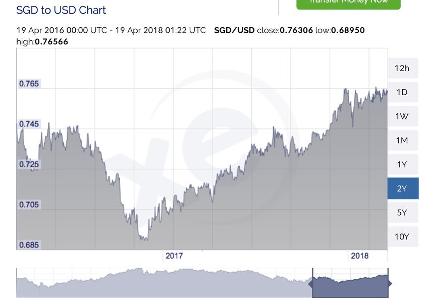
An example of Valuation can be shown with the CNY/USD exchange rate. In 2015, the
People’s Bank of China initiated the devaluation of its currency in order to promote it’s exports
and maintain it’s GDP growth. Given this devaluation and under the Valuation strategy, one
would expect this exchange rate to raise back to its fair value. Looking at Figure 2, we can see
20that after the beginning of 2017 the exchange rate starts rising, and this is exactly what we expect
by using the Valuation strategy.
Figure 2: CNY/USD Exchange Rates from April 18, 2008 to April 15, 2018 [2]
5.3.4 Fundamental
The Fundamental strategy is mostly used for cautious investors, since it relies on following
countries’ news and buy the currencies of countries of strengthening economic trends against those
with weakening economies. The difficulty behind the Fundamental method is understanding the
several economic indicators and reports, and comparing them among countries.
Throughout these sections we have an overview of how currencies are trade in the Forex market,
the types of risk prevailing as well as techniques to manage them, and the the main FX investment
strategies. With all these information, we now want to develop a forecasting model to predict the
exchange rate between the Euro and the U.S. Dollar and furthermore develop a trading strategy
to reduce risk and generate profit. We want to generate a model that incorporates all the infor-
mation and theories behind the strategies we learned in this section, but at the same time stays
parsimonious to prevent over fitting. The construction and components of this forecasting model
are described in the next section.
216 Methodology
This section describes the process followed to construct the model to predict the EUR/USD
exchange rates and the hedging strategy developed by using the predictions obtained. Here, we
start by giving an overview of the currencies selected, followed by a description of the linear
regression along with the predictor variables chosen. Next, we explain how the predictions given
from the model are improved by using another regression to fit the error. Finally, we discuss
the construction of a strategy to decide whether to enter a forward contract, or wait until the
transaction date and use the spot rate.
6.1 Currencies Selected
The currencies selected for this project are the Euro and the U.S Dollar, more specifically,
the EUR/USD exchange rate. We choose this pair given that they are both mainly affected by
macroeconomic factors, but not not affected by news or political issues, which are not modeled
into this project.
6.2 Linear Regression
The exchange rate forecast of the currency pair is obtained by developing a linear regression
using predictor variables related to the pair. In this section, we explain the methods behind a
linear regression as well as the predictor variables chosen and their connection to the currency
pair.
The linear regression model aims to understand how the response variable Y , in this case the
exchange rate of the EUR/USD, is affected by a set of predictor variables X1 , ..., Xn , which in our
case correspond to the Purchasing Power Parity (PPP) index, Basis SWAP Libor, and historical
volatility. The model is defined by the following form:
Y = β0 + β1 X1 + β2 X2 + β3 X3 + (4)
Where:
• is the value representing the error from our predictions by using the Xi ’s.
• X1 , X2 , X3 correspond to our predictor variables: PPP index, Basis SWAP Libor and histor-
ical volatility respectively.
22• β0 is the intercept and the expected value of Y when the Xi ’s are zero.
• β1 , β2 , β3 are the coefficients and corresponding slopes of X1 , X2 , X3 . In other words, βj
indicates the change in the expected value of Y by a unit change of Xj
The estimates of the β’s are the values that minimize the sum of squared errors for the sample,
which quantifies how much the data points vary around the estimated regression line.
6.2.1 Predictor Variables
Purchasing Power Parity (PPP) Index
The first predictor variable is the Purchasing Power Parity index. PPP states that exchange
rates between currencies are in equilibrium when the purchasing power is equivalent between the
two countries [18]. Thus, if the exchange rate between these two countries is equal to the ratio of
the two countries’ price level of a fixed basket of goods, then there exists an equilibrium between
these two countries. In other words, PPP explains the relation between inflation and exchange
rates, since if prices are increasing due to inflation, the country’s exchange rate needs to depreciate
to return to PPP. Therefore, one of the variables to predict a given exchange rate will be how far
the PPP index between two countries is away from an equilibrium.
Nevertheless, there are a few considerations to keep in mind when using PPP as a predictor
variable. The first one is that it only applies to tradeable goods. The second consideration is that
both countries must have comparative markets for the goods used to calculate PPP. Without this,
the difference in demand will cause prices to move without affecting the exchange rate between
these countries. Additionally, PPP does not account for legislations and transportation/transaction
costs that may cause difference in the pricing of the goods from one location to another. Finally,
it is important to acknowledge that reverting back to a PPP may take a long time, thus using this
factor as a predictor variable may not be as efficient for short-term forecasting.
The data collected to represent PPP was downloaded from the WCRS function in Bloomberg
Terminal. In general, as a rule of thumb, Bloomberg suggests that currencies over or undervalued
beyond 20% will often persist for several years before reverting. Likewise, currencies within a
10% value of their PPP estimate are considered to be fair valued. Bloomberg covers four options
to calculate Purchasing Power Parity, including Consumer, Producer, BigMac, and OECD. We
selected our base range to cover all data available, and then downloaded the data from January
2013 until December 2017 for the first two options. We then find that PPP Producer resulted in
a higher correlation with the historical exchange rates, and thus we selected this option. Finally,
23the formula used in Bloomberg to calculate PPP is given by formula (5), where the base currency
is the USD.
F oreignCP I(t) BaseCP I(average)
P P P (t) = AverageExchangeRate ∗ ∗ , (5)
F oreignCP I(average) BaseCP I(t)
CPI, or Consumer Price Index, is the monthly measurement of a country’s prices for the ma-
jority of household goods and services such as food, housing, transportation, and medical care [19].
It is calculated by taking the average of the price changes in the basket of goods (i.e, the set of
consumer products and services) [20]. Because of this, the CPI is considered a measure of inflation,
a factor that commonly affects exchange rates.
Basis SWAP Libor
We use LIBOR as our estimated interest rates for each currency. LIBOR stands for London
interbank Offered Rate, which is a benchmark rate of estimated interest rates used for short-term
loans. To calculate these rates, the banks are asked the following question: “At what rate could you
borrow funds, were you to do so by asking for and then accepting interbank offers in a reasonable
market size just prior to 11 am London time?”. Thus, it considers the lowest perceived rate at
which each bank could obtain funding in a reasonable market for a given maturity and currency.
These rates are quoted as an annualized rate (i.e. the total interest that would be paid over 365
days) with 5 decimal places, and are calculated using a trimmed arithmetic mean. This means
that the submissions are ranked in descending order and the highest and lowest 25% of them are
excluded before calculating the average in order to exclude outliers. LIBOR is also considered a
“good” measure of the “health” of the banking system and market expectation for future central
bank interest rates. LIBOR rates are calculated for different borrowing periods, such as overnight,
and one year. Nevertheless, they are only available for five currencies: USD, CHF, EUR, GBP,
and JPY.
Using the theory behind the Carry investment strategy, one of the factors selected to predict the
EUR/USD exchange rate movement is the difference between interest rates of these two currencies.
In general, we want to buy the currency with the high interest rate and sell the one with a low
interest rate. The data used to represent this variable in our model was also downloaded from
Bloomberg’s WCRS function under the name Basis SWAP Libor. A positive number in the data
implies that foreign interest rates were higher than the base rates for that particular period. The
fluctuation of this difference translates into one of the currencies appreciating against the other,
consequently affecting the exchange rate between these two.
24Historical Volatility
Volatility in the financial world describes how much the price of an asset, or in this case the
exchange rate of a currency pair, fluctuates over time. It is usually calculated using the standard
deviation or variance of the returns of a said asset. In general, the higher the volatility, the riskier
the asset [21]. There are two types of volatility, historical, which is derived from past behavior,
and implied volatility, which is what traders think will happen. Historical volatility is commonly
used to predict future volatility.
Volatility can be measured for minute return, hourly return, daily return, monthly return, or
longer time frames returns. An intraday trader may measure volatility minutely, while a long term
investor may only consider monthly volatility in a specific currency pair. In the FX market, a given
currency pair can experience higher volatility in the hours where most people are trading it, since
there is high supply and demand and the prices are moving rapidly to meet these. For example,
the EUR/USD is more volatile when when either London or New York are open, and even more
volatile when they are both open (between 1 pm and 4 pm EST).
In this model, we use the data from WCRS in Bloomberg for historical volatility of the foreign
currency versus the base currency. We neglected the implied volatility since it had a smaller
correlation with the historical exchange rates compared to the historical volatility.
6.3 Improving the model: fitting the error
Recall the linear regression from the previous section:
Y = β0 + β1 X1 + β2 X2 + β3 X3 + (6)
For the next model, we attempt to decrease the error term () by implementing another linear
regression using a momentum signal as the predictor variable. This way, we aim to fit the error
from the last regression model by generating a new regression of the form:
= λ0 + λ1 S + η (7)
Where:
• is the error of the prediction from the previous section
• S corresponds to our predictor variable, momentum.
• λ0 is the intercept and the expected value of when the S is zero.
25• λ1 is the coefficient and corresponding slope of S. In other words, λ1 indicates the change in
the expected value of by a unit change of S
• η is the new error of the model
Therefore, our combined model is:
Y = β0 + β1 X1 + β2 X2 + β3 X3 + λ0 + λ1 S + η (8)
Predictor variable: Momentum
Following the concept of momentum, we choose our predictor variable to be the crossover of two
exponentially weighted moving averages (EWMA) of different length of the EUR/USD exchange
rates, in order to fit the error found from the last model.
An EWMA is an infinite impulse response filter with exponentially decaying weights. This
approach is used when there is a belief that recent data points are more relevant than past ones,
and thus are given more weight. The following formula shows the recursive calculation.
X0
t=0
EW M At (X, α) = (9)
α ∗ Xt + (1 − α) ∗ EW M At−1 (X, α)
t>0
Where:
• Xt is the EUR/USD exchange rate at time t
• α is the weighting coefficient
• EW M At is the value of the EWMA at any time period t.
To generate the momentum signal, we used the MATLAB function tsmovavg:
output = tsmovavg(vector,’e’,timeperiod) (10)
Here, the first input is a vector, corresponding to the historical exchange rates for the currency
pair, followed by the letter ‘e’, representing the method of exponentially weighted moving average,
and finally the timeperiod, calculated using the formula shown below.
2
α= (11)
timeperiod + 1
26The two timeperiods we chose for the short (ms) and long (ml) EWMA’s are 2 and 3, corre-
sponding to α’s of 33.33% and 25%. Once we computed these two averages, we subtracted the
long EWMA (ml) from the short EWMA (ms), resulting in the vector sml. Here, positive values
in the vector indicate a positive trend (i.e. there was an upward movement in the short time vs.
the long time), while negative values represent a negative trend. A value of 0 denotes the crossover
of the short and long EWMA’s, meaning a change of direction in the trend. The timeperiods were
chosen by trial and error, looking at the behavior of the short-minus-long vector and selecting a
pair of α’s that resulted in the maximum number of crossovers. Therefore, our predictor variable
for the new model corresponds to the short-minus-long vector.
6.4 Constructing a Strategy with the Predicted Values
As an application of the predictions generated by the linear regression, we compared each of
them to the corresponding forward rates with one month expiration date and either waited for
the next month or entered a forward contract depending on which one is lower. This way, if the
forward rate is greater or equal to the predicted rate, we choose to not enter the forward contract
and wait until the next month to use the spot rate then. On the other hand, if the forward rate is
smaller than the predicted rate we enter the forward contract. Here our payoff could be either 0,
meaning what investor actually pays the spot exchange rate in one month, for our first case. Or
the payoff would be the difference between the spot rate at the moment and the forward rate of
the transaction for the second case.
For example, if we wanted to compare the prediction for November 2015, we would look at the
forward rate of the currency standing on October 2015 and with a one month expiration. For this
date in particular, we find that the predicted EUR/USD exchange rate is 1.06, while the forward
rate is 1.12. This means that in the first case, we would have to pay $1.06 in order to get 1 Euro,
and in the second case we would pay $1.12 to get 1 Euro. Therefore, according to this particular
prediction, we would prefer to wait until the next month to exchange USD for EUR rather than
settling for a forward contract, since we believe that it will be cheaper to make this exchange later.
Then, at the expiration date, we will receive a payoff of $0, since the transaction will be using the
spot rate.
On the other hand, in June 2015, the predicted rate is 1.11 and the forward rate is 1.10,
therefore, we choose to lock the forward contract this month. Then, when July comes, we look
at the actual exchange rate and find that it is actually 1.12, which means that by entering the
forward contract we prevented a loss of 0.02 USD.
We repeat this process for the predicted exchange rates and the one month forward rates from
27January 2014 until December 2017, looking at the difference between these rates and deciding if
we should wait until the next month or enter the forward contract.
We obtained the Forward rates from the Bloomberg terminal using the function FRD. The
pricing date selected was a specific month starting from December 2013, and using this as our
base, we obtained the forward prices for the next month, January 2014. We repeated this process
to obtain the one-month forward rates until December 2017.
287 Results
In this section we will summarize the results obtained by using the two models previously
described. We will discuss the fitness of the models as well as the accuracy and application of the
predictions.
7.1 Predicting the EUR/USD Currency Pair
7.1.1 Regression Analysis
As explained in the previous section, a linear regression follows the following form:
EU R/U SD = β0 + β1 X1 + β2 X2 + β3 X3 + (12)
After obtaining all the data from our predictor variables and the response variable, we used
MATLAB to generate a linear regression fitting this data and obtained the results shown in Table
3 (see the MATLAB code in the A Appendix):
Table 3: Linear Regression Results
Thus, adding the corresponding coefficients and the intercept, the linear regression for this set
of data is given by the following:
Y = 1.2788 + 0.009284X1 − 0.005067X2 + 0.001088X3 (13)
29The β coefficient represents the degree of change in the outcome variable for every unit of
change in the corresponding predictor variable. A positive sign of β implies that there is a positive
correlation, thus the exchange rate will increase by the value of the given β for every unit increase
of its predictor variable. On the other hand, a negative value means that the exchange rate will
decrease by the value of the given β for every unit increase of its predictor variable. Looking at
the β’s, we have that both the PPP and the historical volatility hold a positive correlation with
our dependent variable. On the other hand, the β corresponding to the Basis SWAP Libor rates
is negative, meaning that by every unit increase of this predictor, the exchange rate will decrease
by a value of 0.005067.
Correlation Coefficient/R-squared
The coefficient of determination (R-squared) measures the strength of the linear relationship
between two variables. R-squared can be interpreted as the percent of variance in the outcome
that can be explained by the given set of predictor variables. In this case, we calculated R-squared,
between the 4 years of exchange rates and the values obtained from our regression over this time
period. The formula used to calculate R-squared is given by calculating the SSE and the SSTO,
see formula (16). SSE is the sum of squared error and quantifies how much the data points yi vary
around the estimated regression line ybi . On the other hand, SSTO is the total sum of squares,
which quantifies how much the data points yi vary around their mean y.
N
X
SSE = (yi − ybi )2 (14)
i=1
N
X
SST O = (yi − y)2 (15)
i=1
SSE
R − squared = 1 − (16)
SST O
In general, the higher the R-squared, the better the variance in the outcome can be explained by
the given set of predictor variables. For this model, we find an R-squared value of 0.979, meaning
that 97.9% of the variance in the exchange rates can be explained by our set of predictor variables.
P-value
The p-value found by running a linear regression corresponds to the answer to the question
"how likely are we to get an extreme test statistic t as we would get if the null hypothesis were
30true?". To answer this question, we first need to run a t-test for testing the correlation. The
null hypothesis for this scenario corresponds to the correlation having a value of zero, while the
alternative hypothesis is that the correlation is not equal to zero. After running the test statistic
and finding the p-value, there are two possible conclusions. If the p-value is greater than the given
significance level (α), we fail to reject the null hypothesis and conclude that "there is not enough
evidence at the (α) level to conclude that there is a linear relationship between the predictor
variable and the response variable". On the other hand, if the p-value is smaller than the given
significance level (α), we reject the null hypothesis and conclude that "there is sufficient evidence
at the α level to conclude that there is a linear relationship between the predictor variable and the
response".
For this project in particular, we use a significance level of 0.05, and thus a p-value below 0.05
indicates that we reject the null hypothesis and that there is sufficient evidence to conclude that
there is a linear relationship between the predictor and response variables. According to Table
3, we can see that all three predictor variables’ p-value fall under 0.05. Therefore, all three of
them hold linear relationships with the response variable. Moreover, we can see that the model is
significant with a p-value of 6.11e-37
Residuals
Figure 3 shows a histogram of the Raw Residuals obtained from the linear regression from
January 2013 to December 2016. Here we can see that the residuals follow a normal distribution
and fall between -0.05 and 0.04.
Figure 3: Residuals from initial model
31You can also read