Supplementary data - Report 34: COVID-19 Infection Fatality Ratio: Estimates from Seroprevalence

29 October 2020 Imperial College COVID-19 response team

Supplementary data - Report 34: COVID-19 Infection Fatality Ratio:
Estimates from Seroprevalence
Nicholas F Brazeau1, Robert Verity1, Sara Jenks2, Han Fu1, Charles Whittaker1, Peter Winskill1, Ilaria
Dorigatti1, Patrick Walker1, Steven Riley1, Ricardo P Schnekenberg3, Henrique Hoeltgebaum4, Thomas A
Mellan1, Swapnil Mishra1, H Juliette T Unwin1, Oliver J Watson1, Zulma M Cucunubá1, Marc Baguelin1,
Lilith Whittles1, Samir Bhatt1, Azra C Ghani1, Neil M Ferguson1, Lucy C Okell1十.

1
 MRC Centre for Global Infectious Disease Analysis & WHO Collaborating Centre for infectious Disease
Modelling; Abdul Latif Jameel Institute for Disease and Emergency Analytics (J-IDEA), School of Public
Health, Imperial College London, UK
2
 Department of Clinical Biochemistry, Royal Infirmary of Edinburgh, Edinburgh, UK
3
 Nuffield Department of Clinical Neurosciences, University of Oxford
4
 Department of Mathematics, Imperial College, London, UK

Correspondence: Dr Lucy Okell l.okell@imperial.ac.uk

SUGGESTED CITATION
NF Brazeau, R Verity, S Jenks et al. COVID-19 Infection Fatality Ratio: Estimates from Seroprevalence - SUPPLEMENT.
Imperial College London (29-10-2020), doi https://doi.org/10.25561/83545.

 This work is licensed under a Creative Commons Attribution-NonCommercial-NoDerivatives
 4.0 International License.

DOI: https://doi.org/10.25561/83545 Page 1 of 40

29 October 2020 Imperial College COVID-19 response team

1. Content:

1. Content
2. Data Extraction & Manipulation
 2.1.1 Study Screening and Selection for Inclusion
 2.1.2 Data Extraction and Collation
 2.2 Age-Based Statistical Model Derivation
 2.2.1 Daily and age-stratified deaths
 2.2.2 Incorporating serology data
 2.2.3 Extension for seroreversion
 2.2.4 Full model
3. Prior Information and Model Fitting
 3.1 Symptom Onset to Seroreversion Parameter Estimation
 3.2 Onset-Outcome Delay Distributions and Serological Test Characteristics
 3.3 Estimating Specificity: Region-based Statistical Model Description
4. Insights from Simulated Data
5. Age-Based Statistical Model Posteriors
 5.1 Posterior Parameter Estimates
 5.2 Posterior Predictive Checks
6. Estimating Specificity: Region-based Statistical Model Posteriors
 6.1 Posterior Parameter Estimates
7. Pooled IFR Calculation
8. References

DOI: https://doi.org/10.25561/83545 Page 2 of 40

29 October 2020 Imperial College COVID-19 response team

2. Data Extraction & Manipulation

2.1.1 Study Screening and Selection for Inclusion
Identification of relevant serological studies was carried out using the `SeroTracker` dashboard 1, an
ongoing and continuously updated systematic review. From `SeroTracker`, a total of 175 severe acute
respiratory syndrome coronavirus 2 (SARS-CoV-2) serological studies were screened according to a
predefined set of inclusion and exclusion criteria, the details of which are described further in
Supplementary Table 1.
After screening the studies available on SeroTracker, 10/175 were selected for inclusion. Further
information and details of these studies can be found in Supplementary Table 2. Excluded studies and the
specific reason for exclusion are included as Additional File 1.

Supplementary Table 1 - Inclusion and Exclusion Criteria for Seroprevalence Studies: We assumed that
dexamethasone treatment was considered routine clinical practice approximately one-month after the RECOVERY
trial results were released (*; PMID: 32678530). Studies conducted after the introduction of dexamethasone were
excluded, as we assumed that this change in clinical practice caused shifts in the IFR that were not comparable to
pre-treatment periods.

 Inclusion Criteria Exclusion Criteria

 ● Serosurvey in a defined geographic area ● Study participants selected based on being
 representing a national or subnational healthcare workers, having symptoms of
 geographic unit for which data on COVID COVID, referring themselves for a test or self-
 deaths in all age groups are also available up selection into the study (for example, choosing
 to the date of the serosurvey. to go for an antibody test in a clinic or
 ● Sampling framework is defined. responding to an advert).
 ● Sample sizes available for serosurvey, or ● Studies of outbreaks within a confined setting
 uncertainty in the seroprevalence is explicitly that does not include a representative sample
 quantified. of the general population (e.g. a school, a
 ● Sero-assay sensitivity and specificity estimates military ship).
 available. ● Studies exclusively or primarily in a narrow age
 ● At least 100 COVID-19 deaths observed in the group (e.g. school survey).
 study area by the serosurvey midpoint. ● Surveys of patients in clinical settings
 ● First date of the serosurvey is before the (assumed higher contact with health systems
 introduction and widespread use of and healthcare workers).
 dexamethasone treatment (August 17, 2020)*

DOI: https://doi.org/10.25561/83545 Page 3 of 40

29 October 2020 Imperial College COVID-19 response team

2.1.2 Data Extraction and Collation

Observed seroprevalences, disaggregated by age and location where possible, were extracted from the
manuscripts and other sources associated with the studies identified in the review. For the majority of
studies (7/10), raw counts for the number of seropositives and number tested were available and
extracted. However, this information was not available for three studies (conducted in Italy, Sweden and
Denmark) and reported seroprevalence was extracted instead, alongside the stated confidence intervals.
As a result, we used the reported confidence intervals to capture standard errors and used a logit-
transformation instead of a binomial approach in our Age-Based model likelihood (Age-Based Model
Derivation). Further uncertainties in the data extraction process include:

 ● For the Swedish study, seroprevalence data was extracted from public health reports that were
 being constantly updated and did not provide exact dates of the period in which the serostudy
 was conducted. It was therefore assumed that the serostudy was carried out in contiguous weeks
 across the study period, based on the provided figure in the report (accessed September 11,
 2020).
 ● For the second seroprevalence survey carried out in the Netherlands, information was extracted
 from a news article (reporting an approximately 5.5% seropositivity among 7,000 participants:
 Supplementary Table 2). We therefore assumed there were 385/7,000 test-positives.
 ● In 5/10 studies (Zurich, Switzerland; Denmark; Sweden; Netherlands [second time point]), the
 age-specific seroprevalences were from broad age-groups or did not overlap well with reported
 death age-groups, only a national prevalence was available, or the report did not have sufficient
 detail to extract full information on sample sizes and seroprevalence. As a result, we assumed a
 constant attack rate (seroprevalence) across age-groups for these studies.

In addition to extracting this seroprevalence data, we also collated additional data required to estimate
the IFR. These included:

(1) Daily time-series of COVID-19 deaths were preferentially obtained from the relevant Ministries of
Health and other national public health agencies (further details in Supplementary Table 2). In some
instances when this data was not available, daily deaths were extracted from the COVID-19 Data
Repository by the Center for Systems Science and Engineering at Johns Hopkins University 2,3 (and to which
we applied a lagged difference to convert the cumulative counts to daily incidence). In a limited number
of cases, Ministries of Health have retrospectively removed previously reported deaths, leading to
negative reported deaths on particular days - these observations were set to zero. This age-aggregated
data (i.e. deaths summed across age-groups) was used in the absence of age-specific COVID-19 death time
series data being available.

(2) The proportion of COVID-19 deaths occurring by age in each location, again extracted from official
reports put out by Ministries of Health and public health agencies (detailed in Supplementary Table 2).
We assume that the age distribution of deaths is constant over time.

(3) For 6/10 of studies (Denmark; England; Spain; Geneva, Switzerland; Zurich, Switzerland; New York
State, USA) the proportion of overall deaths that occured in care homes was available and extracted so
that an adjusted IFR estimate excluding these deaths could be calculated. We assumed that all deaths
attributed to care homes occurred among individuals aged 65-years or older. We assumed that
seroprevalence across different age-groups was the same in the care home population as the general
population (see main text for discussion of this).

DOI: https://doi.org/10.25561/83545 Page 4 of 40

29 October 2020 Imperial College COVID-19 response team

(3A) In the Zurich study, over 40% of the daily observed deaths recorded a single death, which resulted in
problems when rounding and trying to recalculate deaths occurring in the care homes. As a result, the
adjusted IFR estimate excluding care home deaths for Zurich was not considered.

(4) Demographic data (i.e. age-specific population counts) were obtained from Ministries of Health and
other national public health agencies (further details in Supplementary Table 2).

(5) Demographic data required in order to generate our standardized pooled IFR calculations for settings
representative of each of the World Bank Income Strata - specifically Low Income Countries (LICs), Lower-
Middle Income Countries (LMICs), Upper Middle Income Countries (UMICs) and High Income Countries
(HICs). Consistent with previous analyses that have identified the representative countries in each of these
strata 4, we selected Madagascar, Nicaragua, Grenada and Malta: information on their demographic
structure was downloaded from the United Nations World Population Prospects 2019 site 5.

Supplementary Table 2 - Data Extraction Sources: The various sources of data for each respective study (reference
numbers). For some regions, population demographic data was taken from the City Population (CP) website:
http://citypopulation.de/

 Seroprevalence & Number of
 Serovalidation Serostudy Age-Specific Time-Series Death Care Home Death
Study Location Data Timepoints Death Data Data Demographic Data Source

Brazil 6,7 1 8 8 9, CP -

 13
Denmark 10,11 4 12 14 15

England 16,17 1 18 19 20 21

Italyተ 22,23 1 22 24 25 -

Netherlands 26,27 2 28 29 30 -

Spain 31,32 3 33 33 34 15

Sweden 35,36* 8 37 38 39 -

Geneva, Switzerland 40,41 5 42 42 43 44

Zurich, Switzerland 45 2 42 42 43 44

New York State, USA 46 1 47 2,3 48 49

* Sweden seroprevalences were limited April 20 - June 12, 2020 when multiple regions were considered (Jämtland-
Härjedalen, Jönköping, Kalmar, Skåne, Stockholm, Uppsala, Västerbotten, Västra Götaland, and Örebro). These
provinces include the majority of the Swedish population and were assumed to be nationally representative.
ተ
 Serovalidation data has not yet been released for the Italy study. As a result, serovalidation data from a comparable
study in San Francisco, USA, which used the same Abbot seroassay, were used as priors for the regional model and
re-estimation of the test sensitivity and specificity.

DOI: https://doi.org/10.25561/83545 Page 5 of 40

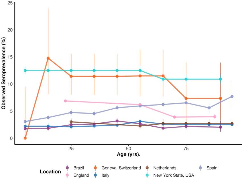
29 October 2020 Imperial College COVID-19 response team

Supplementary Figure 1 - Seroprevalence versus Age: Observed seroprevalence by age (mean age within each age-
group plotted) and binomial proportion 95% confidence intervals for the seven studies where age-specific
information was reported. With the exception of the Italian study (where reported seroprevalences and confidence
intervals are plotted), the results presented are based on the raw number of individuals seropositive and number
tested. The results of the latest seroprevalence survey are plotted among locations where multiple seroprevalence
surveys had been conducted (except for the Netherlands where age specific seroprevalence was only available in
the first survey). In our analysis we assumed a uniform seroprevalence across age-groups among the remaining three
studies included that did not contain age-specific seroprevalence data.

DOI: https://doi.org/10.25561/83545 Page 6 of 40

29 October 2020 Imperial College COVID-19 response team

2.2 Age-Based Statistical Model Derivation
2.2.1 Daily and age-stratified deaths
For individuals who die following infection, we assume that the time from infection to death follows a
gamma distribution with shape and rate . If an individual is infected at time then the probability that
they die at time is:

We make the simplifying assumption that time is discrete and measured in days, defining ( | ) to be the
probability of death on day ∈ ℤ>0 given infection at the start of day ∈ ℤ>0 where ≤ :

(the +1 term in the above comes about because we assume infections occur at the start of the day, but
deaths can be registered until the end of the day, hence (1|1) returns a positive value).

Our population is split into different age strata, each with their own probabilities of infection and death.
Let there be ∈ ℤ>0 age groups in total, and let be the proportion of the total population in age group
 ∈ 1: . In the simplest model we would expect infections to occur in a given age group in proportion to
the number of people in that group. To allow for variation in age-specific attack rates, and in order to fit
to age-specific seroprevalence data, we include a multiplicative attack rate scalar within each group,
allowing the final attack rate to be higher or lower than expected from proportions alone. Hence the
overall probability of infection in age group , which will be written , is given by:

Once infected, the probability of death in age group (i.e. the IFR in this age group) is defined as .
Hence, the overall probability of an individual in age group dying on day given infection on day can
be written ( | ).

Our raw data do not consist of individual-level outcomes, but rather aggregate counts. Specifically, two
marginal distributions were available for each study: 1) daily counts of the number of COVID-19 deaths,
summed over all age groups, and 2) the cumulative number of COVID-19 deaths at a single point in time,
but broken down by age. Both marginal distributions were fit within a single statistical framework.

Let be the number of new SARS-CoV-2 infections in the population on day . The true infections curve
is unknown, and was modelled using an exponentiated natural cubic spline, subject to the constraint that
the total number infected (i.e. the area under the curve) could not exceed the total population size . It
follows from the definitions above that the number of infections in age group on day is given by ,

DOI: https://doi.org/10.25561/83545 Page 7 of 40

29 October 2020 Imperial College COVID-19 response team

and the number of ultimately fatal infections is given by . The expected total deaths on day ,
denoted , is obtained by summing over all age groups and all possible times of infection as follows:

The observed number of COVID-19 deaths on day , denoted , is assumed to be Poisson distributed
around this expectation:

The likelihood for this part of the model is simply the product of Poisson probabilities over all days in our
time series:

Moving on to the second marginal distribution, the expected cumulative deaths in age group up until
time can be written:

These expected values are converted into expected proportions of deaths in each age group as follows:

Finally, the observed cumulative COVID-19 deaths up until day , denoted by the vector with elements
 for ∈ 1: , are assumed to be multinomially distributed with these proportions:

This is the second component of the likelihood:

2.2.2 Incorporating serology data
The third data type used in fitting comes from serological studies. For a given individual infected on day 
we model the probability of having seroconverted by day using the following formula:

where is a binary variable that equals 1 if the individual has seroconverted and 0 otherwise. This is
equivalent to assuming seroconversion with a constant hazard 1/ . Translating to the population level,

DOI: https://doi.org/10.25561/83545 Page 8 of 40

29 October 2020 Imperial College COVID-19 response team

the expected number of people to have seroconverted by time in age group , denoted , , is given
by:

This can be translated to an expected proportion via the expression , / , where is the total
population size in age group , such that ∑ =1 = .

The observed prevalence of seropositive individuals (the seroprevalence) is expected to deviate from this
proportion due to both sampling effects and imperfect test characteristics. If ∈ [0,1] is the sensitivity of
the test and ∈ [0,1] is the specificity then the test-adjusted expected seroprevalence, , , can be
calculated using the classic Rogan-Gladen correction 64:

Let the total number of people tested on day in age group be denoted , , and let the observed
number of seropositives be denoted , . We model the observed counts as binomially distributed around
the Rogan-Gladen-corrected proportion:

Finally, the likelihood for this component of the model is the product of the binomial probability over all
age groups, and over all serology study dates :

2.2.3 Extension for seroreversion
As part of a sensitivity analysis, we allowed for individuals to “serorevert” over time under an assumption
of natural waning antibodies. We assumed that individuals experience a constant hazard 1/ of
seroconverting, followed by a probability of seroreverting characterized by a Weibull distribution with
shape and scale . Under these conditions, the probability of being seropositive by the end of day 
following infection on day is given by:

All subsequent steps are identical to those described above in equations (12)-(15), resulting in an
alternative version of the likelihood component ℒ3 .

DOI: https://doi.org/10.25561/83545 Page 9 of 40

29 October 2020 Imperial College COVID-19 response team

2.2.4 Full model
The full likelihood is the product of the individual likelihood components listed above:

3. Prior Information and Model Fitting

3.1 Symptom Onset to Seroreversion Parameter Estimation

We estimated the time to seroreversion (i.e. becoming antibody negative), from previously published
longitudinal Abbott SARS-CoV-2 IgG assay data collected among non-hospitalized participants with real-
time PCR-confirmed SARS-CoV-2 infections 50. We chose to estimate seroreversion times from the Abbott
assay, as it showed the most striking decline in sensitivity over time compared to other serological assays
50
 . As a result, we present the most conservative IFR estimates with respect to the effects of seroreversion
(i.e. the number of previously infected individuals, the IFR denominator, is inflated due to assumed
“reverted” infections) to highlight the differences between estimates of IFR with and without the
assumption of seroreversion to the greatest degree. All included participants had relatively mild COVID-
19 disease and were not hospitalised. Of the 97 convalescent participants analyzed, three participants
had missing information on days post-symptoms and were excluded. Of the remaining 94 participants, six
did not seroconvert during follow-up (i.e. they were negative at baseline and remained so during the
follow-up period). Among the final 88 participants, 62 were female and the median age was 48.5 years
(range: 21 - 65 years). Seronegative status (i.e. the outcome) was defined as titres below an optical density
of 1.4 50.

To estimate the time of seroreversion after symptom onset, we fit a Weibull survival model using interval
censoring to account for the uncertainty in the observed time of seroreversion. As a comparison to our
parametric fit, we also fit a Kaplan-Meier survival curve with interval-censoring. Models were fit using the
`survival` R-package 51,52. The `survminer` R-package was used in plotting the Kaplan-Meier survival curve
(Figure 1A) 53.
From the Weibull survival model, we found that the Weibull shape and scale parameters were 3.67 and
143.7, respectively. In order to conform with the mathematical derivation of the model (Equation 16
above), we subtracted 13.3 (days) from the Weibull scale parameter to account for the time of symptom
onset to seroconversion (as an approximation) 54.

3.2 Onset-Outcome Delay Distributions and Serological Test Characteristics
The delay from onset of symptoms to death was assumed to follow a gamma distribution with a mean of
14.8 days and coefficient of variation of 0.85 (unpublished data from the COVID-19 Hospitalisation in
England Surveillance System and Public Health England). The delay from onset of symptoms to
seroconversion was assumed to follow an exponential distribution with a mean time of seroconversion of
13.3 days 54. For both distributions, the incubation period was assumed to be fixed at five days 55,56,
thereby providing overall means of onset of infection to death and seroconversion of 19.8 and 18.3 days,
respectively. Priors for the onset-delay means were truncated Gaussian distributions while the onset-to-
death coefficient of variation had a Beta distributed prior (Supplementary Table 3). When seroreversion
was considered, the prior for rate of seroreversion after seroconversion was assumed to have a truncated
Gaussian distribution (Supplementary Table 3).

DOI: https://doi.org/10.25561/83545 Page 10 of 40

29 October 2020 Imperial College COVID-19 response team

The prior distributions for the sensitivity and specificity were assumed to follow Beta distributions with
the number of true positives that were correctly identified considered for sensitivity, and the number of
true negatives correctly identified considered for specificity, among the total number of samples tested
(Supplementary Table 3). To allow for some uncertainty -- even among studies that found 100% specificity
during serovalidation -- we added 0.5 to our Beta scale and shape parameters (the Jeffreys prior;
Supplementary Table 3). For the subset of studies where regional seroprevalence information was
available (6/10), we used the posterior estimates of sensitivity and specificity from the region-based
models without time delays to re-inform the priors for the age-based IFR model. The new Beta distribution
shape parameters were calculated from the regional-based model sensitivity and specificity posteriors
using a method of moments approach with `fitdistplusr` R-package 57 (Supplementary Table 7).
The prior distributions for the age-specific IFR estimates were assumed to be uniform with minimum and
maximum values of 0% and 40%, respectively. The 40% maximum was selected as not more than three-
times the upper credible interval of three early IFR studies 58–60 (Supplementary Table 3).
Spline curves were fit with five knots to estimate the incidence of infections over time, with uniform priors
on the x- and y-axis positions. The minimum and maximum values of the y-axis positions were zero and
the total population size, while the maximum x-axis position was allowed to range from fourteen days
prior to the last observed death date and the last observed death date, respectively (Supplementary Table
3).
To estimate the proportion of infections occurring in each age group, we assumed that the attack rate
was proportional to the population fraction within that age group multiplied by an additional scaling
parameter assumed to follow a truncated Gaussian distribution (Supplementary Table 3). The modelled
seroprevalence by age was fit to the age specific seroprevalence data. Given that serostudies were
conducted over a given timeframe (e.g. two-weeks), we took the average of the model seroprevalences
over the serostudy time-period to propagate uncertainty in collection times. These modelled prevalences
were then compared with the reported seroprevalence.
Models were fit using Metropolis-Coupled Markov Chain Monte Carlo (MC3) with the `drjacoby` R package
61
 . For each model, 10,000 burnin-in and 10,000 sampling iterations with 50 rungs across 10 chains were
considered. The thermodynamic power between rungs was sequentially ranged from 5.0 to 2.5 for all sites
except England and Spain, where the thermodynamic power was ranged from 5.0 to 3.5, to ensure high
swap rates. Model convergence was assessed by analyzing the acceptance rate between rungs,
visualization of chains, and a Gelman-Rubin’s convergence diagnostic lower than 1.1 62.

DOI: https://doi.org/10.25561/83545 Page 11 of 40

29 October 2020 Imperial College COVID-19 response team

Supplementary Table 3 - Prior Distributions used in Age-Specific Model: For each parameter, the prior distribution
is indicated alongside the parameter count. For the age-specific infection fatality ratios (IFRs), younger age-groups
were reparameterized as relative risk to the oldest age group in order to improve model mixing. Similarly, the spline
knots were reparameterized relative to the last observed day, where E was the last observed day and E-14 was
fourteen days prior. The first knot was always fixed at one to allow for a common time origin. The spline y-positions
were similarly set relative to the third y-position, which was allowed to range between zero and the approximate
size of the population (popN).

 Parameter Count Distribution

 Age-Specific IFRs Number of Age Groups Uniform(0,1); Uniform(0, 0.4)

 Knots 5 Uniform(0,1); Uniform(E-14, E)

 Spline Y-Positions 5 Uniform(0,1); Uniform(0, popN)

 Attack Rate Noise Scalars Number of Age Groups Truncated-Normal(1, 0.05)
 Bounds: 0.5, 1.5

 Mean of Onset from Infection to 1 Truncated-Normal(18.3, 0.1)
 Seroconversion Bounds: 16, 21

 Mean of Onset from Infection to 1 Truncated-Normal(19.8, 0.1)
 Death Bounds: 18, 20

 Coefficient of Variation of Onset from 1 Beta(2550, 450)
 Infection to Death

 Weibull Shape Pattern for 1 Truncated-Normal(3.67, 0.5)
 Seroreversion Bounds: 2, 5

 Weibull Scale Pattern for 1 Truncated-Normal(130.4, 0.1)
 Seroreversionn Bounds: 127, 133

DOI: https://doi.org/10.25561/83545 Page 12 of 40

29 October 2020 Imperial College COVID-19 response team

3.3 Estimating Specificity: Region-based Statistical Model Description

An adapted version of the statistical model described above was used to estimate serological test
specificity in six studies where data were available by region within the larger serosurvey, as described in
the main text. The underlying assumption is that deaths in each region are proportionally related to the
true cumulative incidence in the region, estimated by seroprevalence, after adjusting for serological test
performance. As before, we incorporated test sensitivity and specificity into this model using the reported
validation data from each study as priors, and we then estimated regional and age-specific
seroprevalence, specificity, sensitivity and deaths. The age-specific IFRs were assumed to be the same in
each region, but incorporated region-specific demography so that the overall regional IFRs could vary (e.g.
London, England has a much younger population than the rest of the country, and therefore a lower
overall IFR). The delays from onset-death and onset-seroconversion were removed for analytical
tractability, and we used cumulative mortality data up to the midpoint of the serosurvey, making the
assumption that most deaths and seroconversion had occurred by the time of the serosurvey. This
assumption is reasonable for serosurveys conducted some weeks after the first wave of the epidemic. We
did not have seroprevalence data broken down by both age and region at the same time, but we fit the
model to both the marginal age and regional seroprevalence, assuming the same risk ratios of being
seropositive by age in all regions. We did not include seroreversion in this analysis. The model was fit with
`RStan` using 4 chains, each having 10,000 burn-in and 10,000 sampling iterations 63. Convergence was
assessed by visualizing the posterior distributions as well as requiring Gelman-Rubin’s convergence
diagnostic lower than 1.1 62. The underlying code is available on Github (mrc-
ide/reestimate_covidIFR_analysis/analyses/Rgn_Mod_Stan) .

DOI: https://doi.org/10.25561/83545 Page 13 of 40

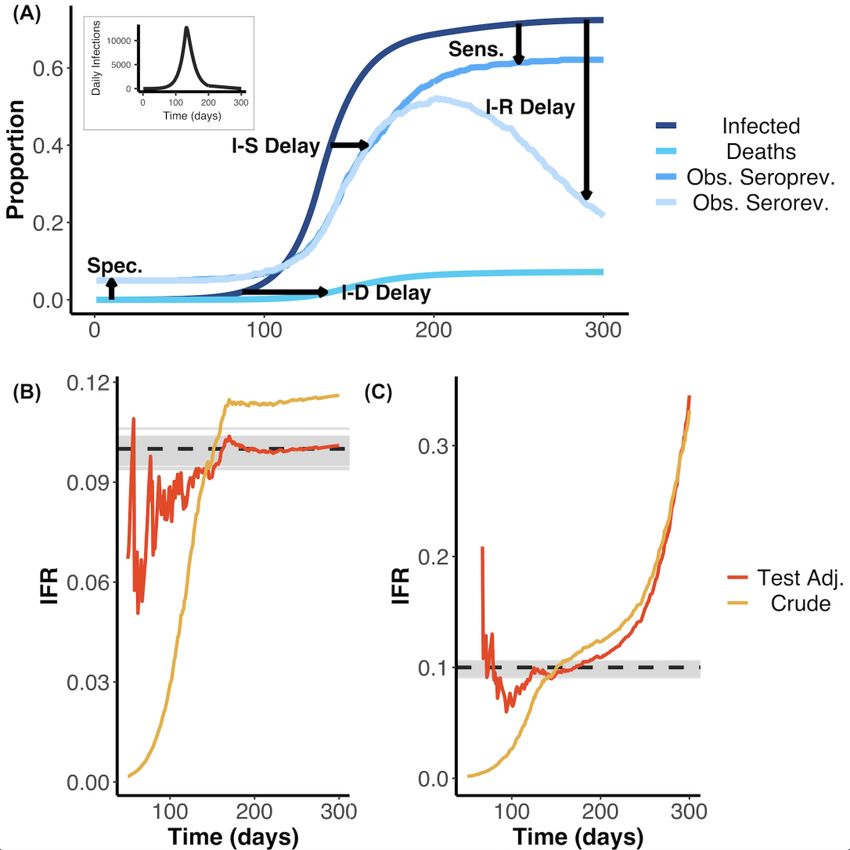
29 October 2020 Imperial College COVID-19 response team

4. Insights from Simulated Data
Accurate inference of the IFR based on serological data is challenging due to a number of factors that can
bias estimates away from the true value. These factors include: (1) the delay between infection and death,
(2) the dynamical process of seroconversion and seroreversion, and (3) serological test characteristics --
all of which are expected to interact leading to complex effects on the IFR. In order to understand how
these factors might bias the IFR, and understand the extent to which they could be disentangled, we first
developed a statistical simulator that modelled these factors and their respective effects on the IFR.

From simulations assuming seroconversion without seroreversion, we found that the crude IFR tended to
underestimate the true IFR when the epidemic was growing, or overestimate the true IFR when the
epidemic was contracting. Moreover, even after adjusting the IFR for test performance using the Rogan-
Gladen correction, a common approach to adjust for test sensitivity and specificity 64, the true IFR was
only captured when the epidemic was nearly over (Supplementary Figure 2A). These biases result from
failing to account for the delays from onset of infection to death and seroconversion. When considering
the possibility of seroreversion after seroconversion, we found that after the epidemic peaked, both the
crude IFR and the tested-adjusted IFR increasingly overestimated the true IFR as more time passed from
the first wave of the epidemic to when the serological study was undertaken (Supplementary Figure 2B).
This underestimation is expected, since reducing seroprevalence deflates the denominator (i.e. total
number infected) while the numerator (i.e. cumulative deaths) remains constant or increases.

Following our better understanding of these biases, we developed a statistical framework that accounted
for onset-outcome delay distributions alongside serologic test characteristics (e.g. specificity, sensitivity,
and the duration of the serosurvey). We found that our model allowed for correct inference of the
simulated true IFR when the potentiality for seroreversion was not and was considered (Supplementary
Figure 2). Full details on this Age-Based model framework and its mathematical derivation are detailed
above.

DOI: https://doi.org/10.25561/83545 Page 14 of 40

29 October 2020 Imperial College COVID-19 response team

Supplementary Figure 2: (A) Schematic illustrating how the effects of the various factors needed to correctly infer
the IFR can bias crude and test-adjusted (Test Adj.) estimates of the IFR. Factors shown include delays from infection
to death (I-D), to seroconversion (I-S), and to seroreversion (I-R) as well as serological test sensitivity (Sens), and
specificity (Spec). Seroprevalence was simulated from days 145-155 and 195-205 using a serologic test with 95%
specificity and 85% sensitivity and assuming that 0.1% of the total population was sampled. These simulations,
without and with seroreversion, were used as the inputs for the results displayed in panels (B) and (C). The daily
infection curve used as input for the simulation is shown as the plot inset. (B) Estimated IFR over time based on
fitting a statistical model to the simulated data that does not include seroreversion. Here, the underlying true IFR
associated with the simulated data is indicated by the dashed black line and the grey lines indicate 100 posterior
draws from the fitted statistical model (based on the posterior probability), indicating the capacity for our model
framework to correctly recover the true IFR. Red and yellow lines represent the crude and test characteristic-
adjusted (Rogan-Gladen correction) IFR estimates, calculated as if the serosurvey had been conducted on each
respective day (after day 50). The crude IFR calculation did not include cumulative deaths in the denominator (see
main text). (C) As for (B), but fitting a model that included seroreversion instead of one that lacked this feature. The
IFR values are shown as a probability instead of a percentage. Early in the outbreak, when the true seroprevalence
is less than the false positive rate, adjusting for the serologic test characteristics can result in unstable IFR estimates.

DOI: https://doi.org/10.25561/83545 Page 15 of 40

29 October 2020 Imperial College COVID-19 response team

Supplementary Figure 2 highlights the capacity for our statistical framework to recover the true underlying
IFR for a simple epidemic. We next assessed whether our model was robust to more complex epidemic
shapes. Infection curves were simulated with three shapes: exponential (unmitigated) growth,
exponential growth followed by interventions that led to resolution of the outbreak, and exponential
growth followed by interventions that lead to a nadir but were followed by a “second wave” as
interventions were relaxed. These simulations are respectively referred to as the Exponential Growth,
Outbreak Control, and Second Wave scenarios. Simulations were assumed to have two observed
seroprevalence time points (Midday: 125 and 175, where simulated serostudies were conducted over ten
days). In each instance, we found that our age-specific IFR model was able to capture the simulated true
IFR value within the 95% credible interval when seroreversion was and was not considered
(Supplementary Figures 3-4). Overall, the model appeared to be most sensitive to the unmitigated
exponential growth scenario, where the number of infections was slightly underestimated in some
posterior draws. In some instances, this resulted in the younger age groups having IFRs that were slightly
over-estimated (e.g. 0.11-0.14% insead of 0.1%) whilst the older age-groups’ true IFR was always captured
by the 95% credible intervals. This is due to the fact that the delay of onset of infection to death results in
a “lagged” infection curve, where those infected have not yet died and there is little information to fit to
a continued exponential growth versus any other shape (e.g. a continued linear line, a plateau, etc.),
particularly when there are very few deaths in the younger age-groups.

Additionally, we show that our age-specific IFR model remains able to capture the true underlying IFR in
simulated data when only only a single serostudy day is considered, rather than the two sequential
serostudies assumed for the Supplementary Figure 3 and 4 results (Supplementary Figure 5). The results
in Supplementary Figure 5 show that the uncertainty in the IFR estimates is often increased when only a
single serostudy day is considered.

DOI: https://doi.org/10.25561/83545 Page 16 of 40

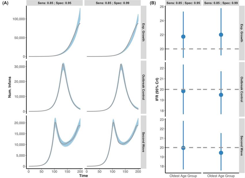
29 October 2020 Imperial College COVID-19 response team

Supplementary Figure 3 - Posterior Draws of Several Epidemic Shapes versus Simulated Infection Curve without
Seroversion: (A) Using simulated data, we created three outbreak scenarios where individuals who seroconverted
could not serorevert: exponential growth, outbreak control, and second wave (grey lines are simulated infection
input) under two different serological tests (Sensitivity: 85%; Specificity 95% vs. Sensitivity: 85%; Specificity 99%).
The blue shading represents 100 posterior draws (based on the posterior probability) of the modelled infection curve
(using an exponentiated natural cubic spline), where draws were selected based on their posterior probability. (B)
The inferred median and 95% credible intervals (blue) versus the simulated true IFR (grey, dashed line) for each of
the scenarios under the two serological test characteristics. Overall, the model accurately captures both the
simulated infection curve and the simulated IFR despite complex epidemic shapes. For all epidemic scenarios
considered, we assume that there are two seroprevalence surveys that range over days 120-130 and 170-180 and
that 0.1% of the population was sampled.

DOI: https://doi.org/10.25561/83545 Page 17 of 40

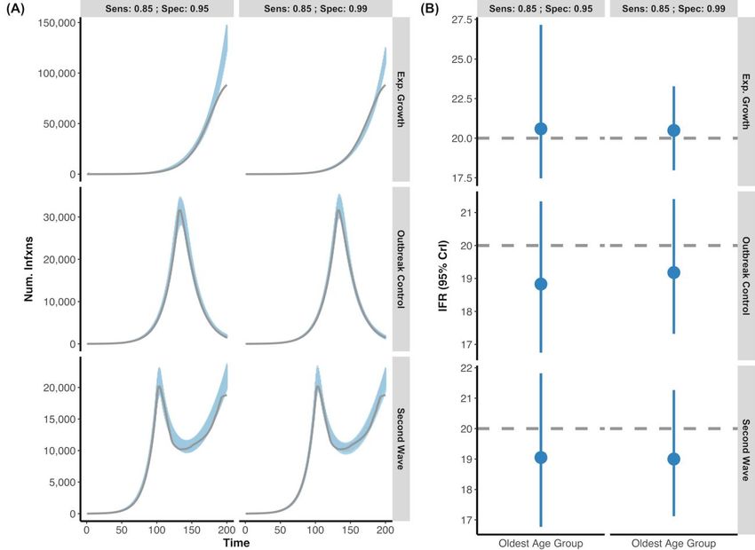
29 October 2020 Imperial College COVID-19 response team

Supplementary Figure 4 - Posterior Draws of Several Epidemic Shapes versus Simulated Infection Curve with
Seroversion: (A) Simulated data representing the same three outbreak scenarios featured in Supplementary Figure
3 (exponential growth, outbreak control, and second wave) were generated, but now with the additional feature
that individuals who seroconverted could potentially serorevert. Grey lines indicate the simulated true infection
curve under two different serological tests (Sensitivity: 85%; Specificity 95% vs. Sensitivity: 85%; Specificity 99%).
The blue shading represents 100 posterior draws (based on the posterior probability) of the modelled infection curve
(using an exponentiated natural cubic spline), where draws were selected based on their posterior probability. (B)
The inferred median and 95% credible intervals (blue) versus the simulated true IFR (grey, dashed line) for each of
the outbreak scenarios with respect to the two different serological test characteristics. As above, the model
accurately captures both the simulated infection curve and the simulated IFR while accounting for the potentiality
of seroreversion. For all epidemic scenarios considered, we assume that there are two seroprevalence surveys that
range over days 120-130 and 170-180 and that 0.1% of the population was sampled.

DOI: https://doi.org/10.25561/83545 Page 18 of 40

29 October 2020 Imperial College COVID-19 response team

Supplementary Figure 5 - Comparison of the Number of Serosurveys: Data was simulated for three age-groups
(ma1, ma2, ma3) with IFRs of 0.1%, 1%, and 10%, respectively. Follow-up time was assumed to be 200-days. The
simulations differed in the number of serological time points considered (i.e. simulated serosureys) with (A)
consisting of a single serosurvey ranging from days 145-155 versus (B) consisting of two serosurveys: days 120-130
and 170-180, respectively. In both simulations, we assume that 0.1% of the population was sampled and that the
simulated serologic test had a sensitivity and specificity of 0.85% and 0.95%, respectively. Although both models
capture the true simulated IFR values in the 95% credible intervals (grey) for each age group, there is greater
uncertainty when only a single serosurvey is considered. The IFR values are shown as a probability instead of a
percentage.

DOI: https://doi.org/10.25561/83545 Page 19 of 40

29 October 2020 Imperial College COVID-19 response team

5. Age-Based Statistical Model Posteriors

5.1 Posterior Parameter Estimates

Supplementary Table 4- Overall IFR Estimates when Standardized by Population Demography and Inferred Attack
Rates: The overall IFR estimates were calculated by standardizing for demography and the inferred attack rate,
following the definition from the age-based model (columns 3-4) or by standardizing for solely the demography and
assuming the same attack rate in each age-group (columns 5-6). Generally, the overall IFRs were very similar
between the two approaches with England as a notable exception, where the lower attack rate in the oldest age
group (consistent with the seroprevalence data) drove down the IFR.

 Pop.-Attack Rate Pop.-Attack Rate Pop. Standardized
 Standardized Standardized Modelled IFR Pop. Standardized
 Modelled IFR without Modelled IFR with without Modelled IFR with
 Seroreversion (95% Seroreversion (95% Seroreversion (95% Seroreversion (95%
Study Location Crude IFR (95 CI%) CrI) CrI) CrI) CrI)

Brazil 0.99 (0.92, 1.06) 1.03 (0.93, 1.17) 0.99 (0.89, 1.13) 1.05 (0.95, 1.21) 1.01 (0.91, 1.17)

Denmark 0.33 (0.23, 0.48) 0.53 (0.37, 1.01) 0.52 (0.37, 0.99) 0.53 (0.38, 1.02) 0.52 (0.37, 0.98)

England 1.41 (1.38, 1.45) 1.18 (0.99, 1.34) 1.04 (0.84, 1.19) 1.53 (1.26, 1.79) 1.34 (1.07, 1.55)

Italy 2.3 (1.94, 2.72) 2.53 (2.31, 2.77) 2.23 (2.03, 2.45) 2.53 (2.3, 2.79) 2.23 (2.02, 2.46)

Netherlands 0.6 (0.58, 0.63) 0.62 (0.58, 0.68) 0.59 (0.55, 0.66) 0.62 (0.58, 0.68) 0.6 (0.56, 0.66)

Spain 1.12 (1.08, 1.16) 1.14 (1.08, 1.22) 1.07 (1.01, 1.14) 1.04 (0.97, 1.12) 0.98 (0.91, 1.05)

Sweden 0.68 (0.46, 1) 1.03 (0.88, 1.37) 0.99 (0.84, 1.35) 1.03 (0.87, 1.37) 0.99 (0.84, 1.36)

Geneva, Switzerland 0.48 (0.42, 0.56) 0.49 (0.42, 0.59) 0.48 (0.4, 0.58) 0.52 (0.43, 0.63) 0.5 (0.42, 0.61)

Zurich, Switzerland 0.51 (0.45, 0.58) 0.52 (0.41, 0.67) 0.5 (0.39, 0.64) 0.53 (0.41, 0.67) 0.5 (0.39, 0.65)

New York State, USA 0.75 (0.74, 0.76) 0.77 (0.72, 0.83) 0.75 (0.7, 0.8) 0.82 (0.77, 0.89) 0.8 (0.74, 0.86)

DOI: https://doi.org/10.25561/83545 Page 20 of 40

29 October 2020 Imperial College COVID-19 response team

Supplementary Table 5 - Delay Distribution Posteriors: The posterior 95% credible intervals (CrI) for the mean delay
from infection onset to seroconversion (Serocon.) and death as well as the coefficient of variation (Coeff. of
Variation) for the onset of infection to death gamma distribution are shown for each study when seroversion was
not and was considered. Similarly, the mean of the onset from seroconversion to seroreversion (Serorev.) posterior
distribution is given for fits where seroreversion was modelled.

 Onset to Death
 Model Onset to Serocon. Onset to Death Mean Coeff. of Variation Serocon. to Serorev.
Study Location Consideration Mean (95% CrI) (95% CrI) (95% CrI) Mean (95% CrI)

Brazil Without Serorev. 18.3 (18.11, 18.5) 19.76 (19.56, 19.95) 0.85 (0.84, 0.86)

Brazil With Serorev. 18.3 (18.1, 18.49) 19.76 (19.57, 19.95) 0.85 (0.84, 0.86) 132.97 (132.85, 133)

Denmark Without Serorev. 18.3 (18.1, 18.5) 19.8 (19.61, 19.97) 0.85 (0.84, 0.86)

Denmark With Serorev. 18.3 (18.11, 18.5) 19.8 (19.61, 19.97) 0.85 (0.84, 0.86) 132.88 (132.37, 133)

England Without Serorev. 18.3 (18.11, 18.5) 19.79 (19.59, 19.96) 0.87 (0.85, 0.88)

England With Serorev. 18.3 (18.1, 18.5) 19.79 (19.59, 19.96) 0.87 (0.85, 0.88) 132.95 (132.71, 133)
Italy Without Serorev. 18.3 (18.1, 18.5) 19.87 (19.69, 19.99) 0.86 (0.85, 0.87)
Italy With Serorev. 18.3 (18.11, 18.5) 19.87 (19.69, 19.99) 0.86 (0.85, 0.87) 132.93 (132.61, 133)

Netherlands Without Serorev. 18.31 (18.11, 18.51) 19.8 (19.6, 19.96) 0.85 (0.84, 0.86)

Netherlands With Serorev. 18.31 (18.11, 18.51) 19.8 (19.6, 19.97) 0.85 (0.84, 0.86) 130.4 (130.21, 130.6)

Spain Without Serorev. 18.29 (18.1, 18.49) 19.71 (19.53, 19.88) 0.84 (0.83, 0.85)

Spain With Serorev. 18.3 (18.11, 18.49) 19.71 (19.52, 19.88) 0.84 (0.83, 0.85) 132.26 (129.24, 132.97)

Sweden Without Serorev. 18.3 (18.11, 18.5) 19.79 (19.6, 19.96) 0.85 (0.84, 0.86)
Sweden With Serorev. 18.3 (18.11, 18.5) 19.79 (19.6, 19.96) 0.85 (0.84, 0.86) 130.41 (130.21, 130.6)

Geneva, Switzerland Without Serorev. 18.3 (18.11, 18.5) 19.77 (19.57, 19.95) 0.85 (0.84, 0.86)

Geneva, Switzerland With Serorev. 18.3 (18.11, 18.5) 19.77 (19.57, 19.95) 0.85 (0.84, 0.86) 130.4 (130.21, 130.6)

Zurich, Switzerland Without Serorev. 18.3 (18.1, 18.49) 19.79 (19.59, 19.96) 0.85 (0.84, 0.86)

Zurich, Switzerland With Serorev. 18.3 (18.1, 18.49) 19.79 (19.6, 19.96) 0.85 (0.84, 0.86) 130.4 (130.21, 130.6)

New York State, USA Without Serorev. 18.3 (18.1, 18.49) 19.74 (19.55, 19.94) 0.87 (0.86, 0.89)

New York State, USA With Serorev. 18.3 (18.1, 18.49) 19.75 (19.55, 19.93) 0.87 (0.86, 0.88) 132.81 (131.98, 132.99)

DOI: https://doi.org/10.25561/83545 Page 21 of 40

29 October 2020 Imperial College COVID-19 response team

Supplementary Table 6- Age Specific Estimates of the Infection Fatality Ratio across Included Studies: The age-
specific IFR estimates (without standardization) are provided with 95% credible intervals (CrI) for models where
seroversion was not and was considered. The crude IFRs and 95% confidence intervals (CI) are included for
comparison. In addition, the inferred observed seroprevalence -- from 100 posterior draws based on the posterior
probabilities and corrected for test sensitivity and specificity with the Rogan-Gladen equation -- is provided alongside
the observed seroprevalence for the latest serosurvey with respect to each study and age-group. Ages of “999”
indicate an upper bound.

 Age Modelled
 Group Seroprev. Observed Modelled Seroprev. Seroprev. with IFR without IFR with Serorev.
Study Location (years) Midday Seroprev. without Serorev. Serorev. Crude IFR (95% CI) Serorev. (95% CrI) (95% CrI)

Brazil (0,9] 2020-06-06 1.74 2.24 (2.07, 2.42) 2.23 (2.07, 2.42) 0.03 (0.02, 0.05) 0.03 (0.02, 0.03) 0.02 (0.02, 0.03)

Brazil (9,19] 2020-06-06 1.82 2.23 (2.09, 2.41) 2.22 (2.08, 2.39) 0.03 (0.02, 0.04) 0.02 (0.02, 0.03) 0.02 (0.02, 0.02)

Brazil (19,29] 2020-06-06 2.48 2.31 (2.16, 2.47) 2.32 (2.15, 2.51) 0.06 (0.05, 0.08) 0.07 (0.06, 0.08) 0.07 (0.06, 0.08)

Brazil (29,39] 2020-06-06 2.61 2.34 (2.17, 2.51) 2.34 (2.17, 2.48) 0.19 (0.16, 0.22) 0.2 (0.18, 0.24) 0.2 (0.17, 0.23)

Brazil (39,49] 2020-06-06 3.17 2.44 (2.3, 2.61) 2.44 (2.28, 2.63) 0.39 (0.33, 0.46) 0.49 (0.43, 0.57) 0.47 (0.41, 0.55)

Brazil (49,59] 2020-06-06 2.65 2.38 (2.24, 2.56) 2.39 (2.22, 2.56) 1.06 (0.9, 1.27) 1.17 (1.03, 1.36) 1.13 (0.99, 1.31)

Brazil (59,69] 2020-06-06 1.85 2.15 (1.98, 2.3) 2.15 (2.01, 2.29) 3.61 (2.96, 4.56) 3.18 (2.8, 3.7) 3.06 (2.67, 3.57)

Brazil (69,79] 2020-06-06 2.17 2.23 (2.08, 2.42) 2.25 (2.11, 2.43) 6.25 (4.93, 8.32) 6.31 (5.49, 7.39) 6.05 (5.27, 7.11)

Brazil (79,999] 2020-06-06 2.02 2.23 (2.02, 2.43) 2.24 (2.09, 2.45) 13.18 (9.19, 21.46) 13.47 (11.65, 16.13) 12.94 (11.22, 15.69)

Denmark (0,59] 30/04/2020 2.4 2.13 (1.9, 2.33) 2.11 (1.95, 2.39) 0.01 (0.01, 0.02) 0.02 (0.01, 0.04) 0.02 (0.01, 0.04)

Denmark (59,69] 30/04/2020 2.4 2.15 (1.89, 2.34) 2.12 (1.93, 2.39) 0.28 (0.19, 0.41) 0.45 (0.29, 0.88) 0.44 (0.28, 0.86)

Denmark (69,79] 30/04/2020 2.4 2.14 (1.88, 2.35) 2.1 (1.94, 2.4) 0.96 (0.66, 1.39) 1.57 (1.06, 3.03) 1.51 (1.03, 2.92)

Denmark (79,999] 30/04/2020 2.4 2.14 (1.86, 2.32) 2.12 (1.96, 2.37) 4.02 (2.79, 5.76) 6.76 (4.7, 13) 6.55 (4.58, 12.4)

England (0,44] 26/06/2020 6.87 6.62 (6.5, 6.78) 6.64 (6.42, 6.82) 0.02 (0.02, 0.02) 0.02 (0.02, 0.02) 0.02 (0.01, 0.02)

England (44,64] 26/06/2020 6.18 6.1 (5.91, 6.25) 6.1 (5.96, 6.23) 0.52 (0.5, 0.54) 0.45 (0.38, 0.51) 0.4 (0.32, 0.46)

England (64,74] 26/06/2020 3.89 4.38 (4.17, 4.64) 4.38 (4.23, 4.63) 3.19 (2.97, 3.45) 2.57 (2.13, 2.98) 2.25 (1.8, 2.65)

England (74,999] 26/06/2020 3.96 4.76 (4.46, 5.02) 4.8 (4.53, 5.14) 17.34 (15.75, 19.21) 15.06 (12.33, 17.82) 13.2 (10.47, 15.44)

Italy (0,9] 20/06/2020 2.2 2.41 (2.24, 2.57) 2.49 (2.3, 2.64) 0 (0, 0.01) 0 (0, 0.01) 0 (0, 0.01)

Italy (9,19] 20/06/2020 2.2 2.43 (2.21, 2.58) 2.49 (2.3, 2.7) 0 (0, 0) 0 (0, 0) 0 (0, 0)

Italy (19,29] 20/06/2020 2.1 2.39 (2.28, 2.56) 2.43 (2.27, 2.64) 0.01 (0.01, 0.01) 0.01 (0.01, 0.02) 0.01 (0.01, 0.02)

Italy (29,39] 20/06/2020 2.25 2.41 (2.26, 2.55) 2.46 (2.31, 2.63) 0.04 (0.04, 0.05) 0.04 (0.03, 0.06) 0.04 (0.03, 0.05)

DOI: https://doi.org/10.25561/83545 Page 22 of 40

29 October 2020 Imperial College COVID-19 response team

Italy (39,49] 20/06/2020 2.4 2.45 (2.28, 2.62) 2.49 (2.34, 2.65) 0.14 (0.12, 0.16) 0.15 (0.13, 0.18) 0.13 (0.11, 0.16)

Italy (49,59] 20/06/2020 3.1 2.64 (2.49, 2.77) 2.69 (2.53, 2.86) 0.4 (0.35, 0.46) 0.52 (0.46, 0.59) 0.46 (0.4, 0.52)

Italy (59,69] 20/06/2020 2.6 2.47 (2.34, 2.66) 2.54 (2.37, 2.68) 1.75 (1.49, 2.04) 2.02 (1.78, 2.3) 1.78 (1.58, 2.03)

Italy (69,79] 20/06/2020 2.5 2.47 (2.27, 2.67) 2.5 (2.34, 2.65) 5.64 (4.83, 6.55) 6.58 (5.83, 7.46) 5.82 (5.15, 6.57)

Italy (79,89] 20/06/2020 2.5 2.47 (2.32, 2.61) 2.51 (2.32, 2.66) 12.47 (10.78, 14.3) 15.72 (13.95, 17.83) 13.89 (12.27, 15.74)

Italy (89,999] 20/06/2020 2.5 2.46 (2.33, 2.6) 2.51 (2.36, 2.69) 19.44 (16.99, 22.03) 26.6 (23.56, 30.13) 23.46 (20.75, 26.66)

Netherlands (0,49] 15/05/2020 5.5 5.49 (5.14, 5.87) 5.48 (5.21, 5.75) 0.01 (0.01, 0.01) 0.01 (0, 0.01) 0.01 (0, 0.01)

Netherlands (49,59] 15/05/2020 5.5 5.38 (5.07, 5.62) 5.37 (5.04, 5.69) 0.11 (0.1, 0.12) 0.11 (0.09, 0.14) 0.11 (0.09, 0.13)

Netherlands (59,69] 15/05/2020 5.5 5.45 (5.15, 5.72) 5.39 (5.15, 5.66) 0.45 (0.41, 0.5) 0.46 (0.41, 0.53) 0.44 (0.39, 0.5)

Netherlands (69,79] 15/05/2020 5.5 5.43 (5.18, 5.7) 5.44 (5.15, 5.76) 2 (1.82, 2.21) 2.09 (1.89, 2.34) 2 (1.82, 2.25)

Netherlands (79,89] 15/05/2020 5.5 5.47 (5.14, 5.71) 5.43 (5.17, 5.75) 6.38 (5.84, 7.01) 6.98 (6.35, 7.82) 6.69 (6.09, 7.48)

Netherlands (89,999] 15/05/2020 5.5 5.42 (5.17, 5.67) 5.42 (5.11, 5.67) 10.65 (9.8, 11.65) 12.2 (10.9, 13.76) 11.7 (10.49, 13.22)

Spain (0,9] 15/06/2020 3.07 3.76 (3.58, 3.98) 3.67 (3.48, 3.87) 0 (0, 0) 0 (0, 0.01) 0 (0, 0)

Spain (9,19] 15/06/2020 3.81 4.38 (4.17, 4.56) 4.23 (4.03, 4.42) 0 (0, 0) 0 (0, 0.01) 0 (0, 0.01)

Spain (19,29] 15/06/2020 4.73 5 (4.79, 5.17) 4.86 (4.65, 5.04) 0.01 (0.01, 0.02) 0.01 (0.01, 0.02) 0.01 (0.01, 0.02)

Spain (29,39] 15/06/2020 4.54 4.91 (4.71, 5.1) 4.73 (4.56, 4.92) 0.03 (0.03, 0.04) 0.03 (0.02, 0.04) 0.03 (0.02, 0.04)

Spain (39,49] 15/06/2020 5.61 5.67 (5.55, 5.82) 5.48 (5.35, 5.67) 0.07 (0.06, 0.07) 0.07 (0.06, 0.08) 0.06 (0.06, 0.07)

Spain (49,59] 15/06/2020 5.95 5.93 (5.76, 6.1) 5.74 (5.59, 5.87) 0.21 (0.2, 0.23) 0.21 (0.19, 0.24) 0.2 (0.18, 0.22)

Spain (59,69] 15/06/2020 6.22 6.07 (5.88, 6.25) 5.87 (5.67, 6.03) 0.73 (0.67, 0.79) 0.75 (0.69, 0.81) 0.7 (0.65, 0.77)

Spain (69,79] 15/06/2020 6.52 6.18 (5.98, 6.35) 6 (5.77, 6.23) 2.46 (2.24, 2.72) 2.64 (2.44, 2.86) 2.48 (2.29, 2.69)

Spain (79,89] 15/06/2020 5.59 5.55 (5.24, 5.89) 5.39 (5.15, 5.66) 7.78 (6.76, 9.1) 8.57 (7.81, 9.47) 8.03 (7.33, 8.85)

Spain (89,999] 15/06/2020 7.71 5.56 (5.27, 5.88) 5.4 (5.14, 5.74) 10.05 (7.73, 13.85) 15.52 (13.97, 17.42) 14.56 (13.06, 16.36)

Sweden (0,9] 2020-10-06 7.1 5.57 (5.15, 5.99) 5.47 (4.96, 5.83) 0 (0, 0) 0 (0, 0.01) 0 (0, 0.01)

Sweden (9,19] 2020-10-06 7.1 5.54 (5.17, 5.96) 5.44 (5.08, 5.8) 0 (0, 0) 0 (0, 0) 0 (0, 0)

Sweden (19,29] 2020-10-06 7.1 5.58 (5.19, 5.96) 5.41 (5.16, 5.9) 0.01 (0.01, 0.01) 0.01 (0.01, 0.03) 0.01 (0.01, 0.03)

Sweden (29,39] 2020-10-06 7.1 5.59 (5.15, 5.9) 5.46 (5.1, 5.91) 0.01 (0.01, 0.02) 0.02 (0.01, 0.04) 0.02 (0.01, 0.04)

Sweden (39,49] 2020-10-06 7.1 5.54 (5.2, 5.89) 5.44 (5.11, 5.87) 0.05 (0.03, 0.07) 0.08 (0.05, 0.11) 0.07 (0.05, 0.11)

Sweden (49,59] 2020-10-06 7.1 5.57 (5.19, 5.92) 5.43 (5.04, 5.82) 0.17 (0.11, 0.25) 0.26 (0.2, 0.35) 0.25 (0.19, 0.34)

DOI: https://doi.org/10.25561/83545 Page 23 of 40

29 October 2020 Imperial College COVID-19 response team

Sweden (59,69] 2020-10-06 7.1 5.61 (5.27, 5.92) 5.42 (5.11, 5.89) 0.44 (0.3, 0.65) 0.67 (0.54, 0.91) 0.65 (0.52, 0.89)

Sweden (69,79] 2020-10-06 7.1 5.56 (5.18, 6.04) 5.45 (5.09, 5.96) 1.53 (1.05, 2.25) 2.36 (1.94, 3.17) 2.26 (1.87, 3.13)

Sweden (79,89] 2020-10-06 7.1 5.57 (5.07, 5.91) 5.47 (5.13, 5.83) 6.22 (4.33, 8.94) 10.05 (8.34, 13.51) 9.69 (8.01, 13.3)

Sweden (89,999] 2020-10-06 7.1 5.54 (5.2, 5.98) 5.42 (5.05, 5.8) 15.22 (10.93, 20.98) 27.28 (22.61, 36.67) 26.18 (21.55, 35.99)

Geneva,
Switzerland (0,9] 2020-07-05 0 9.09 (8.31, 10.09) 9.04 (8.31, 9.85) 0 (0, 0.01) 0 (0, 0.01)

Geneva,
Switzerland (9,19] 2020-07-05 14.77 9.5 (8.54, 10.33) 9.45 (8.49, 10.31) 0 (0, 0) 0 (0, 0.01) 0 (0, 0.01)

Geneva,
Switzerland (19,29] 2020-07-05 11.41 9.77 (9.13, 10.44) 9.69 (9.08, 10.35) 0 (0, 0) 0 (0, 0.01) 0 (0, 0.01)

Geneva,
Switzerland (29,39] 2020-07-05 11.41 9.73 (8.86, 10.53) 9.67 (8.99, 10.44) 0.02 (0.02, 0.03) 0.02 (0, 0.06) 0.02 (0, 0.06)

Geneva,
Switzerland (39,49] 2020-07-05 11.41 9.69 (8.94, 10.64) 9.68 (8.9, 10.41) 0 (0, 0) 0 (0, 0.01) 0 (0, 0.01)

Geneva,
Switzerland (49,59] 2020-07-05 11.49 9.14 (8.39, 10.16) 9.19 (8.45, 10.31) 0.11 (0.08, 0.16) 0.12 (0.05, 0.21) 0.11 (0.05, 0.2)

Geneva,
Switzerland (59,69] 2020-07-05 11.49 9.1 (8.32, 10.06) 9.11 (8.44, 10.01) 0.26 (0.19, 0.39) 0.28 (0.15, 0.45) 0.27 (0.14, 0.44)

Geneva,
Switzerland (69,79] 2020-07-05 7.34 8.99 (8.02, 9.77) 8.91 (8.26, 9.76) 1.75 (1.01, 4.53) 1.28 (0.91, 1.74) 1.24 (0.88, 1.69)

Geneva,
Switzerland (79,999] 2020-07-05 7.34 8.84 (8.09, 9.71) 8.8 (7.98, 9.7) 9.33 (5.55, 21.53) 7.42 (6.03, 9.26) 7.18 (5.82, 8.96)

Zurich,
Switzerland (0,9] 16/05/2020 1.59 1.54 (1.38, 1.68) 1.55 (1.39, 1.72) 0 (0, 0) 0.01 (0, 0.02) 0.01 (0, 0.02)

Zurich,
Switzerland (9,19] 16/05/2020 1.59 1.54 (1.4, 1.71) 1.55 (1.37, 1.7) 0 (0, 0) 0.01 (0, 0.02) 0.01 (0, 0.02)

Zurich,
Switzerland (19,29] 16/05/2020 1.59 1.54 (1.38, 1.68) 1.54 (1.38, 1.68) 0 (0, 0) 0.01 (0, 0.02) 0.01 (0, 0.02)

Zurich,
Switzerland (29,39] 16/05/2020 1.59 1.54 (1.4, 1.69) 1.54 (1.39, 1.69) 0 (0, 0) 0.01 (0, 0.01) 0.01 (0, 0.01)

Zurich,
Switzerland (39,49] 16/05/2020 1.59 1.54 (1.41, 1.69) 1.53 (1.38, 1.69) 0 (0, 0) 0.01 (0, 0.01) 0.01 (0, 0.01)

Zurich,
Switzerland (49,59] 16/05/2020 1.59 1.52 (1.42, 1.66) 1.54 (1.38, 1.7) 0.12 (0.08, 0.18) 0.11 (0.02, 0.24) 0.11 (0.02, 0.24)

DOI: https://doi.org/10.25561/83545 Page 24 of 40

29 October 2020 Imperial College COVID-19 response team

Zurich,
Switzerland (59,69] 16/05/2020 1.59 1.54 (1.42, 1.69) 1.55 (1.38, 1.71) 0.42 (0.3, 0.64) 0.42 (0.19, 0.73) 0.4 (0.18, 0.69)

Zurich,
Switzerland (69,79] 16/05/2020 1.59 1.54 (1.4, 1.67) 1.54 (1.41, 1.72) 0.91 (0.66, 1.39) 0.93 (0.52, 1.45) 0.89 (0.5, 1.39)

Zurich,
Switzerland (79,999] 16/05/2020 1.59 1.52 (1.36, 1.72) 1.54 (1.35, 1.66) 7.35 (5.42, 10.82) 8.01 (6.03, 10.53) 7.68 (5.82, 10.16)

New York 12.25 (11.81,
State, USA (0,9] 23/04/2020 12.49 12.26 (11.95, 12.71) 12.69) 0 (0, 0) 0 (0, 0) 0 (0, 0)

New York 12.27 (11.87,
State, USA (9,19] 23/04/2020 12.49 12.26 (11.81, 12.62) 12.71) 0 (0, 0) 0 (0, 0) 0 (0, 0)

New York 12.26 (11.86,
State, USA (19,29] 23/04/2020 12.49 12.27 (11.76, 12.73) 12.74) 0.02 (0.02, 0.02) 0.02 (0.02, 0.02) 0.02 (0.02, 0.02)

New York
State, USA (29,39] 23/04/2020 12.49 12.24 (11.89, 12.7) 12.27 (11.89, 12.7) 0.07 (0.07, 0.07) 0.07 (0.06, 0.08) 0.07 (0.06, 0.08)

New York 12.34 (11.86,
State, USA (39,49] 23/04/2020 12.49 12.25 (11.86, 12.75) 12.73) 0.2 (0.19, 0.22) 0.21 (0.19, 0.23) 0.2 (0.18, 0.23)

New York
State, USA (49,59] 23/04/2020 12.49 12.26 (11.88, 12.69) 12.3 (11.85, 12.7) 0.51 (0.48, 0.54) 0.53 (0.48, 0.58) 0.51 (0.47, 0.56)

New York
State, USA (59,69] 23/04/2020 10.89 11.12 (10.62, 11.61) 11.22 (10.79, 11.7) 1.4 (1.3, 1.5) 1.41 (1.29, 1.56) 1.37 (1.25, 1.51)

New York 11.26 (10.65,
State, USA (69,79] 23/04/2020 10.89 11.2 (10.71, 11.84) 11.69) 3.05 (2.85, 3.28) 3.13 (2.85, 3.46) 3.04 (2.77, 3.35)

New York 11.15 (10.65,
State, USA (79,999] 23/04/2020 10.89 11.18 (10.74, 11.68) 11.72) 7.2 (6.74, 7.71) 7.73 (7.05, 8.53) 7.51 (6.84, 8.25)

DOI: https://doi.org/10.25561/83545 Page 25 of 40

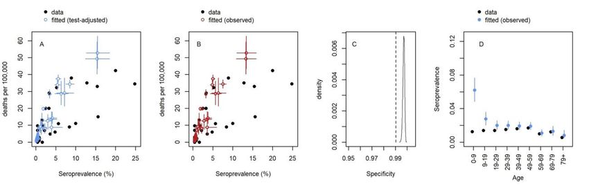
29 October 2020 Imperial College COVID-19 response team

5.2 Posterior Predictive Checks

Supplementary Figure 6 - Posterior Draws of Modelled Seroprevalence without Seroreversion for the Oldest Age-
Group: Results are presented from the statistical modelling framework where seroreversion was not included. For
each study and its associated model fits, we selected 100 posterior draws of the modelled true seroprevelance
(yellow) based on their posterior probabilities. Due to space constraints, we only show here the results for the oldest
age group, although younger age-groups showed similar results. Given this true inferred seroprevalence, the
expected observed seroprevalence, with the Rogan-Gladen correction, is also displayed (blue). The observed
seroprevalence for the oldest age group is indicated along with its 95% confidence interval are indicated in black
with the serostudy time-period demarcated by a grey box. The 95% confidence intervals were calculated using a
binomial proportion with the exception of the Denmark, Italy, and Sweden studies, where reported seroprevalences
and confidence intervals are plotted (binomial counts were not available). Overall, observed seroprevalences
matched closely with modelled seroprevalence and varied in some instances due to the modelled differences in the
distributions of infections across age-groups (Supplementary Table 6).

DOI: https://doi.org/10.25561/83545 Page 26 of 40

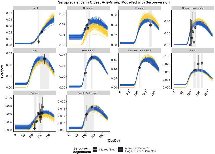
29 October 2020 Imperial College COVID-19 response team

Supplementary Figure 7 - Posterior Predictive Check: Inferred Deaths without Seroreversion for the Oldest Age-
Group: Results are presented from the statistical modelling framework where seroreversion was not included. For
each study and its associated model fits we selected 100 posterior draws of the modelled IFR and delay of infection
onset to death based on the posterior probabilities (grey). Inferred deaths were projected forward in time according
to the gamma distribution fit and compared to the age-specific time-series deaths (i.e. model input: blue). Due to
space constraints, we only show here the results for the oldest age group, although younger age-groups showed
similar results.

DOI: https://doi.org/10.25561/83545 Page 27 of 40

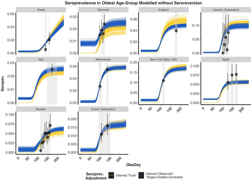
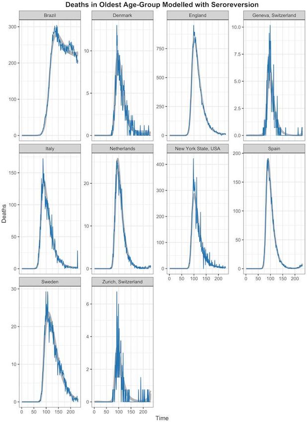
29 October 2020 Imperial College COVID-19 response team

Supplementary Figure 8 - Posterior Draws of Modelled Seroprevalence with Seroreversion for the Oldest Age-
Group: Results are presented from the statistical modelling framework where seroreversion was explicitly included.
The seroreversion sensitivity analysis was used to present a conservative estimate of the IFR, as we assumed a fast
rate of antibody waning from the Abbott assay ( Muecksch et al. 2020). For each study and its associated model fits
we selected 100 posterior draws of the modelled true seroprevelance (yellow) according to the posterior
probabilities. Due to space constraints, we only show here the results for the oldest age group, although younger
age-groups showed similar results. The rate of seroreversion after seroconversion was estimated from previously
published data on the Abbott SARS-CoV-2 IgG assay, which demonstrated the greatest decay of sensitivity over time
among the four assays evaluated (Muecksch et al. 2020). Given the true inferred seroprevalence, the expected
observed seroprevalence, with the Rogan-Gladen correction, is also displayed (blue). Overall, observed
seroprevalences matched closely with modelled seroprevalence and varied in some instances due to the modelled
differences in the distributions of infections across age-groups (Supplementary Table 6). The effect of seroreversion
later in the pandemic is apparent, particularly in Italy.

DOI: https://doi.org/10.25561/83545 Page 28 of 40