Evaluation of the SEdiment Delivery Distributed (SEDD) Model in the Shihmen Reservoir Watershed - MDPI
←
→
Page content transcription
If your browser does not render page correctly, please read the page content below
sustainability

Article
Evaluation of the SEdiment Delivery Distributed
(SEDD) Model in the Shihmen Reservoir Watershed
Kent Thomas 1 , Walter Chen 1, * , Bor-Shiun Lin 2            and Uma Seeboonruang 3, *
 1    Department of Civil Engineering, National Taipei University of Technology, Taipei 10608, Taiwan;
      t107429401@ntut.edu.tw
 2    Disaster Prevention Technology Research Center, Sinotech Engineering Consultants, Taipei 11494, Taiwan;
      bosch.lin@sinotech.org.tw
 3    Faculty of Engineering, King Mongkut’s Institute of Technology Ladkrabang, Bangkok 10520, Thailand
 *    Correspondence: waltchen@ntut.edu.tw (W.C.); uma.se@kmitl.ac.th (U.S.);
      Tel.: +886-2-27712171 (ext. 2628) (W.C.); +66-2329-8334 (U.S.)

 Received: 3 June 2020; Accepted: 30 July 2020; Published: 2 August 2020

 Abstract: The sediment delivery ratio (SDR) connects the weight of sediments eroded and transported
 from slopes of a watershed to the weight that eventually enters streams and rivers ending at
 the watershed outlet. For watershed management agencies, the estimation of annual sediment yield
 (SY) and the sediment delivery has been a top priority due to the influence that sedimentation has
 on the holding capacity of reservoirs and the annual economic cost of sediment-related disasters.
 This study establishes the SEdiment Delivery Distributed (SEDD) model for the Shihmen Reservoir
 watershed using watershed-wide SDRw and determines the geospatial distribution of individual
 SDRi and SY in its sub-watersheds. Furthermore, this research considers the statistical and geospatial
 distribution of SDRi across the two discretizations of sub-watersheds in the study area. It shows
 the probability density function (PDF) of the SDRi . The watershed-specific coefficient (β) of SDRi is
 0.00515 for the Shihmen Reservoir watershed using the recursive method. The SY mean of the entire
 watershed was determined to be 42.08 t/ha/year. Moreover, maps of the mean SY by 25 and 93
 sub-watersheds were proposed for watershed prioritization for future research and remedial works.
 The outcomes of this study can ameliorate future watershed remediation planning and sediment
 control by the implementation of geospatial SDRw /SDRi and the inclusion of the sub-watershed
 prioritization in decision-making. Finally, it is essential to note that the sediment yield modeling can
 be improved by increased on-site validation and the use of aerial photogrammetry to deliver more
 updated data to better understand the field situations.

 Keywords: sediment delivery distributed model; sediment yield; SEDD; sediment delivery ratio; β
 coefficient; Shihmen Reservoir watershed

1. Introduction
      Land degradation has been confirmed as a threat to agricultural productivity worldwide [1].
The gradual dissipation of quality topsoil transported as sediments along hill slopes and deposited into
rivers and reservoirs has impacted multiple agricultural areas across the world. Sediment delivery by
soil erosion and landslides has also led to the decreased longevity and failure of reservoirs and other
water infrastructure. Moreover, due to the importance of reservoirs and dams to the water security
of large populations in the developed world, the impact of sedimentation has been highlighted as
a major issue in need of research worldwide over the past half a century and into the future. These
processes influence many of the United Nations’ (UN) Sustainable Development Goals (SDGs) [1–3].
Heavy sustained sedimentation leads to a severe influence on industries and economic growth for

Sustainability 2020, 12, 6221; doi:10.3390/su12156221                       www.mdpi.com/journal/sustainability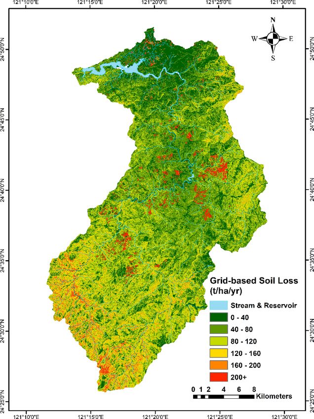
Sustainability 2020, 12, 6221                                                                    2 of 21

agriculture-based communities (SDG 8, 9, 10), the sustainability of cities and communities (SDG 11),
and the availability of clean water downstream (SDG 6). These processes also pollute rivers, streams,
and the sea by the transport of chemicals with sediments damaging marine flora and fauna and
influencing the sustainability of marine environments (SDG 14).
      Southeast Asia presents an even more advanced dilemma as the environmental and
geomorphological characteristics across the region displays a strong influence on the rate of soil
erosion, and the region’s population and economies are already suffering from the impact [1]. After
Typhoon Gloria impacted Taiwan, the Shihmen reservoir watershed was one of the many watersheds
heavily inundated by sediments from soil erosion and landslides. This event was an example of
typhoon events affecting Taiwan due to its tropical monsoon climate. The impact of these events creates
frequent and high magnitude sediment disasters and long-term sediment inundation. The effect of
extreme meteorological events on Shihmen and other reservoirs and the threat to urban and agricultural
water supply quality throughout the nation has encouraged the Government of Taiwan to facilitate
soil conservation research and countermeasures within the watershed through the introduction of soil
conservation policies and programs. Taiwan’s geographical location places it in a precarious position
that geomorphologically has a high frequency of highly erodible soil materials and, additionally, its
tropical monsoon climate brings frequent extreme rainfall or typhoon events which have led to massive
sediment loads, dissociated by mass movements, and soil erosion, to be transported from slopes of
watersheds into rivers and streams, affecting water supply in many communities. These events increase
the siltation of reservoirs, such as the Shihmen Reservoir in Northern Taiwan, which diminishes
the country’s capacity to sustainably manage its water supply and poses a threat to the long-term
sustainability of the dam and the populations it serves [4,5].
      Therefore, sediment modeling and monitoring in Taiwan is of paramount importance to improve
watershed conservation and sustainable water management by understanding how sediments are
dissociated, translocated, and transported down the slopes of watersheds, entering streams as massive
sediment loads. These sediments deposit along the waterway with detrimental impacts to river flow
and along slopes, increasing future sediment disaster hazards and clogging reservoirs and dams,
affecting water supplies to nearby populated districts and farms.

1.1. Sediment Delivery Ratio (SDR)
     Researchers have established that the sediment yield (SY) and siltation found in rivers and
dams are not equivalent to the gross sediments that have dissociated from the slopes through land
degradation processes. The sediment delivery ratio (SDR) was established as the relationship between
the SY and the gross erosion (A, in some research denoted as Soil Loss, SL). The SDR acts as a reducer
to equate the maximum amount of soil erosion to the sediments delivered to the outlet. SDR is
a continuous variable with a range from zero to one. In the initial stages of soil erosion research,
SDR was evaluated for an entire watershed and a single outlet, such as a reservoir, denoted as SDRw .
However, as computational power has improved and research methods have become more developed,
SDR is discretized to sub-watersheds, micro watersheds, and even more minute hydrological units
within a watershed. This has been denoted as a geospatial SDRi and is defined as the fraction of
the gross soil loss (SL) from the hydrological unit, i, that reaches a flow pathway [6].
     Many methods for determining the SDR have been developed over the past six decades. Long-term
monitoring of SY in test plots and different regions were the starting point in SDR research and
established multiple geophysical and hydrological factors that affect SDR. Wu et al. [7] stated that
there are three prominent methods of estimating SDR, which are: (1) the ratio between soil erosion and
sediment yield, (2) empirical formula relationships between SDR and its contributing factors, and (3)
spatial modeling and numerical modeling using hydraulic and hydrological theories. These include
models for the calculation and classification of SDR based on regional and local observed data.
     Li [8] determined from the comparison of the USLE results and the outlet sediments at the Shihmen
Reservoir that the SDR was 0.49 from the annual siltation amount of 71.2 t/ha/year (between 2011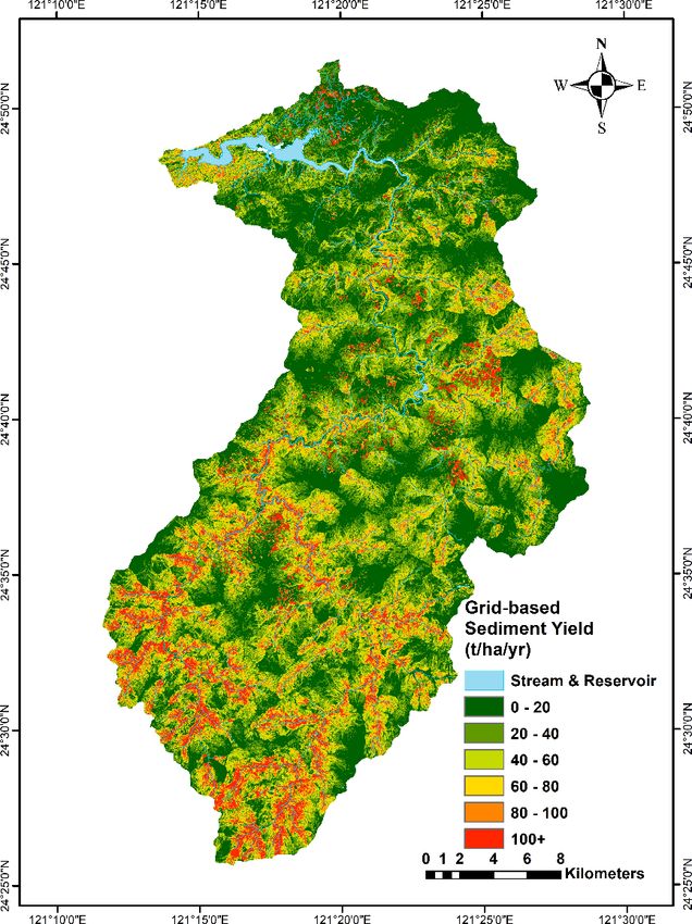
Sustainability 2020, 12, 6221                                                                        3 of 21

and 2015), which includes sheet and rill erosion, gully erosion, and landslides. There have been
other studies of the SDR in the Shihmen Reservoir watershed but these have mainly focused on
the post-landslide erosion SDR or event-based SDR. Tsai et al. [9] defined the SDR of the landslide
areas in the watershed from 0.42 to 0.78 for eroded areas and zero for areas where aggradation
occurred. Moreover, Tsai et al. [10] employed the model of Bathurst et al. [11] of the sediment delivery
of landslides. They determined that the sediment delivery of landslides in the Shihmen Reservoir
watershed ranged from 0.75 to 0.89 (1986–1998), 0.48 to 0.64 (1998–2004), and 0.40 to 0.58 for typhoon
Aere (2004). Lin et al. [12] explored the impact of different factors (such as curve number and Manning’s)
on the SDR in the Shihmen Reservoir watershed.
      SWCB [13] previously employed DEMs of difference (DoD) method to determine a correlation
between SDR and the entire watershed (SDRw ) in the Shihmen Reservoir watershed and concluded
the relationship to be SDR = 41.23WArea    −0.017 where W
                                                           Area is the watershed area, and the SDRw was
0.368. Chen et al. [14] used the Grid-based Sediment Production and Transport Model (GSPTM) to
determine SDRw to be 0.299 (rounded to 0.30) for a simulation of the impact of the Typhoon Morakot on
the Yufeng and Xiuluan sub-watersheds, and Chiu et al. [15] extended the GSPTM to identify unstable
stream reaches. Additionally, Liu [16] determined that the total soil loss (also commonly-termed gross
soil erosion or the total amount of soil erosion) was 90.6 t/ha/year by converting measured average
erosion depth of erosion pins [17,18] to the amount of soil erosion. This study emphasizes the SDR of
recent years and assumes SDRw = 0.49.

1.2. Spatial Discretization
      This research compares the implementation of the SEDD with grid–cell unit analysis across
the watershed and two discretization levels of sub-watersheds (25 and 93 SW). Spatial discretization of
watersheds in hydrological models has been a critical issue for many researchers within the remote
sensing, physical modeling, hydrology, and mathematical computations fields [19]. Wood et al. [20]
elaborated that watersheds are areas made of infinite minute points of related hydrological processes (for
example, evaporation, infiltration, and runoff). Watersheds can be further divided into sub-watersheds
or sub-basins that are continuous assemblages or spatial objects that drain towards a specific point,
contains similar vegetation layers and/or linked slope, or elevation characteristics, and are commonly
used in the study of landslides, soil erosion, hydrology, and other natural processes and are specific
areas within a watershed. There are many methods of defining watersheds, sub-watersheds, and even
more minute forms of discretization, such as hydrological units depending on the characteristics of
the areas [19–22].
      Contextually, at the time of the development of many soil erosion models and concepts
from the 1970s to the 1990s, computational cost, time, and power were limitations that hindered
the discretization of watersheds to more elements [19]. Therefore, many older models were developed
with sub-watershed as the smallest hydrological unit. This has continued even to the 2000s with
the SWAT (Soil and Water Assessment Tool) model, and research has supported the object area
discretization in soil erosion, LULC (Land Use and Land Cover), and sedimentation models and has
criticized the use of areal discretization. SWAT is a comprehensive soil erosion model that is popular in
the field of hydrology. In this study, we utilized the first stage in the SWAT analysis, the discretization
of a study area into sub-basins/sub-watersheds, to develop 25-subwatershed divisions. The two inputs
used in this analysis was the surface topography and the land use type [23]. Previously in the Shihmen
Reservoir watershed, grid cells and slope units have also been employed in soil erosion research [16].
      Researchers implementing the SEdiment Distributed Delivery (SEDD) model have mainly focused
on the hydrological or morphological unit [6,24–29] but Di Stefano and Ferro [30] utilized grid cells in
the SEDD model.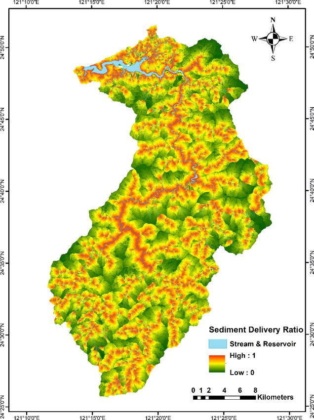
Sustainability 2020, 12, 6221 4 of 21
1.3. Study Objectives
Geomorphological changes, climate change, and land degradation processes are highly influential
to soil erosion studies. Therefore, it is important to highlight the time scale. The prioritization
of watersheds or sub-watersheds for soil erosion, landslide, and conservation works has been
a long-standing topic in geomorphology, hydrology, disaster management, and environmental planning
research. In the past, the gross soil loss (often derived by the USLE model) and its contributing factors
have been the primary focus for prioritization of soil conservation planning. This study explored
the sediment yield value to the prioritization of sub-watersheds for remediation and conservation.
This research incorporated and considered the implementation of the SEDD model in the Shihmen
Reservoir watershed and the research objectives, methods, and assumptions are as follows:
1. The main focus of this study was on the advancement of the soil erosion research in the Shihmen
Reservoir watershed to include determination of the watershed-specific coefficient, β, using
known SDRw values, and developing the SDRi relationship and SEDD model for the watershed,
applying the findings to the assessment of the sediment yield (SY) by sheet and rill erosion in
the watershed.
2. In this study, the non-point source sheet and rill erosion calculated by the USLE is the main target
land degradation process. Landslides, gully erosion, and channel type erosions are not considered.
3. The datasets employed are assumed to be from the same period and are the most recent available
data for this study area.
4. This study, additionally, explores the statistical properties of the SDR, SL, and SY of the watershed
using two sub-watershed discretizations (25 and 93) of the Shihmen Reservoir watershed and
compares the results.
5. This study determines the watershed prioritization of soil conservation using the SY determined
by the SEDD.
This study is a theoretical and statistical analysis of the SDR distribution based upon the SEDD
model using real data from the Shihmen Reservoir watershed.
2. Study Area
The Shihmen Reservoir watershed (elevation map shown in Figure 1a) is a 759.53 km2 watershed
found in Northern Taiwan between latitudes 24.426◦ N and 24.861◦ N, and longitudes 121.192◦ E
and 121.479◦ E. Local authorities use the reservoir to regulate 23% of the water supply for the nearby
communities, industries, and agriculture. The effective storage volume of the reservoir is 207 million m3 .
Still, it has been affected by heavy sedimentation, and some of the additional check dams established to
diminish sedimentation have been affected or damaged in past years. The established subdivision of
the watershed by local government is into five sub-watersheds, namely Ku-Chu, Yu-Feng, San-Kuang,
Pai-Shih, Tai-Kang sub-watersheds. However, in this study, the entire watershed is delineated
into 25 sub-watersheds (Figure 1b) and 93 sub-watersheds (Figure 1c), as explained in Section 3.1.
The watershed is traversed by the Tahan River and its irregular pattern of tributaries that spread across
the steep, high slopes of the sub-watersheds (angle 20◦ to 85◦ with an elevation between 220 m and
3527 m). The subtropical monsoon climate and the annual rainfall between 2200 mm and 2800 mm in
the watershed encourages a densely vegetated state, which is mostly natural and artificial coniferous
and broadleaved trees, and the trend in rainfall pattern has increased over the past decades to create
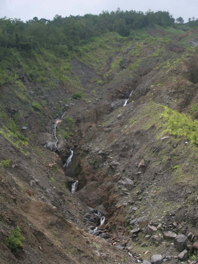
concerns of soil erosion (Figure 1d) [9,31].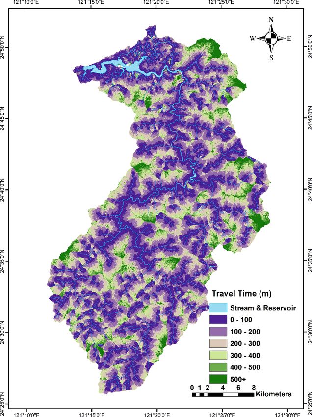
Sustainability 2020, 12, 6221                                                                                   5 of 21
Sustainability 2020, 12, x FOR PEER REVIEW                                                                      5 of 20

                                (a)                                                    (b)

                                (c)                                                    (d)

      Figure 1. Maps of the Shihmen Reservoir watershed: (a) elevation, (b) 25 sub-watersheds, and (c) 93
      sub-watersheds. (d) An illustrative picture of soil erosion.

3. Methodology
3. Methodology
      The
      The SEDD
           SEDD model
                 model developed
                        developed by  by Ferro
                                         Ferro and and Minacapilli
                                                            Minacapilli [24]
                                                                        [24] analyzes
                                                                              analyzes the
                                                                                         the spatially
                                                                                             spatially distributed
                                                                                                        distributed SY
                                                                                                                     SY
by  determining  the parameters     of SDR   and      SL    found using   any   soil loss  model.
by determining the parameters of SDR and SL found using any soil loss model. The SDR is found by    The  SDR  is found
by  a relationship
a relationship     between
               between   the the  travel
                              travel timetime
                                           (tp,i) (t
                                                  andp,i ) aand a watershed-specific
                                                             watershed-specific           coefficient,
                                                                                   coefficient,        β. β cannot
                                                                                                 β. β cannot         be
                                                                                                              be deter-
determined   analytically
mined analytically  but isbut  is determined
                            determined           iteratively,
                                         iteratively,            by balancing
                                                             by balancing        the relationship
                                                                            the relationship        between
                                                                                                between       a known
                                                                                                          a known   SY,
SY, SL,  and SDR.  The SY  is evaluated   for  the    entire   watershed    and  the  two  discretizations,
SL, and SDR. The SY is evaluated for the entire watershed and the two discretizations, 25 and 93 sub-        25  and 93
sub-watershed   models,   to compare   the  impact        of aggregation   on
watershed models, to compare the impact of aggregation on the model outputs.   the model    outputs.
     The flow chart of the SEDD model implemented in this study is distributed among four stages
as shown in Figure 2:
     Stage 1 (1.1):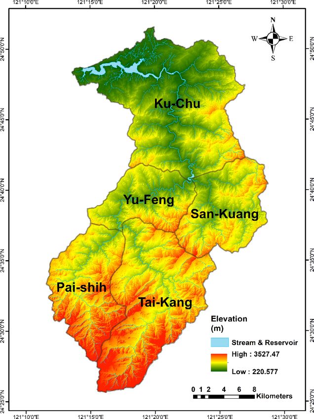
Sustainability 2020, 12, 6221                                                                     6 of 21

    The flow chart of the SEDD model implemented in this study is distributed among four stages as
shown in Figure 2:

Stage 1 (1.1):

1.      Determine the study area and input the DEM.
Sustainability 2020, 12, x FOR PEER REVIEW                                                       6 of 20
2.      Determine the slope, flow direction, and river/stream map from a derived depression-less DEM.
3.
1.      Use the flow
      Determine       direction
                 the study  areaand
                                 andriver/stream map as input to determine the flow distance, which is
                                      input the DEM.
2.      then used  with the  slope to determine the travel time.
      Determine the slope, flow direction, and river/stream   map from a derived depression-less DEM.
3.
StageUse
      2: the flow direction and river/stream map as input to determine the flow distance, which is
     then used with the slope to determine the travel time.
4.     Find the six parameters of the USLE equation and estimate SL.
     Stage 2:
5.     Determine the SDR using measured outlet SY and estimated SL.
4. Find the six parameters of the USLE equation and estimate SL.
Back to stage 1.2:
5. Determine the SDR using measured outlet SY and estimated SL.
6.     Determine
     Back to stage β from the SDR, SL, and the travel time found.
                   1.2:
StageDetermine
6.    3:        β from the SDR, SL, and the travel time found.
7.     Return
     Stage 3: to the DEM and discretize the study area into sub-watersheds/hydrological units or any
       other applicable unit of analysis.
7. Return to the DEM and discretize the study area into sub-watersheds/hydrological units or any
Stageother
      4: applicable unit of analysis.

8.    Stage 4:
        Re-estimate the SDR for the parent watershed and each sub-watershed.
9.
8.      Estimate the
      Re-estimate thesediment  yield
                      SDR for the    (SY) watershed
                                  parent  and perform any
                                                    and   further
                                                        each      analysis necessary.
                                                             sub-watershed.
9.    Estimate the sediment yield (SY) and perform any further analysis necessary.

                                Figure
                                Figure 2.
                                       2. Flow
                                          Flow chart
                                               chart of
                                                     of the
                                                         the SEDD
                                                             SEDD model
                                                                  model in
                                                                         in this
                                                                            this study.
                                                                                 study.

     SDR evaluation for SEDD modeling requires the development of three (3) main parameters: the
slope, hydraulic length, and the β coefficient. The “flow distance” module of the ArcGIS software
was employed to develop the horizontal flow paths and required the use of the “flow accumulation”
and “flow direction” modules. The slope map and other component datasets of the USLE/SEDD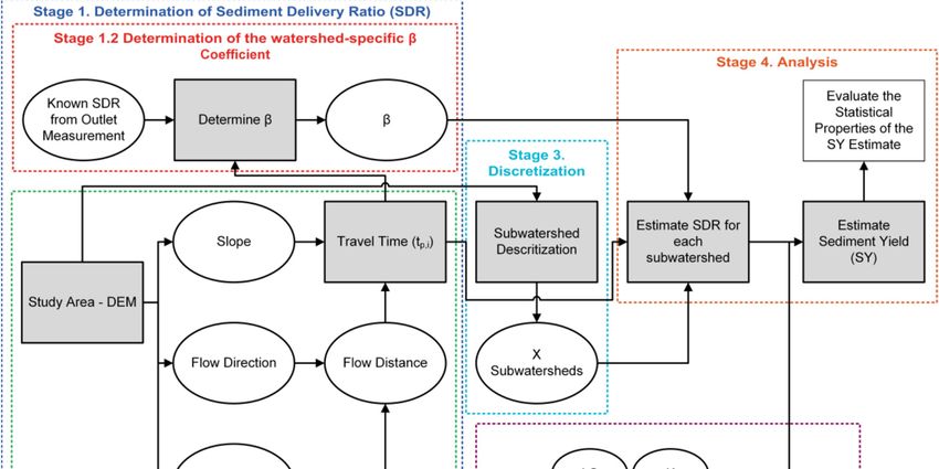
Sustainability 2020, 12, 6221 7 of 21
SDR evaluation for SEDD modeling requires the development of three (3) main parameters:
the slope, hydraulic length, and the β coefficient. The “flow distance” module of the ArcGIS software
was employed to develop the horizontal flow paths and required the use of the “flow accumulation”
and “flow direction” modules. The slope map and other component datasets of the USLE/SEDD model
were developed in the ArcGIS platform.
This study relied upon the R programming language. Specifically, the “raster,” “e1071,” and
“LaplacesDemon” libraries were employed for statistical analysis, conversion of data from raster
to point datasets, and other analysis, while the “ggplot2” libraries of R were employed for data
visualization [32–35].
The USLE model in this study was developed in the ArcGIS model builder framework updating
the model originally developed by Jhan [36], Yang [37], Li [8], and Liu [38].
The USLE model was developed by Wischmeier and Smith [39,40] and is designed to predict
the average annual SL by sheet and rill erosion. It has been continuously improved upon and localized
by many researchers over the past decades. The USLE model can be denoted as follows:
Am = Rm Km LSCP (1)
where Am is the computed soil loss per unit area (t/ha/year), Rm is the rainfall and runoff factor
(MJ-mm ha−1 h−1 year−1 ), Km is the soil erodibility factor (t-h MJ−1 mm−1 ), L is the slope-length factor
(dimensionless), S is the slope-steepness factor (dimensionless), C is the cover and management factor,
and P is the support practice factor.
3.1. Sediment Distributed Delivery Model (SEDD)
The SEDD utilizes the calculation of the flow length for SDR developed by Ferro and
Minacapilli [24], which includes considerations for slope and the roughness/runoff coefficient. SY,
the sediment yield by the annual scale, for a basin is discretized into Ni morphological units and is
measured in tonnes (t):
XNi XN i
SYi = Ami SDRi SUi (2)
i=1 i=1
where Ami is the computed soil loss per unit area (t/ha/year) for the morphological unit i, SUi is the area
of the morphological unit i (ha), and Ni is the number of morphological units over the watershed area
(dimensionless).
Ferro and Minacapilli [24] concluded that the SDRw can be physically defined using watershed
morphological data without the consideration of the soil loss model. SDRi in Equation (2) and
the relationship between the SDRw and SDRi was defined as follows (Equations (3) and (4)):
XNp λi,j
−βtp,i
lp,i
SDRi = e = exp−β √ = exp−β √ (3)
j=1
S p,i Si,j
" #
PNi lp,i
i=1
exp −β √ Ami SUi
Sp,i
SDRw = PNi (4)
A SUi
i=1 mi
where tp,i is the travel time from ith morphological unit to the nearest stream reach (m), β is the roughness
and runoff coefficient for the watershed (m−1 ), sp,i is the slope of the hydraulic flow path (m/m), lp,i is
the length of the hydraulic flow path (m), λi,j and Si,j are the length and slope of each morphological
unit i localized along the hydraulic path j, and Np is the number of morphological units localized along
the hydraulic path j [6,24,26–29].
In this study, the parent watershed (the Shihmen Reservoir watershed) was discretized into two
discrete sets of children sub-watersheds, specifically 25 and 93 sub-watersheds. The 25 sub-watersheds
were delineated using the SWAT model with the input of the DEM and river course of the Shihmen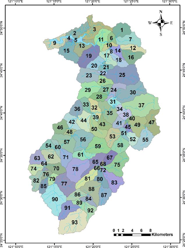
Sustainability 2020, 12, 6221 8 of 21
Reservoir watershed. The output was 25 hydrologically connected sub-watersheds, as shown in
Figure 1b. The 93 sub-watersheds were delineated using the ArcGIS Watershed module utilizing an
input of the
Sustainability flow
2020, 12, direction
x FOR PEERand a stream map derived from flow accumulation. The output was
REVIEW 8 of 93
20
hydrologically connected sub-watersheds, as shown in Figure 1c.
The SEDD
unit analysis model
is less timewas implemented
consuming as 10 mhas
to produce, grida data,
lowerwith over seven cost,
computational million
anddata
canpoints
garnerandre-
aggregated
sults that areinto sub-watersheds.
aggregated by specificThis study
areas. derivedthere
However, the grid-based SEDD model
can be discrepancies due and aggregated
to oversimplifi-
the dataset
cation, some intovast. sub-watersheds to examine the impact this can have on the output SY data.
A grid–cell-based analysis is more computationally expensive, and larger watersheds can be quite
3.2.
timeSediment
consuming Yieldor Determination
hardware-expensive but may provide alternative results. On the other hand,
the hydrological unit analysis is less time consuming to produce, has a lower computational cost, and
Flow direction (FD) algorithms estimate the flow of a specified material from a source cell (S1)
can garner results that are aggregated by specific areas. However, there can be discrepancies due to
continuously to the next neighboring cells (N1) until a stopping point or limitation point (river or
oversimplification, some vast.
stream in Figure 3) has been reached, such as a stream, river, or dam. The SDR model considers the
hydraulic
3.2. Sediment flow of sediments
Yield Determinationthrough each morphological/hydrological unit to the trunk river or its
tributaries (in this scenario, the Tahan river, and its tributaries) using the single flow direction algo-
rithm,Flow direction (FD)
deterministic algorithms
D8. The distanceestimate
traveledthe by flow of a specified
particles has been material
termed thefrom a source
“flow path cell (S1)
length”
continuously to the next neighboring cells (N1) until a stopping point
and has varying definitions and methods of calculation. The flow distance module in ArcGIS was or limitation point (river or
stream
used to in Figure
define the3) has beenflow
horizontal reached, suchtoas
distance thea river
stream, river,
using theorD8dam. The SDR model considers
flow direction.
the hydraulic flow of sediments through each morphological/hydrological
The relative time taken to reach the sink from the source has been termed unit tothe
the “travel
trunk river
time.”or
its tributaries (in this scenario, the Tahan river, and its tributaries) using the single
Moreover, Jain and Kothyari [27] state that the travel time from a cell i is equivalent to the total travel flow direction
algorithm,
time through deterministic
each of theD8. Np The
cellsdistance
along its traveled
flow pathby particles has been termed
until terminating the “flow
at a channel. The path
flowlength”
path
and has varying definitions and methods of calculation. The flow distance module
length and the slope in conjunction with a watershed-wide β coefficient are used to derive, firstly, in ArcGIS was used
to define the horizontal flow distance to the river
the travel time and, secondly, the SDR within the SEDD model. using the D8 flow direction.
Figure
Figure 3.
3. A
Aflow
flow path
path showing
showing the
the single
single flow
flow D8
D8 algorithm where SS =
algorithm where = source
source and
and N
N ==Node
Node (re-drawn
(re-drawn
from
from [41]).
[41]).
The SY was first
relative timederived
taken using a watershed-wide
to reach gridsource
the sink from the of the USLE
has beenand termed
SDRi, and thethen compared
“travel time.”
against
Moreover,theJain
discretization
and Kothyari of the
[27] 25 sub-watersheds
state that the travelmodel andathe
time from cell93
i issub-watersheds
equivalent to the model using
total travel
the
timemean, median,
through each and mode
of the for each
Np cells alongsub-watershed.
its flow path until terminating at a channel. The flow path
length and the slope in conjunction with a watershed-wide β coefficient are used to derive, firstly,
4.
theResults
travel time and, secondly, the SDR within the SEDD model.
The results
The SY was offirst derived
SEDD using ainwatershed-wide
modeling grid of the
the Shihmen Reservoir USLE and
watershed SDR
and itsi ,sub-watersheds
and then compared are
against the discretization of
shown in the following sections. the 25 sub-watersheds model and the 93 sub-watersheds model using
the mean, median, and mode for each sub-watershed.
4.1. The β Coefficient
4. Results
Using GIS, we could calculate the flow lengths, slope, and travel time needed in Equations (3)
The results of SEDD modeling in the Shihmen Reservoir watershed and its sub-watersheds are
and (4) for the Shihmen Reservoir watershed. At the same time, soil loss could be computed by USLE,
shown in the following sections.
and the SDRw is known to be 0.49 previously determined from the annual siltation of the reservoir
[8]. Therefore, the only unknown is Equation (4) was the β coefficient. By assuming an initial value
of β, we can solve for the β coefficient iteratively to satisfy the Equation (4). We found the β coefficient
to be 0.00515. This is the first result of applying the SEDD model to the Shihmen Reservoir watershed
using the iterative method, and a number like this has never been obtained before. The determined
β coefficient is watershed specific.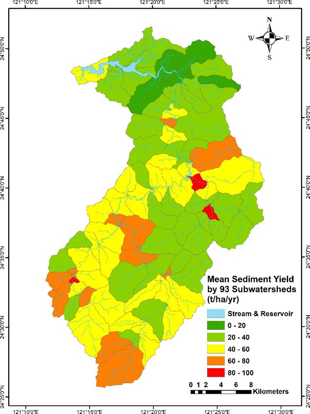
Sustainability 2020, 12, 6221                                                                         9 of 21

4.1. The β Coefficient
     Using GIS, we could calculate the flow lengths, slope, and travel time needed in Equations (3)
and (4) for the Shihmen Reservoir watershed. At the same time, soil loss could be computed by USLE,
and the SDRw is known to be 0.49 previously determined from the annual siltation of the reservoir [8].
Therefore, the only unknown is Equation (4) was the β coefficient. By assuming an initial value of β,
we can solve for the β coefficient iteratively to satisfy the Equation (4). We found the β coefficient to
be 0.00515. This is the first result of applying the SEDD model to the Shihmen Reservoir watershed
using the iterative method, and a number like this has never been obtained before. The determined β
coefficient is watershed specific.

4.2. Grid-Based Travel Time, SDR, SL, and SY
      The following Figures 4–7 depict the travel time, sediment delivery ratio (SDR), soil loss (SL), and
sediment yield (SY) determined using the SEDD model.
      The probability density functions (PDF) of the grid–cell-based SDR, SL, and SY of the Shihmen
Reservoir watershed have asymmetric, right-skewed distributions (which will be shown later in
Section 4.3 2020,
Sustainability with12,
                    two   representative
                       x FOR PEER REVIEWsub-watersheds). This study determined in the Shihmen Reservoir
                                                                                                     9 of 20
watershed for SDR: the mean value of the distribution was 0.474 (not the same as SDRw ), the median
4.2. Grid-Based
was   0.459, andTravel
                   the modeTime,was
                                 SDR,  SL, and
                                    0.317.  ForSY
                                                the SL of the entire watershed, the mean was estimated as
87.07 t/ha/year, and the median was 71.74 t/ha/year. Lastly, the mean SY for the entire watershed was
      The following Figures 4–7 depict the travel time, sediment delivery ratio (SDR), soil loss (SL),
42.08 t/ha/year, and the median was 29.80 t/ha/year.
and sediment yield (SY) determined using the SEDD model.

                                Figure
                                Figure 4.
                                       4. Travel
                                          Travel Time of the
                                                 Time of the Shihmen
                                                             Shihmen Reservoir
                                                                     Reservoir watershed.
                                                                               watershed.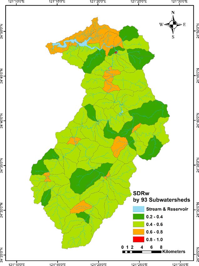
Sustainability 2020, 12, 6221                                                                         10 of 21
                                Figure 4. Travel Time of the Shihmen Reservoir watershed.

Sustainability 2020, 12, Figure 5.
                                5. Sediment
                         x FOR PEER
                         Figure      REVIEWDelivery
                                   Sediment Delivery Ratio
                                                     Ratio of
                                                           of the
                                                              the Shihmen
                                                                  Shihmen Reservoir
                                                                          Reservoir watershed.
                                                                                    watershed.        10 of 20

                  Figure 6. Soil
                            Soil Erosion/Soil
                                 Erosion/Soil Loss Distribution of the Shihmen Reservoir watershed.
Sustainability 2020, 12, 6221 11 of 21
Figure 6. Soil Erosion/Soil Loss Distribution of the Shihmen Reservoir watershed.
Sustainability 2020, 12, x FOR PEER REVIEW 11 of 20
4.3. Comparison by Sub-Watershed Discretization on SDR, SL, and SY
This study considered the distribution of SDR, SL, and SY in the Shihmen Reservoir watershed
discretized into 93 sub-watersheds. From Figure 8, it is evident that both the median and the mean
of SDR by 93 SW had Figure
very similar distributions with a central tendency centered around 0.500.
7. Sediment Yield of the Shihmen Reservoir watershed.
The range of mean SL by sub-watershed was between 15.60 t/ha/year (SW #8) and 151.21
t/ha/year
4.3. (SW #45)
Comparison and the range
by Sub-Watershed
The probability density of the(PDF)
median
Discretization
functions of
ofon SLgrid–cell-based
was
SDR,
the SL,1.15
andt/ha/year
SY SDR, (SW SL,#5) andSY
and 136.36
of thet/ha/year
Shihmen
(SW #69).
Reservoir The evaluation
watershed have of the median
asymmetric, of the SL
right-skewed for 93 SW showed
distributions that
(which the
will median
be showntended
later to
in be
sec-
This study considered the distribution of SDR, SL, and SY in the Shihmen Reservoir watershed
between
tion 4.3 60
with and
two90 t/ha/year,
representative and over 20 sub-watersheds
sub-watersheds). This had
study a median
determined between
in the 60–70 t/ha/year.
Shihmen In
Reservoir
discretized into 93 sub-watersheds. From Figure 8, it is evident that both the median and the mean of
contrast, the
watershed formean
SDR: SL
theby sub-watersheds
mean value of the were more widely
distribution spread
was 0.474 (notand
thehad
same a number of
as SDRw0.500.peaks
), the be-
median
SDR by 93 SW had very similar distributions with a central tendency centered around
tween 60 and 120 t/ha/year with over 20 sub-watersheds valued at 80 to 100 t/ha/year.
was 0.459, and the mode was 0.317. For the SL of the entire watershed, the mean was estimated as
87.07 t/ha/year, and the median was 71.74 t/ha/year. Lastly, the mean SY for the entire watershed was
42.08 t/ha/year, and the median was 29.80 t/ha/year.
(a) (b)
Figure8.8.Histograms
Figure Histogramsofofthe thedistributions
distributionsofofmeans
means and
and medians:
medians: (a)(a) sediment
sediment delivery
delivery ratio
ratio (SDR)
(SDR) and
and
(b) (b)loss
soil soilofloss
theofShihmen
the Shihmen Reservoir
Reservoir sub-watersheds.
sub-watersheds.
The
Therange
rangeofofmean SL by
the mean SYsub-watershed
by sub-watershedwas in
between 15.60 t/ha/year discretization
the 93 sub-watershed (SW #8) and 151.21 t/ha/year
was between
10.28 t/ha/year (SW#1) and 92.97 t/ha/year (SW#73) while the range of the median was
(SW #45) and the range of the median of SL was 1.15 t/ha/year (SW #5) and 136.36 t/ha/year (SW #69).0.38 t/ha/year
(SW#8)
The and 88.11
evaluation t/ha/year
of the median (SW
of #73).
the SLFor
forthe
9325
SWSW, the mean
showed thatSY
thewas between
median 10.52tot/ha/year
tended be between(SW60
#3) 90
and andt/ha/year,
73.92 t/ha/year
and over(SW20#8)sub-watersheds
and the range ofhadthe median
a medianwas between60–70
between 5.50 t/ha/year
t/ha/year.(SWIn #3) and
contrast,
49.43 t/ha/year (SW #16).
the mean SL by sub-watersheds were more widely spread and had a number of peaks between 60 and
To investigate
120 t/ha/year with over the 20
mean, median, and valued
sub-watersheds mode values by100
at 80 to sub-watershed
t/ha/year. discretization (25 SW and
93 SW) and the correlation of each aspect of sediment yield analysis (SDR, SL, and SY), this study
created the boxplots displayed in Figure 9a–e. This study additionally developed the PDF plot of each
sub-watershed to investigate similarities and differences between the sub-watersheds—a sample of
these plots from the 93 SW are displayed in Figure 10. The variance in the shapes of the probability
density functions of SDR, SL, and SY was evident.Sustainability 2020, 12, 6221 12 of 21
The range of the mean SY by sub-watershed in the 93 sub-watershed discretization was between
10.28 t/ha/year (SW#1) and 92.97 t/ha/year (SW#73) while the range of the median was 0.38 t/ha/year
(SW#8) and 88.11 t/ha/year (SW #73). For the 25 SW, the mean SY was between 10.52 t/ha/year (SW
#3) and 73.92 t/ha/year (SW #8) and the range of the median was between 5.50 t/ha/year (SW #3) and
49.43 t/ha/year (SW #16).
To investigate the mean, median, and mode values by sub-watershed discretization (25 SW and
93 SW) and the correlation of each aspect of sediment yield analysis (SDR, SL, and SY), this study
created the boxplots displayed in Figure 9a–e. This study additionally developed the PDF plot of each
sub-watershed to investigate similarities and differences between the sub-watersheds—a sample of
these plots from the 93 SW are displayed in Figure 10. The variance in the shapes of the probability
density functions of SDR, SL, and SY was evident.Sustainability 2020, 12, 6221 13 of 21
Sustainability 2020, 12, x FOR PEER REVIEW 12 of 20
(a) (b) (c)
(d) (e)
Figure
Figure 9. 9.Boxplots
Boxplotsof:
of:(a)
(a)the
thedistributions
distributions of
of means,
means, medians,
medians, and
and modes
modes of
ofsub‐watershed
sub-watershedSDR,SDR,(b)
(b)sub‐watershed
sub-watershedsoil loss
soil (SL),
loss and
(SL), (c)(c)
and sub‐watershed sediment
sub-watershed sediment
yield (SY); (d) the distributions of the Shihmen Reservoir watershed SDR, SL, and SY, and (e) the distributions of skewness of sub‐watershed SDR,
yield (SY); (d) the distributions of the Shihmen Reservoir watershed SDR, SL, and SY, and (e) the distributions of skewness of sub-watershed SDR, SL, and SL, and SY.
SY.Sustainability 2020, 12, 6221 14 of 21
Sustainability 2020, 12, x FOR PEER REVIEW 13 of 20
ID PDF of the Sediment Delivery Ratio (SDR) PDF of the Soil Loss (SL) PDF of the Sediment Yield (SY)
SW
#16
SW
#93
Figure 10. Example probability density functions of SDR, SL, and SY of two sub‐watersheds and the Shihmen Reservoir watershed.
Figure 10. Example probability density functions of SDR, SL, and SY of two sub-watersheds and the Shihmen Reservoir watershed.Sustainability 2020, 12, 6221 15 of 21
5. Discussion
Past studies have shown the distribution of soil erosion of the Shihmen Reservoir watershed,
and this paper estimates the geospatially distributed sediment delivery ratio (SDRi ) under a beta
determined by the recursive method of the SEdiment Delivery Distributed (SEDD) model and a known
watershed-wide SDRw .
5.1. The Importance of SDR
The SDR plays an essential role in soil erosion research as an additional parameter when considering
sediment yield, slope conservation/remediation, and sediment control projects for engineers and
decision-makers. An SDR of almost 100% denotes an area where the dislodged sediments have
a near-perfect chance to reach a nearby river or stream. In comparison, an SDR of 0% within a highly
erodible soil may mean that the soil has a high likelihood of depositing before reaching the river or
stream. The SDR consideration creates a twofold issue for engineers: the classification of sediment
loads entering the stream and the classification of the deposition quantities on the slopes that may lead
to future sediment related disasters.
The traditional method of conveying the SDR across a region has historically been studies of small
watersheds or empirical equations. The SDR values obtained from these methods were extrapolated
to the entire watershed and utilized to calculate the SY from the gross erosion model’s output SL.
With the advancement of GIS, it is now possible to use morphological units or grid cells to compute
the SDR for each location in the watershed. However, unlike SL or SY, it is essential to note that
the individual SDR (SDRi ) cannot be averaged directly. The average of the SDRi is not the SDRw
because of the definition of SDR. To calculate the SDRw , individual SY has to be computed from
the SDRi first. SDRw is then the ratio of the sum of SY divided by the total soil loss. In this study, we
calculated the mean of SDRi purely for the sake of statistical analysis.
The determined SDR can be used to determine SY, which is then used as a basis for decision-making,
countermeasure designs, and other uses. Therefore, the accuracy of these evaluations is critical to
the management of a watershed, such as the Shihmen Reservoir watershed, where significant soil
erosion risk is apparent.
5.2. The β Coefficient in the Model
The SDR calculation within the SEDD model utilizes one unique parameter requiring expert
opinion or field experiments, β. The β coefficient in the model is calculated using three methodologies,
the recursive method, the trial-and-error method, and the field experiments method, using Cs137 [6,42–
44]. The β coefficient is a watershed-wide constant, but in some cases, this parameter is evaluated for
each spatial discretization unit (for sub-watersheds). Additionally, some researchers have subjectively
set a value using known published values of β [45]. The “recursive approach” or “recursive fitting
approach” as used in this study defines β using known values of SDRw . When β is determined, SDRi can
be determined from Equation (3). Sometimes, SDRw is obtained from empirical equations. For example,
Vanoni’s method [46] was used to estimate β as a SEDD parameter [6]. Burguet et al. [44] evaluated
β over two olive orchard catchments using different annual C factors and R factors, determining
the median β from multiple events and improving the assessment of the β parameter for their two
study catchments. Other studies have utilized an additional factor, the vegetation or land-cover
parameter, α [27,47], but Lopez-Vicente and Navas [29] concluded that the SDR in the SEDD model
has limited sensitivity to the land use type. The slope and length of the flow paths have more influence
on the model.
Additionally, Lai [48] explored the use of the SEDD in the Shihmen Reservoir watershed but
determined the β coefficient by setting it to values between 0 and 200 using the Jain and Kothyari’s
variant of the original model which introduces the coefficient ai (also denoted as ki ) to consider
different land uses based on expert opinions from a table introduced by Haan [49]. However, thisSustainability 2020, 12, 6221 16 of 21
study utilizes the original model developed by Ferro and Minacapilli [24] because the use of the other
model introduces high spatial variance in the ai coefficient [27] and increases uncertainty to the SDR
model. This is because the expert opinions have to be utilized to compare Haan’s table to land use
types not considered originally or are geographically dissimilar. This study determines the β = 0.00515
using the known SDRw value, while Lai [48] determined β = 8.5. For these reasons, this study has
been distinguished as a more accurate implementation of the SEDD model.
The SDRw (0.49) used in this study was derived by Li [8], which was calculated from reservoir
sedimentation, and the soil loss included sheet and rill erosion, gully erosion, and landslides sediments.
This recursive method is discussed thoroughly by Porto and Walling [42] and is employed in regions
lacking data to obtain reliable values for β. The recursive method of the SEDD model in our study
was developed within the model builder of the ArcGIS software. It extended the works of the model
originally developed by Jhan et al. [50] and Chen et al. [51].
5.3. SEDD Model Using the Grid–Cell-Based Analysis
The SEDD model determines the sediment yield at the outlet from each hydrological unit or grid
cell unit. First, the USLE equation is applied to the study area, and the gross erosion derived is then
reduced by the SDR to the equivalent sediment yield at the outlet. The SDR equation within the SEDD
model uses physical and hydrological parameters (slope and flow distance, respectively) to determine
the sediment delivery to channels and eventually to the reservoir outlet.
The correlation between the SY, SL, and the ratio SDR is evident in the previously shown
Figures 5–7. A visual comparison between Figures 4 and 5 can easily distinguish that the SDR values
are inversely related to the travel time. As the travel time or distance to a river channel increases,
the probability of eroded particles entering the stream decreases and consequently SDR decreases.
In Figure 5, the SDR of the watershed ranged from 0 to 1, and the areas where sediment delivery
has a higher likelihood to reach channels or the outlet is focused mainly around the rivers and streams
distributed throughout the watershed. The soil loss evaluation by USLE has been previously discussed
in Chen et al. [51] and Liu et al. [16]. This study builds upon the model of Liu et al. [16] by increasing
the number of rainfall stations in the analysis of Rm to 41 stations in and around the watershed [38].
Significantly, the SL is 0–40 t/ha/year at the lower elevation in the northern areas of the watershed
that surround the reservoir. In contrast, in the southern reaches of the watershed of higher elevations,
the SL increases to 80 t/ha/year or more and often exceeding 100 t/ha/year. The delivery to the channel
is limited by the SDR, as shown in Figure 5. Therefore, the results of SY in these areas follow the pattern
of the SDR with increases around the river channels. The influence of the SDR on SY is evident from
visual inspection of the maps.
5.4. Mean, Median, and Mode of 25/93 Sub-Watersheds
This study determined the SDR and SY of the SEDD model. It analyzed the probability density
function of the SDR, SL, and SY for a discretization of the watershed into 25 sub-watersheds and 93
sub-watersheds. The distributions of SDR, SL, and SY for the watershed and sub-watersheds were
found to be all non-normal distributions.
For each sub-watershed, we calculated its mean, median, and mode of SDR, SL, and SY from its
distributions. The results were then aggregated into Figure 9 using boxplots. Additionally shown
in Figure 9a–c are the mean and median of the entire watershed (horizontal dash lines). Comparing
the 25 sub-watersheds with the 93 sub-watersheds, we can see that the range (between the ends of
whiskers) of 25 SW is always smaller than that of the 93 SW, no matter what the distribution type is
(SDR, SL, or SY). This means that with finer discretization, there is more variation, and it is more likely
to obtain extreme values. Interestingly, the interquartile ranges (IQR) of the means of SDR, SL, and SY
of 25 SW and 93 SW are about the same. It can also be noted that although the mean values of SDR and
SL of 93 SW have broader ranges than those of the 25 SW, the resulting mean values of SY for both
the 25 and 93 SW have about the same range. Figure 9d shows the distribution of the watershed levelSustainability 2020, 12, 6221 17 of 21
SDR, SL, and SY. Compared with Figure 9b,c, the ranges of the watershed SL and SY are larger than
Sustainability 2020, 12, x FOR PEER REVIEW 16 of 20
those of both sub-watershed discretizations.
Figure 9e
Figure 9e shows
showsthe theskewness
skewnessofofthe the SDR,
SDR, SL,SL,
and andSY SY datasets
datasets of 25
of the theSW 25 and
SW 93 and SW 93inSWcom- in
comparison with the skewness of the grid–cell-based analysis of the entire
parison with the skewness of the grid–cell-based analysis of the entire watershed. The difference in watershed. The difference
in the
the skewness
skewness of of
thetheSDRSDR between
between all all three
three discretizations
discretizations (Shihmen
(Shihmen as as a whole,
a whole, 25 25
SW,SW,andand 93 93
SW) SW) is
is small.
small. Their
Their range
range (SDR)
(SDR) is is much
much smallerthan
smaller thanthatthatofofthe
theSLSLand
andSY. SY.Additionally,
Additionally, the the skewness
skewness of of
the SL
the SL and
andSYSYare aresimilarly
similarly distributed.
distributed. The
Thelower
lower quartile
quartilerange is more
range dominant
is more dominantin thein93theSW,93while
SW,
the 25 SW shows a generally even distribution between the upper and
while the 25 SW shows a generally even distribution between the upper and low quartiles. The skew- low quartiles. The skewness of
the entire watershed SDR was 0.153, for SL 8.359 and for sediment
ness of the entire watershed SDR was 0.153, for SL 8.359 and for sediment yield 9.134. The upperyield 9.134. The upper whiskers
of the 93 of
whiskers SWthefor93SL SW and forSYSLareandsignificantly longer than
SY are significantly longerthethan
lower thewhiskers. Sixty-two
lower whiskers. of the 93
Sixty-two of
sub-watersheds
the 93 sub-watersheds(66.7%)(66.7%)
for SDRfor were
SDRpositively skewedskewed
were positively (right-skewed), meaning
(right-skewed), the majority
meaning of SDR
the majority
were
of SDR below
werethe 0.500
below thewhile
0.500for the 25
while forsub-watersheds,
the 25 sub-watersheds, 17 were17 positively skewedskewed
were positively (68.8%).(68.8%).
For theForSL,
24 of 25 sub-watersheds (96%) were positively skewed (right-skewed),
the SL, 24 of 25 sub-watersheds (96%) were positively skewed (right-skewed), and 81 of 93 sub-wa- and 81 of 93 sub-watersheds
(87%)
tershedswere, too.were,
(87%) All oftoo.
the 25Allsub-watersheds (100%) and(100%)
of the 25 sub-watersheds all 93 sub-watersheds were positively
and all 93 sub-watersheds wereskewed
posi-
tively skewed for the PDF of SY. The similar positive relationship between the skewness of SL that
for the PDF of SY. The similar positive relationship between the skewness of SL and SY shows and
SY shows that the SL is more influential on the SY than the SDR is. Both example cases in FigureSW
the SL is more influential on the SY than the SDR is. Both example cases in Figure 10 support this. 10
#16 has athis.
support skewness
SW #16 of 0.625
has a (SDR),
skewness4.568of(SL),
0.625and 5.4634.568
(SDR), (SY), (SL),
and SW and#93 has (SY),
5.463 a skewness
and SW 0.064
#93(SDR),
has a
0.357 (SL),0.064
skewness and 0.827
(SDR), (SY).
0.357 (SL), and 0.827 (SY).
Applying Equation
Applying Equation(4) (4)totoeach
eachofofthe
the2525
oror9393sub-watersheds,
sub-watersheds, wewealsoalso
calculated
calculatedthe the
sub-watershed
sub-water-
SDR as shown in Figure 11 (not averaging
shedw,SDRw, as shown in Figure 11 (not averaging of SDR of SDR i i). It can be seen that the discretization of
). It can be seen that the discretization of 93
93
sub-watershed shows a broader range of SDR w values than the 25 sub-watersheds.
sub-watershed shows a broader range of SDRw values than the 25 sub-watersheds. These SDRw values These SDR w values
are essential
are essential ifif a
a sub-watershed
sub-watershed level level study
study is is to
to assess
assess detailed
detailed SY SY features
features forfor each
each sub-watershed.
sub-watershed.
The SDR
The SDRw can also serve as one of the criteria to select the most critical sub-watersheds
w can also serve as one of the criteria to select the most critical sub-watersheds to monitor.
to monitor.
(a) (b)
Figure 11. Sub-watershed SDRw
w of
of (a)
(a) 25
25 sub-watersheds
sub-watersheds and
and (b)
(b) 93
93 sub-watersheds.
sub-watersheds.
5.5. Sub-Watershed
5.5. Sub-Watershed Prioritization
Prioritization
Soil Conservation
Soil Conservation andand countermeasures against sedimentation
countermeasures against sedimentation ofof river
river waterways
waterways are
are aa costly
costly
endeavor and
endeavor andinvolve
involvesignificant
significantbudgetary
budgetaryconcerns
concernsforfor nations
nations such
such as Taiwan.
as Taiwan. Climate
Climate change
change and
and its effects, such as the increase of global land surface temperatures and changing precipitation
its effects, such as the increase of global land surface temperatures and changing precipitation pat-
terns, pose increased concerns for water security for large population centers such as Taipei City and
Taoyuan. These budgetary concerns reinforce the need for sustainable watershed management and
evidence-based decision making for targeted soil conversation and soil erosion mitigation programs.
Therefore, sub-watershed prioritization can improve the effectiveness of these interventions whileSustainability 2020, 12, 6221 18 of 21
patterns, pose increased concerns for water security for large population centers such as Taipei City and
Taoyuan. These budgetary concerns reinforce the need for sustainable watershed management and
evidence-based decision making for targeted soil conversation and soil erosion mitigation programs.
Sustainability 2020, 12, x FOR PEER REVIEW 17 of 20
Therefore, sub-watershed prioritization can improve the effectiveness of these interventions while
controlling budgets. In this study, the three measurements of central tendency (mean, median, and
controlling budgets. In this study, the three measurements of central tendency (mean, median, and
mode) of SDR, SL, and SY were explored. The SEDD model introduces a physically-based methodology
mode) of SDR, SL, and SY were explored. The SEDD model introduces a physically-based methodol-
for determining the SDR that is useful in understanding what probability of soil will enter the stream
ogy for determining the SDR that is useful in understanding what probability of soil will enter the
or outlet while modeling changing rainfall or land cover levels.
stream or outlet while modeling changing rainfall or land cover levels.
The prioritization by mean SY for 25 and 93 sub-watersheds is shown in Figure 12, each with
The prioritization by mean SY for 25 and 93 sub-watersheds is shown in Figure 12, each with
five levels of prioritization from 0 to 20 t/ha/year (low) to 80 to 100 t/ha/year (high) derived from
five levels of prioritization from 0 to 20 t/ha/year (low) to 80 to 100 t/ha/year (high) derived from the
the ranges previously discussed. It is evident that there are striking similarities between both of
ranges previously discussed. It is evident that there are striking similarities between both of these
these prioritization schemes. Generally speaking, the SY at the outlet is low, but in the eastern and
prioritization schemes. Generally speaking, the SY at the outlet is low, but in the eastern and southern
southern extremes of the watershed, there are specific sub-watersheds with medium to high sediment
extremes of the watershed, there are specific sub-watersheds with medium to high sediment yield
yield values.
values.
(a) (b)
Figure 12.
Figure 12. Sub-watershed prioritization
Sub-watershed by sediment
prioritization yieldyield
by sediment of (a)of
25 (a)
sub-watersheds and (b)and
25 sub-watersheds 93 sub-
(b)
watersheds.
93 sub-watersheds.
6. Conclusions
6. Conclusions
This
This study
study applied
applied the
the SEdiment
SEdiment Delivery
Delivery Distributed
Distributed (SEDD)
(SEDD) model
model to to the
the Shihmen
Shihmen Reservoir
Reservoir
watershed in Taiwan. The main merit of the study lies in the first attempt
watershed in Taiwan. The main merit of the study lies in the first attempt to derive the sediment to derive the sediment
yield
yield by soil erosion for the entire Shihmen Reservoir watershed and its sub-watersheds.
by soil erosion for the entire Shihmen Reservoir watershed and its sub-watersheds. By using the re- By using
the recursive
cursive method, method, this determined
this study study determined
the SEDD theβ SEDD β coefficient
coefficient to be
to be 0.00515 and0.00515 and the
predicted predicted
spatial
the spatial distributions
distributions (maps)
(maps) of travel of SDR
time, travel time, SDR , soil erosion (soil loss), and sediment yield
i, soil erosion i (soil loss), and sediment yield of the Shihmen
of the Shihmen
Reservoir Reservoir
watershed. watershed.
The resulting average Theofresulting
SY for theaverage
Shihmen of SY for thewatershed
Reservoir Shihmen Reservoir
was 42.08
watershed was 42.08 t/ha/year and by sub-watershed 10.52–73.92 t/ha/year
t/ha/year and by sub-watershed 10.52–73.92 t/ha/year for 25 sub-watersheds and 10.28–92.97 for 25 sub-watersheds and
10.28–92.97
t/ha/year fort/ha/year for 93 sub-watersheds.
93 sub-watersheds.
This study also recommended
This study also recommended the useuse
the of mean SY by
of mean SYsub-watershed
by sub-watershed in sub-watershed
in sub-watershedprioritization
prioriti-
for future soil conservation decision-making. The model presented
zation for future soil conservation decision-making. The model presented takes advantagetakes advantage of all of
currently
all cur-
available data for the Shihmen reservoir watershed. However, it is essential to
rently available data for the Shihmen reservoir watershed. However, it is essential to note that the note that the sediment
sediment yield modeling can be improved by increased on-site validation and the use of aerial pho-
togrammetry to deliver more updated data to better understand the field situations. Considering the
implications of climate change, there is also a great need for further research on the sediment yield
by soil erosion and other land degradation sources and the impacts of changing precipitation regimes.
Using geospatial models of sediment yield as guidance can help the local government to better im-Sustainability 2020, 12, 6221 19 of 21
yield modeling can be improved by increased on-site validation and the use of aerial photogrammetry
to deliver more updated data to better understand the field situations. Considering the implications of
climate change, there is also a great need for further research on the sediment yield by soil erosion and
other land degradation sources and the impacts of changing precipitation regimes. Using geospatial
models of sediment yield as guidance can help the local government to better implement engineering
and ecological solutions for soil conservation to achieve sustainable land management (SLM), thereby
reducing sediment yield risks and creating a well-balanced solution for all stakeholders.
Author Contributions: Conceptualization, W.C.; Data curation, K.T.; Formal analysis, K.T.; Funding acquisition,
W.C. and U.S.; Investigation, B.-S.L. and U.S.; Methodology, W.C.; Project administration, W.C.; Resources, B.-S.L.;
Software, K.T.; Supervision, W.C.; Visualization, K.T.; Writing—original draft, K.T. and W.C.; Writing—review &
editing, W.C., B.-S.L. and U.S. All authors have read and agreed to the published version of the manuscript.
Funding: This study was partially supported by the National Taipei University of Technology-King
Mongkut’s Institute of Technology Ladkrabang Joint Research Program (Grant Numbers NTUT-KMITL-106-01,
NTUT-KMITL-107-02, and NTUT-KMITL-108-01) and the Ministry of Science and Technology (Taiwan) Research
Project (Grant Number MOST 108-2621-M-027-001).
Acknowledgments: We thank the anonymous reviewers for their careful reading of our manuscript and insightful
suggestions to improve the paper.
Conflicts of Interest: The authors declare no conflict of interest.
References
1. Young, A. Land Degradation in South Asia: Its Severity, Causes and Effects upon the People; Final Report for
the Economic and Social Council of the United Nations; Food and Agriculture Organization of the United
Nations, United Nations Development Programme, and United Nations Environment Programme: Rome,
Italy, 1993; Available online: http://www.fao.org/3/v4360e/V4360E00.htm (accessed on 2 August 2020).
2. IPCC. 2007: Climate Change 2007: Synthesis Report; Pachauri, R.K., Reisinger, A., Eds.; Contribution of Working
Groups I, II and III to the Fourth Assessment Report of the Intergovernmental Panel on Climate Change;
IPCC: Geneva, Switzerland, 2007; 104p.
3. Keesstra, S.; Mol, G.; de Leeuw, J.; Okx, J.; Molenaar, C.; de Cleen, M.; Visser, S. Soil-related sustainable
development goals: Four concepts to make land degradation neutrality and restoration work. Land 2018, 7,
133. [CrossRef]
4. Hsiao, C.Y.; Lin, B.S.; Chen, C.K.; Chang, D.W. Application of Airborne Lidar Technology in Analyzing
Sediment-Related Disasters and Effectiveness of Conservation Management in Shihmen Watershed. J.
Geoengin. 2014, 9, 55–73. [CrossRef]
5. Wang, H.W.; Kondolf, M.; Tullos, D.; Kuo, W.C. Sediment Management in Taiwan’s Reservoirs and Barriers
to Implementation. Water 2018, 10, 1034. [CrossRef]
6. Fernandez, C.; Wu, J.Q.; McCool, D.K.; Stöckle, C.O. Estimating Water Erosion and Sediment Yield with GIS,
RUSLE, and SEDD. J. Soil Water Conserv. 2003, 58, 128–136.
7. Wu, L.; Liu, X.; Ma, X.-Y. Research Progress on the Watershed Sediment Delivery Ratio. Int. J. Environ. Stud.
2018, 75, 565–579. [CrossRef]
8. Li, D.-H. Analyzing Soil Erosion of Shihmen Reservoir Watershed Using Slope Units. Master’s Thesis,
National Taipei University of Technology, Taipei, Taiwan, 2017. (In Chinese).
9. Tsai, Z.X.; You, G.J.Y.; Lee, H.Y.; Chiu, Y.J. Use of a Total Station to Monitor Post-Failure Sediment Yields in
Landslide Sites of the Shihmen Reservoir Watershed, Taiwan. Geomorphology 2012, 139, 438–451. [CrossRef]
10. Tsai, Z.X.; You, G.J.Y.; Lee, H.Y.; Chiu, Y.J. Modeling the Sediment Yield from Landslides in the Shihmen
Reservoir Watershed, Taiwan. Earth Surf. Process. Landf. 2013, 38, 661–674. [CrossRef]
11. Bathurst, J.C.; Burton, A.; Ward, T.J. Debris Flow Run-out and Landslide Sediment Delivery Model Tests. J.
Hydraul. Eng. 1997, 123, 410–419. [CrossRef]
12. Lin, L.-L.; Feng, M.-C.; Tu, Y.-T. Applying AGNPS to Investigate Sediment Delivery Ratio for Different
Watershed. J. Soil Water Conserv. 2006, 38, 373–386. (In Chinese)
13. Soil and Water Conservation Bureau (SWCB). Evaluation on Sediment Environment Change and Soil and Water
Conservation Plan for Shihmen Reservoir Watershed; SWCB Report; Soil and Water Conservation Bureau (SWCB):
Taipei, Taiwan, 2018. (In Chinese)You can also read


