Study of Overprotective-Polarization of Steel Subjected to Cathodic Protection in Unsaturated Soil - MDPI

Page created by Edwin Simon
 
CONTINUE READING
Study of Overprotective-Polarization of Steel Subjected to Cathodic Protection in Unsaturated Soil - MDPI
materials
Article
Study of Overprotective-Polarization of Steel Subjected to
Cathodic Protection in Unsaturated Soil
Mandlenkosi G. R. Mahlobo 1 , Peter A. Olubambi 1 , Phumlani Mjwana 1 , Marc Jeannin 2 and Philippe Refait 2, *

                                          1   Centre for Nanoengineering and Tribocorrosion, University of Johannesburg,
                                              Johannesburg 2028, South Africa; mahlobomgr@yahoo.com (M.G.R.M.); polubambi@uj.ac.za (P.A.O.);
                                              mjwanap@gmail.com (P.M.)
                                          2   Laboratory of Engineering Sciences for the Environment (LaSIE)—UMR 7356, University of La
                                              Rochelle/CNRS, 17000 La Rochelle, France; mjeannin@univ-lr.fr
                                          *   Correspondence: prefait@univ-lr.fr; Tel.: +33-5-4645-8227

                                          Abstract: Various electrochemical methods were used to understand the behavior of steel buried in
                                          unsaturated artificial soil in the presence of cathodic protection (CP) applied at polarization levels
                                          corresponding to correct CP or overprotection. Carbon steel coupons were buried for 90 days, and
                                          the steel/electrolyte interface was studied at various exposure times. The coupons remained at open
                                          circuit potential (OCP) for the first seven days before CP was applied at potentials of −1.0 and −1.2 V
                                          vs. Cu/CuSO4 for the remaining 83 days. Voltammetry revealed that the corrosion rate decreased
                                          from ~330 µm yr−1 at OCP to ~7 µm yr−1 for an applied potential of −1.0 V vs. Cu/CuSO4 . CP
                                          effectiveness increased with time due to the formation of a protective layer on the steel surface.
                                          Raman spectroscopy revealed that this layer mainly consisted of magnetite. EIS confirmed the
         
                                   progressive increase of the protective ability of the magnetite-rich layer. At −1.2 V vs. Cu/CuSO4 ,
                                          the residual corrosion rate of steel fluctuated between 8 and 15 µm yr−1 . EIS indicated that the
Citation: Mahlobo, M.G.R.;
                                          protective ability of the magnetite-rich layer deteriorated after day 63. As water reduction proved
Olubambi, P.A.; Mjwana, P.; Jeannin,
M.; Refait, P. Study of
                                          significant at this potential, it is proposed that the released H2 bubbles damage the protective layer.
Overprotective-Polarization of Steel
Subjected to Cathodic Protection in       Keywords: cathodic protection; carbon steel; polarization level; EIS; voltammetry; unsaturated soil
Unsaturated Soil. Materials 2021, 14,
4123. https://doi.org/10.3390/
ma14154123
                                          1. Introduction
Academic Editor: Frank Czerwinski
                                                 Buried carbon steel is very susceptible to corrosion when exposed to soil environ-
                                          ments [1–12]. Underground pipelines must then be protected from external corrosion,
Received: 28 June 2021
                                          which is achieved using the combination of organic coatings and cathodic protection
Accepted: 22 July 2021
                                          (CP). Common coatings used on pipelines, past or present, are high build epoxy, coal tar,
Published: 24 July 2021
                                          polyethylene, polyolefin and polyurethane [13]. Combined with a coating, CP protects
                                          the parts of the pipeline surface that are in contact with the soil because the coating is
Publisher’s Note: MDPI stays neutral
                                          damaged or defective. Standards such as NF EN 12954 and NF EN ISO 15589-1 [14,15]
with regard to jurisdictional claims in
                                          specify the protection potential to be applied to achieve an efficient cathodic protection,
published maps and institutional affil-
iations.
                                          i.e., to ensure a “residual” corrosion rate (that is the corrosion rate achieved with CP) lower
                                          or equal to 10 µm yr−1 . According to the NF EN 12954 standard, the potential required
                                          for the protection of steel buried in aerated unsaturated soils is, in most cases, −0.85 V
                                          vs. Cu/CuSO4 . At such potential, in aerated conditions, the main cathodic process is the
                                          reduction of dissolved oxygen:
Copyright: © 2021 by the authors.
Licensee MDPI, Basel, Switzerland.
                                                                             O2 + 2H2 O + 4e− → 4OH−                                           (1)
This article is an open access article
distributed under the terms and               This potential value is, however, only a threshold and a further decrease of the
conditions of the Creative Commons        potential would in principle lead to a further decrease of the residual corrosion rate. For
Attribution (CC BY) license (https://
creativecommons.org/licenses/by/
4.0/).

Materials 2021, 14, 4123. https://doi.org/10.3390/ma14154123                                            https://www.mdpi.com/journal/materials
Study of Overprotective-Polarization of Steel Subjected to Cathodic Protection in Unsaturated Soil - MDPI
Materials 2021, 14, 4123                                                                                            2 of 22

                           instance, at −1.0 V vs. Cu/CuSO4 , CP is expected to be more efficient. At lower potentials,
                           the reduction of H2 O, i.e., the hydrogen evolution reaction (HER), may also take place:

                                                           2H2 O + 2e− → H2 + 2OH−                                     (2)

                                 The production of OH− ions by the cathodic reactions (1) and/or (2) induces an
                           increase of the interfacial pH that may lead to the formation of a calcareous deposit [16–18]
                           on the steel surface or even promote the passivation of the metal surface [19] or the
                           formation of a protective oxide layer [20]. In the field, the aimed applied potential is
                           lower than the threshold of −0.85 V vs. Cu/CuSO4 , typically about −0.95 to −1.0 V vs.
                           Cu/CuSO4 . Significantly lower potentials, e.g., as −1.2 V vs. Cu/CuSO4 , are avoided
                           because a high cathodic rate associated with intense water reduction leads to a very high
                           interfacial pH. This can be detrimental for the coating associated with CP to protect the
                           metal from corrosion (as recalled in the corresponding standard [14]) because it can generate
                           a delamination process.
                                 Previous studies were devoted to the effectiveness of cathodic protection (CP) of buried
                           steel structures and/or to its failure mechanisms under different soil conditions [21,22].
                           Various factors were reported to have a significant influence towards CP effectiveness, in
                           particular those affecting the transport of crucial components (O2 , OH− , etc.). Such factors
                           are, for instance, the coating defect size and the properties of the environment surrounding
                           the protected object [21,22]. CP modifies the chemical environment of the metal, mostly
                           because of the accelerated cathodic processes [21,22]. Consequently, the kinetics and
                           mechanism of the metal surface corrosion change, and all these changes depend on the
                           applied cathodic potential. It proved necessary to determine the residual corrosion rate
                           of the buried carbon steel in different kinds of soil that would, in turn, quantify the CP
                           effectiveness and its link with the applied potential. Barbalat et al. [23,24] developed a
                           method based on voltammetry to estimate the instantaneous residual corrosion rate of
                           carbon steel in soil in the presence of CP. The methodology was optimized afterwards using
                           a computer-fitting procedure of the polarization curves achieved using electrochemical
                           laws [25,26].
                                 Besides, results obtained with electrochemical impedance spectroscopy (EIS) demon-
                           strated that in unsaturated soils (about 35–65% saturation) CP could lead to an increase of
                           the active (or “wet”) area [25,26], a phenomenon more likely due to electrocapillary effects.
                           In an unsaturated soil, the “wet” area is the part of the steel surface in contact with the soil
                           electrolyte. The rest of the surface, which is in contact with air, does not participate in the
                           electrochemical processes. More recently, the combined effects of cathodic polarization and
                           variations of soil humidity were studied and it was shown that these effects depended on
                           the applied potential [27]. It was also observed that the residual corrosion process led to a
                           porous magnetite layer that influenced the cathodic reaction [27].
                                 In some cases, the decrease of the potential indeed led to a decrease of the residual
                           corrosion rate [20,27]. In other cases, an opposite effect was observed, suggesting that an
                           excessively cathodic potential could be detrimental, more likely by hindering the formation
                           of a protective layer of (residual) corrosion products [24,25].
                                 The present study was then designed to monitor, using voltammetry and EIS, the
                           evolution of the steel/electrolyte interface during “excessive” and “normal” CP in an
                           unsaturated soil. More precisely, the main aim was to compare the protective ability of
                           the mineral layer forming on the steel surface in both situations. For that purpose, steel
                           coupons were buried in an artificial unsaturated soil for 90 days. They were left at open
                           circuit potential (OCP) for the first seven days before CP was applied for the remaining
                           83 days of the experiment. EIS measurements were performed to study the evolution of the
                           steel/electrolyte interface, while voltammetry was used to determine the residual corrosion
                           rate using the methodology developed in previous works [25–27]. The characterization of
                           the mineral layer covering the coupons at the end of the 90-day experiment was achieved
                           by µ-Raman spectroscopy.
Study of Overprotective-Polarization of Steel Subjected to Cathodic Protection in Unsaturated Soil - MDPI
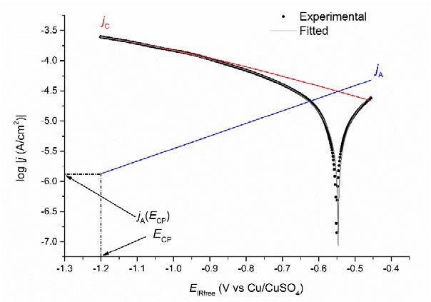
Materials 2021, 14, 4123                                                                                            3 of 22

                           2. Materials and Methods
                           2.1. Preparation of Steel Coupons
                                This study made use of carbon steel S235JR as the testing material because it is com-
                           monly used for gas pipeline transportation system [28]. The nominal chemical composition
                           of this material is (in wt.%): C: 0.17% max., Mn: 1.40% max., P: 0.035% max., Cu: 0.55%
                           max, N: 0.012% max., and Fe for the rest. Cylindrical coupons of diameter 30 mm and 2 mm
                           thickness were cut from the same carbon steel rod. The cut carbon steel coupons were
                           connected to a copper wire and embedded in resin. The carbon steel coupons were me-
                           chanically prepared through grinding at 80 to 600 grits (grain size 26 µm). After grinding,
                           the coupons were rinsed thoroughly with Milli-Q water and dried rapidly with a hairdryer.
                           Only one circular side of the coupon (corresponding to the surface area of 7.07 cm2 ) was
                           exposed to the soil environment.

                           2.2. Soil Preparation and Electrochemical Cell Set Up
                                This study made use of an artificial soil composed of 83 wt.% fine sand (SiO2 ) particles
                           (average particle size 22 µm), 14.5 wt.% clay (kaolinite) and 2.5 wt.% peat. The soil
                           environment used for all the experiments was prepared by incorporating and mixing the
                           electrolyte solution and the artificial soil to achieve ~65% soil saturation level (65% sat.).
                           The selection of the electrolyte shown in Table 1 was mainly based on trying to achieve
                           the solution with species commonly present in soil, particularly Ca2+ and Mg2+, which
                           may play a role during cathodic protection, e.g., by inducing the formation of a calcareous
                           deposit. The resulting pH, once soil and electrolyte were mixed, was measured at 7.1 ± 0.1.
                           All experiments were performed at room temperature (21 ± 2 ◦ C).

                           Table 1. Chemical composition of the electrolyte solution.

                             Compound            NaCl          CaCl2 2H2 O    MgCl 6H2 O     NaSO4 7H2 O      NaHCO3
                             Conc. (g/L)        0.5844           0.2940            0.2033       0.4022          0.1680

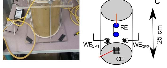
                                  A 19 cm × 25 cm Plexiglas cell (Figure 1) was used to bury two coupons inside the
                           prepared soil, ensuring that they were as far apart from each other as possible. The soil
                           was filled up to about 5–6 cm below the top of the cell to allow the remaining space for air
                           (i.e., O2 ) into the system. The cell was closed with a lid to maintain constant soil moisture.
                           The prepared steel coupons were used as working electrodes. The reference electrode was
                           the Celco 5 (COREXCO, Décines Charpieu, France) copper-copper sulfate (Cu/CuSO4 )
                           electrode (+0.316 V/SHE at 25 ◦ C) specifically designed for soil experiments and commonly
                           used in the field. It was also used in previous studies [10,11,23–27]. All electrochemical
                           potentials were expressed with reference to this electrode, i.e., V vs. Cu/CuSO4 . A titanium
                           grid, placed approximately at the center of the cell, was used as a counter electrode. Soil
                           moisture was controlled during the experiment with a Waterscout SM100 sensor (Spectrum
                           Technologies Inc., Aurora, IL, USA). It proved constant at 63 ± 3% sat.
                                  The two carbon steel coupons, denoted as WECP1 and WECP2 , were buried in soil for
                           90 days. They were left at OCP for the first 7 days of the experiment. This duration was
                           assumed sufficient for the system to reach a steady state, and the corrosion rate was then
                           estimated by electrochemical measurements at day 7. CP was subsequently applied on the
                           coupons for the remaining 83 days of the experiment.
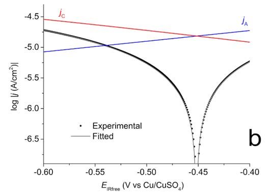
Study of Overprotective-Polarization of Steel Subjected to Cathodic Protection in Unsaturated Soil - MDPI
Materials
Materials 2021,
          2021, 14,
                14, x4123
                      FOR PEER REVIEW                                                                                                         4 4of
                                                                                                                                                  of 22
                                                                                                                                                     22

                                  Figure 1.
                                 Figure       Representationof
                                           1. Representation     of electrochemical
                                                                    electrochemicalcellcellfor
                                                                                            for corrosion
                                                                                                 corrosionstudies
                                                                                                           studiesininsoil:
                                                                                                                       soil: (a)
                                                                                                                              (a)picture
                                                                                                                                  pictureof
                                                                                                                                          of the
                                                                                                                                              the cell,
                                                                                                                                                  cell,
                                  (b) schematic
                                 (b)  schematic top
                                                  top view
                                                      view andand (c)
                                                                   (c) schematic
                                                                        schematic side
                                                                                   side view.
                                                                                        view. CECE ==counter
                                                                                                      counterelectrode,
                                                                                                              electrode,RERE==reference
                                                                                                                                 referenceelectrode,
                                                                                                                                           electrode,
                                  WECP1
                                 WE    CP1==working
                                              workingelectrode
                                                       electrodecathodic
                                                                     cathodicprotection
                                                                                protection 11 (steel
                                                                                              (steel coupon 1) and WEWECP2CP2 == working
                                                                                                                                  working electrode
                                                                                                                                           electrode
                                 cathodic
                                  cathodic protection
                                             protection 22 (steel
                                                           (steel coupon
                                                                  coupon 2).2). The
                                                                                Themoisture
                                                                                     moisture sensor
                                                                                                sensor was
                                                                                                        was omitted
                                                                                                            omitted for
                                                                                                                     for clarity;
                                                                                                                         clarity; the
                                                                                                                                   the sensor
                                                                                                                                       sensor reader
                                                                                                                                               reader
                                 is visible  on the left of  the picture.
                                  is visible on the left of the picture.

                                 2.3. Electrochemistry
                                 2.3. Electrochemistry
                                 2.3.1. Cathodic Protection
                                 2.3.1. Cathodic  Protection
                                       Afterthe
                                       After  thefirst
                                                   first7 7days
                                                            daysat at OCP,
                                                                   OCP,  CPCP
                                                                            waswas applied
                                                                                applied      on coupons
                                                                                         on coupons       WE
                                                                                                      WECP1 and   and
                                                                                                              CP1WE     WECP2 at
                                                                                                                     CP2 at poten‐
                                 potential   values,   corrected    from ohmic drop,  E    =  − 1.0 and − 1.2 V  vs.  Cu/CuSO
                                 tial values, corrected from ohmic drop, ECP = −1.0 and −1.2 V vs. Cu/CuSO4, respectively.4,
                                                                                        CP
                                  respectively. EIS measurements (see next section) were performed at 24-h time intervals to
                                 EIS measurements (see next section) were performed at 24‐h time intervals to determine
                                  determine the soil electrolyte resistance Rs . The applied potential was then corrected from
                                 the soil electrolyte resistance Rs. The applied     potential was then corrected from ohmic
                                  ohmic drop according to the expression:
                                 drop according to the expression:
                                                                          EECP             = E − R ·I
                                                                             CP = EIRfree  Eon  Rs  I
                                                                                =E                                                                (3)
                                                                                                                                                  (3)
                                                                                    IRfree    on   s

                                 where E
                                 where   EIRfree
                                          IRfreeisisthe
                                                      thecorrected   potential,EEononisisthe
                                                           correctedpotential,            theapplied  potential, RRssisisthe
                                                                                              appliedpotential,           thesoil
                                                                                                                              soilelectrolyte
                                                                                                                                  electrolyte
                                  resistance  and   I  is the current flowing through      the electrode. Because
                                 resistance and I is the current flowing through the electrode. Because I may vary   I  may  vary  with with
                                                                                                                                        time,
                                 E     may  also   vary    until another correction     is made  (next
                                   CP ECP may also vary until another correction is made (next day).
                                 time,                                                                 day).

                                  2.3.2. Electrochemical Impedance Spectroscopy (EIS) Experiments
                                 2.3.2. Electrochemical Impedance Spectroscopy (EIS) Experiments
                                        All electrochemical measurements were performed in the cell displayed in Figure 1
                                       All electrochemical measurements were performed in the cell displayed in Figure 1
                                  using Gamry Interface 1000 potentiostats (Gamry Instruments, Warminster, PA, USA)
                                 using Gamry Interface 1000 potentiostats (Gamry Instruments, Warminster, PA, USA)
                                  monitored by the Framework software (V4.35, Gamry Instruments, Warminster, PA, USA).
                                 monitored
                                 The resultsby     the Framework
                                                 obtained              software
                                                             were analyzed        (V4.35,
                                                                               with         GamryEchem
                                                                                     the Gamry       Instruments,
                                                                                                             AnalystWarminster,    PA,
                                                                                                                      software (V6.31,
                                 USA).    The   results  obtained    were  analyzed    with   the  Gamry    Echem
                                  Gamry Instruments, Warminster, PA, USA). Electrochemical impedance spectroscopy    Analyst  software
                                 (V6.31,   Gamry Instruments,
                                 (EIS) measurements                 Warminster,
                                                           were performed     at aPA,  USA). Electrochemical
                                                                                   frequency    between 100 kHz  impedance   spectros‐
                                                                                                                    and 200 mHz,   and
                                 copy   (EIS) measurements       were performed     at a frequency   between   100 kHz
                                  the AC voltage perturbation amplitude (peak to peak) was 0.03 V around the applied     and 200 mHz,
                                 and  the ACpotential
                                 protection     voltage perturbation
                                                          of the sample amplitude    (peak
                                                                          (for coupons       to peak)
                                                                                           under  CP) was   0.03 V OCP
                                                                                                       or around   around  the applied
                                                                                                                        (before the CP
                                 protection   potential   of  the sample  (for coupons    under  CP)   or around  OCP
                                 was applied). This high amplitude was required because of the important ohmic drop     (before thedue
                                                                                                                                    CP
                                 was   applied).  This  high   amplitude  was  required    because  of the important  ohmic  drop
                                  to soil resistivity. The linearity of the system was checked in varying the amplitude of the     due
                                 to
                                 AC soil resistivity.
                                      signal  appliedThe    linearity
                                                        to the        of the system was checked in varying the amplitude of the
                                                                sample.
                                 AC signal applied to the sample.
Study of Overprotective-Polarization of Steel Subjected to Cathodic Protection in Unsaturated Soil - MDPI
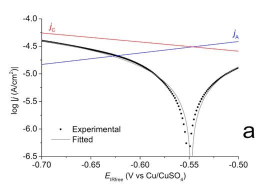
Materials 2021, 14, 4123                                                                                              5 of 22

                                The soil electrolyte resistance Rs can be determined by EIS. It corresponds to the real
                           part of the impedance when the frequency tends towards infinite. It must be noted that Rs
                           is mainly linked, in unsaturated soils, to the “wet” area of the electrode [10,11,25,26], i.e.,
                           the area really in contact with the electrolyte present in the pores of the soil. More precisely,
                           Rs varies inversely to the wet area and, for instance, if the soil dries, i.e., the amount of
                           electrolyte present in the pores decreases, then the wet area decreases and Rs increases. The
                           value of Rs can then indicate if soil moisture varies at the vicinity of the coupon [11].
                                Actually, important variations of Rs were observed between day 7 (beginning of CP)
                           and day 42. This rather corresponds to a transition period between steady state OCP
                           conditions and steady state CP conditions (this is discussed in Section 3.1). For this reason,
                           it was decided to focus the present work on the characterization of the system after day 42.

                           2.3.3. Voltammetry Experiments
                                 For the coupons at OCP during the 7 first days, the polarization curves were recorded
                           at a scan rate (dE/dt) of 0.2 mV/s from OCP up to +0.08 V and down to −0.08 V, i.e.,
                           on a limited range of potential so that the steel surface was only moderately affected.
                           This method was used previously and referred to as “VAOCP” for “voltammetry around
                           OCP” [10,29]. It implies that the voltammograms obtained are mathematically modeled
                           using electrochemical kinetic laws, which was achieved using the OriginPro 2016 Software
                           (SR0 b9.3.226, OriginLab Corporation, Northampton, MA, USA). Electrochemical param-
                           eters such as anodic and cathodic Tafel coefficients are then obtained together with the
                           corrosion current density jcorr . The corrosion rate τ corr is then computed from jcorr using
                           Faraday’s law.
                                 For coupons under CP, the polarization curves were recorded from the applied poten-
                           tial ECP up to (approximately) OCP + 0.08 V, with dE/dt = 0.2 mV/s. They were modelled
                           as described elsewhere [25,26,29], and as also detailed further in the text (Section 3.2), to
                           estimate τ rc , the “residual” corrosion rate. τ rc is actually the corrosion rate associated with
                           the anodic current density jA at the applied potential ECP [23–26], i.e., jA (ECP ). Because
                           voltammetry may affect significantly the behavior of the system, the first polarization
                           curves were acquired at day 42, and only once a week afterwards, except at day 56, i.e., at
                           days 49, 63, 70, 77, 84 and 90. During the first 35 days of CP (from day 7 to day 42), i.e.,
                           during the transition period, the system was thus only subjected to minor perturbations,
                           corresponding to EIS measurements.

                           2.4. µ-Raman Spectroscopy
                                At the end of the experiment, the coupons were removed from the electrochemical
                           cell with a part of soil covering their surface and kept inside a freezer where they were
                           maintained at −24 ◦ C. This experimental procedure was used in previous works and
                           proved adequate to preserve the system from further corrosion and evolution [30,31].
                                µ-Raman spectroscopy analysis was performed at room temperature with a Jobin
                           Yvon High Resolution Raman Spectrometer (LabRAM HR, Horiba, Tokyo, Japan) equipped
                           with a microscope (Olympus BX 41, Olympus, Tokyo, Japan), a Peltier-based cooled charge
                           coupled detector (CCD) and a He-Ne laser (632.8 nm). The laser power was kept at
                           10% of the maximum (i.e., 0.9 mW) to prevent an excessive heating that can induce the
                           transformation of the analyzed compounds into hematite (α-Fe2 O3 ). The acquisition time
                           was variable but equal to 60 s in most cases. It could be increased up to 5 min to optimize
                           the signal to noise ratio. At least 20 zones (diameter of ~6 µm) of each sample were
                           analyzed through a 50× objective, with a resolution of 0.1 cm−1 .

                           3. Results
                           3.1. Electrochemical Impedance Spectroscopy
                                 EIS measurements were performed on both coupons at various exposure times in
                           soil at OCP or under CP. In the present case dealing with a resistive medium, a parasitic
                           influence of the reference electrode at high frequency was observed [32], and Rs was then
soil during the whole experiment. During the OCP period (days 1–7), Rs increases from
                           1670 to 1865 Ω cm2 for coupon WECP1 and from 1380 to 1815 Ω cm2 for coupon WECP2. This
                           increase in Rs can be attributed to the changes in soil physicochemical properties. Actually,
                           water tends to flow vertically in the cell, because of gravity, so that a gradient of soil mois‐
Materials 2021, 14, 4123   ture appears with time. This movement of fluid necessarily modifies the soil at the vicinity               6 of 22
                           of the coupons during the first days. Moreover, corrosion products are formed on the
                           metal surface, which also modifies the steel/soil interface.
                                 The application of CP leads to an immediate sharp increase in Rs to ~2250 Ω cm2 for
                           determined
                           coupon     WECP1at 10andkHz,
                                                      ~3850i.e.,ΩRcm
                                                                   s =2 Re(Z) at 10 kHz.
                                                                        for coupon    WECP2 For the same
                                                                                             . Various      reasonoccur
                                                                                                        changes    the EIS
                                                                                                                         at data  obtained
                                                                                                                            the steel/elec‐
                           at frequencies
                           trolyte   interface  higher
                                                   whenthan  CP10 is kHz   weredissolved
                                                                     applied:    not considered
                                                                                              O2 is and  are not and
                                                                                                     consumed     shown    on the Nyquist
                                                                                                                       interfacial   pH in‐
                           plots   except   when      noted.
                           creases, the electric field induces migration of ions, electrocapillary effects modify the con‐
                                 First,between
                           tact angle    Figure 2 liquid
                                                       displays    the and
                                                                phase   evolution
                                                                             metal,of  RsItwith
                                                                                     etc.        timenoticing
                                                                                            is worth   for coupons    WECP1
                                                                                                                that there  is aand  WECP2
                                                                                                                                 difference
                           in soil  during     the  whole     experiment.     During   the  OCP   period
                           of 1600 Ω cm in Rs values obtained between coupons WECP1 and WECP2 after
                                             2                                                             (days 1–7),  Rs increases
                                                                                                                              8 days.from
                                                                                                                                       This
                                         canΩthen                                                             Ω cm
                           1670 to 1865          cm be2 forattributed
                                                             coupon WE           and fromapplied
                                                                                              1380 toE1815          2
                           difference                                    to the
                                                                             CP1 different             CP values  setfor
                                                                                                                      for coupon
                                                                                                                          couponsWE       CP1.
                                                                                                                                      WECP2
                           ThisWE
                           and    increase     in Rs can
                                      CP2, i.e., −1.0   andbe     attributed
                                                               −1.2            to the changes
                                                                     V vs. Cu/CuSO                 in soil physicochemical properties.
                                                                                        4, respectively. This indicates that lower ECP
                           Actually,
                           leads       water R
                                   to higher     tends    to flow vertically in the cell, because of gravity, so that a gradient of
                                                   s. This initial increase of Rs is, however, followed by a rapid decrease so
                           soil moisture      appears
                           that at day 14 both Rs values   with time.     This movement
                                                                    are similar               of fluid necessarily
                                                                                  to those measured     at OCP. This  modifies   the soil at
                                                                                                                        initial increase   of
                           the  vicinity   of  the   coupons     during    the first days.  Moreover,   corrosion   products
                           Rs is then a transient phenomenon that was not further studied and is yet to be explained.           are formed
                           on the metal surface, which also modifies the steel/soil interface.

                           Figure 2.
                           Figure    Rssevolution
                                  2. R   evolutionwith
                                                  withexposure
                                                       exposuretime
                                                                timefor
                                                                     forcoupons
                                                                         couponsWE
                                                                                WECP1  andWE
                                                                                   CP1and  WE   . .
                                                                                               CP2
                                                                                             CP2

                                The application of CP leads to an immediate sharp increase in Rs to ~2250 Ω cm2
                                However, clear trends are observed      after day 21. For coupon WECP1, Rs decreases fur‐
                           for coupon WECP1 and ~3850 Ω cm2 for coupon WECP22. Various changes occur at the
                           ther before reaching    a constant value of 890 ± 50 Ω cm after day 42, indicating that a
                           steel/electrolyte interface when CP is applied: dissolved O2 is consumed and interfacial
                           pH increases, the electric field induces migration of ions, electrocapillary effects modify
                           the contact angle between liquid phase and metal, etc. It is worth noticing that there is
                           a difference of 1600 Ω cm2 in Rs values obtained between coupons WECP1 and WECP2
                           after 8 days. This difference can then be attributed to the different applied ECP values set
                           for coupons WECP1 and WECP2 , i.e., −1.0 and −1.2 V vs. Cu/CuSO4, respectively. This
                           indicates that lower ECP leads to higher Rs . This initial increase of Rs is, however, followed
                           by a rapid decrease so that at day 14 both Rs values are similar to those measured at OCP.
                           This initial increase of Rs is then a transient phenomenon that was not further studied and
                           is yet to be explained.
                                However, clear trends are observed after day 21. For coupon WECP1 , Rs decreases
                           further before reaching a constant value of 890 ± 50 Ω cm2 after day 42, indicating that
                           a steady state has been reached. This value is actually ~800 Ω cm2 lower than the initial
                           value of 1670 Ω cm2 (day 3). This result is consistent with previous study [25], where the
                           decrease of Rs was attributed to an increase of the “wet area” due to electrocapillary effects.
                           A negative shift of potential allows the liquid phase to spread over the steel surface because
                           it decreases the solid–liquid contact angle θ [33–36].
steady state has been reached. This value is actually ~800 Ω cm2 lower than the initial
                           value of 1670 Ω cm2 (day 3). This result is consistent with previous study [25], where the
                           decrease of Rs was attributed to an increase of the “wet area” due to electrocapillary ef‐
Materials 2021, 14, 4123                                                                                                                                 7 of 22
                           fects. A negative shift of potential allows the liquid phase to spread over the steel surface
                           because it decreases the solid–liquid contact angle θ [33–36].
                                  In contrast, Rs values obtained for coupon WECP2 after 21 days take an opposite trend
                           in relation     to that observed
                                   In contrast,       Rs valuesfor         coupon for
                                                                       obtained       WEcoupon
                                                                                            CP1, i.e., increase
                                                                                                        WECP2 afteragain21   with
                                                                                                                               daysexposure
                                                                                                                                       take antime.      This
                                                                                                                                                   opposite
                           increase
                            trend inisrelation
                                           not continuous,         and somefor
                                                      to that observed              fluctuations
                                                                                       coupon WE      areCP1observed,      with local
                                                                                                             , i.e., increase    againminima          at days
                                                                                                                                           with exposure
                           42  and This
                            time.     70. Rincrease
                                             s reaches is  a final      value of ~2400
                                                              not continuous,             andΩsome cm2 after    90 days, are
                                                                                                          fluctuations       thusobserved,
                                                                                                                                    being ~1000  with  Ω local
                                                                                                                                                           cm2
                           higher
                            minima    than    the initial
                                         at days     42 andvalue70. Rof       1380 Ωacm
                                                                           s reaches        final(day
                                                                                               2
                                                                                                    value3).ofAt~2400
                                                                                                                   the CP Ω cm    2
                                                                                                                              potential
                                                                                                                                     after of
                                                                                                                                            90 −1.2
                                                                                                                                                 days,Vthus vs.
                           Cu/CuSO
                            being ~1000       Ω cathodic
                                         4, the   cm2 higher   process
                                                                    than the  is enhanced,
                                                                                  initial value     of 1380toΩthe
                                                                                                  leading              2 (day 3). At of
                                                                                                                   cmacceleration        theOCP2 consump‐
                                                                                                                                                    potential
                           tion
                            of −at 1.2the   steel/electrolyte
                                         V vs.   Cu/CuSO4 , the       interface
                                                                            cathodic andprocess
                                                                                           more likely       to the increase
                                                                                                      is enhanced,       leadingof   towater     reduction
                                                                                                                                         the acceleration
                           rate.
                            of OThe      increase of R
                                   2 consumption          ats with      time may then be
                                                              the steel/electrolyte                due to the
                                                                                                 interface    andaccumulation
                                                                                                                     more likely to   of the
                                                                                                                                           hydrogen
                                                                                                                                                increase  (Hof2)

                           bubbles      that formrate.
                            water reduction           on theThesteel      surface
                                                                    increase      ofaccording
                                                                                      Rs with time  to Equation
                                                                                                          may then    (2).
                                                                                                                        beThis
                                                                                                                             duephenomenon
                                                                                                                                   to the accumulation would
                           indeed     lead to(H
                            of hydrogen          a 2decrease
                                                     ) bubblesofthat   the “wet”
                                                                             form on  areathe(i.e.,
                                                                                                steelthe  area inaccording
                                                                                                       surface       contact with      the liquid(2).
                                                                                                                                 to Equation           phase)
                                                                                                                                                          This
                            phenomenon
                           and   thus to an wouldapparent  indeed
                                                               increase  leadoftoRas [10,25].
                                                                                      decrease       of cathodic
                                                                                                   The  the “wet”processes
                                                                                                                       area (i.e.,taking
                                                                                                                                     the area     in contact
                                                                                                                                              place    at −1.2
                           Vwith   the liquid 4phase)
                              vs. Cu/CuSO                   and thus
                                                   are studied         andtodiscussed
                                                                               an apparent                   of Rs [10,25]. The cathodic processes
                                                                                                  increase3.2.
                                                                                             in Section
                            taking    place    at −
                                  The Nyquist EIS plots obtained4for both couponsdiscussed
                                                     1.2  V   vs.  Cu/CuSO            are   studied     and     before the   in application
                                                                                                                                Section 3.2. of CP are
                           comparedThe Nyquist
                                           in FigureEIS   3. plots      obtaineddiagrams
                                                              Both Nyquist            for both coupons           before features,
                                                                                                    display similar         the application
                                                                                                                                        thoughof       CP are
                                                                                                                                                    they    are
                            compared
                           more     clearlyinseen
                                                Figurefor 3.  Both Nyquist
                                                           coupon         WECP2. Adiagrams           displayloop
                                                                                        first capacitive        similar     features,
                                                                                                                      is present         though
                                                                                                                                     at high         they are
                                                                                                                                                frequency,
                            more clearly
                           followed      by aseen
                                                linear forpart
                                                            coupon
                                                                 and aWE        CP2 . Acapacitive
                                                                             second       first capacitive
                                                                                                        loop at loop
                                                                                                                   lowisfrequency.
                                                                                                                            present at Thehighlinear
                                                                                                                                                 frequency,
                                                                                                                                                          part
                            followed
                           makes     anglesby aoflinear
                                                    45° andpart50°and      a second
                                                                        with    Re(Z) capacitive
                                                                                         for coupons     loop
                                                                                                            WEat CP1low
                                                                                                                      andfrequency.        The linearThis
                                                                                                                             WECP2, respectively.          part
                            makes     angles    of  45  ◦ and 50◦ with Re(Z) for coupons WE                           and    WE        respectively.      This
                           shows the influence of a diffusional process. Previous studies                       CP1      reportedCP2, that the cathodic
                            shows the
                           reaction         influence
                                        of the            of a diffusional
                                                 steel buried        in unsaturated process. soilPrevious
                                                                                                   was indeed  studies     reported
                                                                                                                    partially           that the
                                                                                                                                controlled      bycathodic
                                                                                                                                                      the dif‐
                           fusion of O2 [10,24]. Actually, the obtained Nyquist diagrams are characteristicbyofthe
                            reaction      of the   steel   buried        in  unsaturated         soil  was    indeed     partially    controlled              a
                            diffusiondiffusion
                           bounded         of O2 [10,24].       Actually,i.e.,
                                                        phenomenon,              the aobtained       Nyquist
                                                                                         finite‐length            diagrams
                                                                                                            diffusion      for aare   characteristic
                                                                                                                                  planar     electrode.of   Ata
                            bounded
                           the  beginning diffusion
                                                of thephenomenon,
                                                         corrosion process,    i.e., athe
                                                                                       finite-length
                                                                                            corrosiondiffusion         for a is
                                                                                                           product layer       planar
                                                                                                                                 very electrode.
                                                                                                                                         thin and shouldAt the
                            beginning       of the   corrosion      process,      the  corrosion      product     layer
                           not hinder the diffusion of O2. The O2 concentration gradient is then located in the soil      is very   thin   and   should     not
                            hinder     the  diffusion     of  O  2 .
                           itself, as observed in previous work [37]. The    O  2 concentration        gradient     is then   located     in the   soil  itself,
                            as observed in previous work [37].

                                       EISNyquist
                            Figure3.3.EIS
                           Figure         NyquistatatOCP
                                                     OCP(day
                                                         (day7)7)for
                                                                  forcoupons
                                                                      couponsWE
                                                                             WECP1  andWE
                                                                                CP1and  WE   . .
                                                                                            CP2
                                                                                          CP2

                                 The EIS data at OCP were then modelled using the electrical equivalent circuit (EEC)
                            displayed in Figure 4a. In this EEC, Rs is the soil electrolyte resistance, Rt is the charge
                            transfer resistance, Qdl a constant phase element (CPE) used to represent the double layer
                            capacitance and W d is a bounded diffusion impedance. The CPE was used instead of an
                            ideal capacitance because the first attempts to model the experimental data, performed with
                            a capacitance, did not lead to acceptable goodness-of-fit. Actually, CPE is commonly used
The EIS data at OCP were then modelled using the electrical equivalent circuit
                                                     displayed in Figure 4a. In this EEC, Rs is the soil electrolyte resistance, Rt is the c
                                                     transfer resistance, Qdl a constant phase element (CPE) used to represent the double
 Materials 2021, 14, 4123                            capacitance and Wd is a bounded diffusion impedance. The CPE was8used      of 22 instead
                                                     ideal capacitance because the first attempts to model the experimental data, perfo
                                                     with a capacitance, did not lead to acceptable goodness‐of‐fit. Actually, CPE is comm
                                                     used because it takes into account various effects due to inhomogeneity, porosity, r
                                      because it takes into account various effects due to inhomogeneity, porosity, roughness
                                                     ness and other non‐ideal dielectric properties of the electrode [38]. The results obt
                                      and other non-ideal dielectric properties of the electrode [38]. The results obtained via this
                                                     via this modelling are discussed together with those obtained for the coupons und
                                      modelling are discussed together with those obtained for the coupons under CP at the end
                                                     at the end of this section.
                                      of this section.

                                        Figure
                                      Figure    4. EEC
                                             4. EEC    used
                                                     used    to fit
                                                          to fit thethe
                                                                     EISEIS data
                                                                         data    obtained
                                                                              obtained    at OCP
                                                                                       at OCP  (a) (a) or under
                                                                                                    or under CPCP
                                                                                                                (b)(b)
                                                                                                                    forfor both
                                                                                                                        both    coupons.
                                                                                                                             coupons.

                                          The influenceThe  of CP    can be of
                                                                  influence     observed
                                                                                   CP can beon observed
                                                                                                 the Nyquist     plots
                                                                                                            on the      of Figures
                                                                                                                     Nyquist     plots5ofand    6. As5 and 6. A
                                                                                                                                            Figures
                                    explained in Section      2.3.2, only    the data  obtained    after day  42 are  discussed.    These
                                                     plained in Section 2.3.2, only the data obtained after day 42 are discussed. These Ny   Nyquist
                                    diagrams consistently
                                                     diagramsexhibit         a flattened
                                                                   consistently           semi-circle
                                                                                    exhibit  a flattened loop,  followedloop,
                                                                                                            semi‐circle       by what
                                                                                                                                  followedmay bybe an
                                                                                                                                                    what may
                                    incomplete second       loop atsecond
                                                     incomplete        lower frequency.
                                                                                loop at lowerThefrequency.
                                                                                                   main flattened
                                                                                                              The mainsemi-circle
                                                                                                                           flattenedloop    is charac-loop is ch
                                                                                                                                        semi‐circle
                                    terized, like that   observed
                                                     terized,           at OCP,
                                                                like that         by a linear
                                                                              observed   at OCP,behavior    at high
                                                                                                    by a linear       frequency.
                                                                                                                  behavior           However,
                                                                                                                               at high   frequency.the Howeve
                                    initial linear part  of  the  Nyquist      diagrams   obtained    under   CP   after day   42  makes
                                                     initial linear part of the Nyquist diagrams obtained under CP after day 42 makes an     an  angle
                                    of 30◦ and 25◦ofwith      Re(Z)
                                                        30° and     25°for  coupons
                                                                         with   Re(Z) WE   CP1 and WE
                                                                                       for coupons     WECP2,   respectively, as illustrated on
                                                                                                           CP1 and WECP2, respectively, as illustrated o
                                    day 42 Nyquist      plot   in  Figure    5 and   day  63 Nyquist
                                                     42 Nyquist plot in Figure 5 and day 63 Nyquist      plot in  Figure
                                                                                                                      plot 6.
                                                                                                                            in This
                                                                                                                                Figuresuggests
                                                                                                                                          6. Thisthat
                                                                                                                                                   suggests th
                                    the steel coupons      behave     as   semi-infinite   porous     conductive     electrodes
                                                     steel coupons behave as semi‐infinite porous conductive electrodes [37,39,40].[37,39,40].    The        Th
                                    cathodic process,    predominant        under   CP,  would    then  involve   the  diffusion   of
                                                     thodic process, predominant under CP, would then involve the diffusion of O2 insidO 2 inside  the
                                    pores of a conductive
                                                     pores ofmineral       film covering
                                                                 a conductive       mineralthe   steel
                                                                                              film     surface the
                                                                                                     covering   andsteel
                                                                                                                      its reduction
                                                                                                                            surface andall along   the
                                                                                                                                             its reduction  all
                                    conductive walls of the pores. At OCP, the initial linear part of the Nyquist diagram made
                                                     the conductive        walls   of the pores.   At  OCP,   the  initial  linear  part   of  the Nyquist  dia
                                    an angle of about 45◦ with the Re(Z) axis (Figure 3). The impedance, mainly corresponding
                                                     made an angle of about 45° with the Re(Z) axis (Figure 3). The impedance, mainly
                                    to a bounded diffusion impedance, then described the diffusion rate of oxygen through a
                                                     sponding to a bounded diffusion impedance, then described the diffusion rate of ox
Materials 2021, 14, x FOR PEER REVIEW
                                    non-conducting porous layer, which in the present case was more likely the soil itself.                   9 of 22
                                                                                                                                                    At
                                                     through a non‐conducting porous layer, which in the present case was more likely th
                                    day 42, i.e., after 35 days under CP, the impedance describes the diffusion (and reduction)
                                                     itself. At day 42, i.e., after 35 days under CP, the impedance describes the diffusion
                                    of O2 in the pores of a conductive layer that formed later under CP.
                                                     reduction) of O2 in the pores of a conductive layer that formed later under CP.
                                                           Furthermore, the influence of the applied potential is also clearly revealed. In th
                                                     of the CP potential of −1.0 V vs. Cu/CuSO4, i.e., coupon WECP1 as shown in Figure
                                                     flattened semi‐capacitive loop at high frequency of the Nyquist plots is observed
                                                     crease in magnitude with exposure time. In the present case, the electrochemical pr
                                                     is mainly controlled by the diffusion of O2 inside the pores of the mineral film cov
                                                     the steel surface. Consequently, the gradual increase of the resistance associated wit
                                                     electrochemical process indicates that the mineral film hinders more and more effic
                                                     the diffusion of O2.
                                                           In the case of excessive CP, i.e., coupon WECP2 as shown in Figure 6, the evolut
                                                     the Nyquist plots with exposure time is significantly different. The main difference r
                                                     to the evolution of Rs, whose value increases with time in this case (see also Figure 2
                                                     diameter of the main flattened loop increases with time between day 42 and day
                                                     observed for coupon WECP1, but does not seem to increase afterwards.

                                                Evolutionofofthe
                                     Figure5.5.Evolution
                                    Figure                     theEIS
                                                                   EISNyquist
                                                                       Nyquistplots
                                                                               plotswith
                                                                                    with exposure
                                                                                         exposure time
                                                                                                  time for
                                                                                                       for coupon
                                                                                                           coupon WE
                                                                                                                  WECP1          −1.0
                                                                                                                          (ECP==−1.0
                                                                                                                     CP1 (ECP        VV
                                                                                                                                      vs.vs.
                                     Cu/CuSO       ) between  days  42
                                    Cu/CuSO4) between days 42 and 90.
                                                 4                     and 90.
Materials 2021, 14, 4123   Figure 5. Evolution of the EIS Nyquist plots with exposure time for coupon WECP1 (ECP = −1.0 V vs.22
                                                                                                                        9 of
                           Cu/CuSO4) between days 42 and 90.

                                        Evolutionofofthe
                            Figure6.6.Evolution
                           Figure                     theEIS
                                                          EISNyquist
                                                              Nyquist plots
                                                                       plots with
                                                                             with exposure
                                                                                  exposure time
                                                                                           time for
                                                                                                for coupon
                                                                                                    coupon WE
                                                                                                           WECP2         −1.2VVvs.
                                                                                                                  (ECP==−1.2
                                                                                                              CP2 (ECP
                                                                                                                                vs.
                            Cu/CuSO
                           Cu/CuSO         ) between
                                      4) 4between    days
                                                   days  4242 and
                                                            and 90.90.

                                   Furthermore,
                                  To              the influence
                                     obtain additional          of theand
                                                         information    applied potential
                                                                           quantify        is also clearly
                                                                                      the evolution   of therevealed.
                                                                                                             steel/soilIn the case
                                                                                                                        interface
                             of the  CP  potential  of − 1.0 V vs. Cu/CuSO
                           with time, a modelling of the EIS data obtained      , i.e., coupon   WE
                                                                               4 for the coupons CP1 under CP was achieved.5,
                                                                                                          as shown   in  Figure
                             the flattened semi-capacitive loop at high frequency of the Nyquist plots is observed to
                           The EEC used for both coupons is displayed in Figure 4b. In this EEC, Q1 and R1 are a CPE
                             increase in magnitude with exposure time. In the present case, the electrochemical process
                           and a resistance, respectively, used to model the phenomenon associated with the main
                             is mainly controlled by the diffusion of O inside the pores of the mineral film covering
                           flattened capacitive loop present in all cases2 (Figures 5 and 6). Q2 and R2 are the elements
                             the steel surface. Consequently, the gradual increase of the resistance associated with this
                           used to fit the low frequency part of the impedance diagram. Because only a very small
                             electrochemical process indicates that the mineral film hinders more and more efficiently
                           part of the corresponding capacitive loop (if one assumes this is really a capacitive loop)
                             the diffusion of O2 .
                           is seen, various values   could be obtained for Q2 and R2 parameters and consequently these
                                   In the case of excessive CP, i.e., coupon WECP2 as shown in Figure 6, the evolution of
                             the Nyquist plots with exposure time is significantly different. The main difference relates
                             to the evolution of Rs , whose value increases with time in this case (see also Figure 2). The
                             diameter of the main flattened loop increases with time between day 42 and day 63, as
                             observed for coupon WECP1 , but does not seem to increase afterwards.
                                   To obtain additional information and quantify the evolution of the steel/soil interface
                            with time, a modelling of the EIS data obtained for the coupons under CP was achieved.
                            The EEC used for both coupons is displayed in Figure 4b. In this EEC, Q1 and R1 are a CPE
                             and a resistance, respectively, used to model the phenomenon associated with the main
                             flattened capacitive loop present in all cases (Figures 5 and 6). Q2 and R2 are the elements
                             used to fit the low frequency part of the impedance diagram. Because only a very small
                            part of the corresponding capacitive loop (if one assumes this is really a capacitive loop) is
                             seen, various values could be obtained for Q2 and R2 parameters and consequently these
                            parameters are not presented nor discussed. Various fits were performed, with different
                            values for R2 and Q2 , to study the influence of these parameters on the values obtained
                             for R1 and Q1 . It was noted that R1 and Q1 were not significantly influenced by R2 and Q2 .
                            The considered EEC led to satisfactory fittings of the experimental data, as illustrated by
                             Figure 7.
                                   Figure 7a shows as an example the Nyquist plot for coupon WECP1 at OCP (day 7)
                             and Table 2 gathers the results obtained for both coupons at OCP. It can be seen that the
                             numerical values are similar for both coupons, except for resistance Rd . In the expression
                             of the bounded diffusion impedance W d , Rd is a scaling factor that depends on the kinetics
                             of the interfacial reaction and the bulk concentration of the electroactive species. The larger
                            value of Rd for coupon WECP2 suggests a lower O2 concentration. This would indicate a
                             faster O2 consumption at the vicinity of coupon WECP2 . This faster evolution may also
larger value of Rd for coupon WECP2 suggests a lower O2 concentration. This would indi‐
                           cate a faster O2 consumption at the vicinity of coupon WECP2. This faster evolution may
                           also correlate with the faster evolution of Rs observed for this coupon between day 1 and
                           day 7 (Figure 2). In conclusion, both coupons behave quite similarly at OCP, as confirmed
                           by voltammetry measurements (Section 3.2).
Materials 2021, 14, 4123                                                                                                       10 of 22
                           Table 2. Fitted values of EIS data for both coupons at OCP (day 7).

                                                                                                                         Qdl
                              Coupon       Rs (Ω cm )      n
                                                                ofRRt (Ω cm )     Rd (Ω cm )      td (s)
                                                       2                        2                2
                           correlate with the  faster evolution       s observed for this coupon between day     1 and
                                                                                                             (F cm −2 sn−1day
                                                                                                                          )
                           7 (Figure
                               WECP12). In conclusion,
                                              1864       both
                                                         0.70 coupons  566behave quite841
                                                                                       similarly at0.39
                                                                                                     OCP, as confirmed
                                                                                                              4.2 × 10⁻⁴ by
                           voltammetry
                               WECP2     measurements
                                              1816        (Section 3.2).
                                                         0.72          455           1818         0.35        2.8 × 10⁻⁴

                                   7. EIS
                           Figure 7.  EIS modelling:
                                          modelling: Nyquist
                                                      Nyquist plots
                                                                plots for
                                                                       for coupon
                                                                           coupon WE
                                                                                   WECP1
                                                                                       CP1 (a)
                                                                                           (a) at
                                                                                               at OCP
                                                                                                  OCP at day 7 and (b)
                                                                                                                    (b) under
                                                                                                                        under CPCP at
                                                                                                                                   at
                           day 70.
                           day 70. Owing
                                    Owingtotoa alower
                                                  lower  s value,
                                                      RsRvalue, thethe
                                                                    datadata obtained
                                                                          obtained     at day
                                                                                   at day      70 were
                                                                                           70 were     usable
                                                                                                   usable from from  100tokHz
                                                                                                               100 kHz     100 to 100
                                                                                                                               mHz.
                           mHz.

                           Table 2. Fitted values of EIS data for both coupons at OCP (day 7).

                                                                                                                        Qdl
                            Coupon       Rs (Ω cm2 )          n       Rt (Ω cm2 )     Rd (Ω cm2 )        td (s)
                                                                                                                   (F cm−2 sn−1 )
                            WECP1            1864           0.70          566              841           0.39        4.2 × 10⁻⁴
                            WECP2            1816           0.72          455             1818           0.35        2.8 × 10⁻⁴

                                Figure 7b shows as an example the Nyquist plot for coupon WECP1 under CP at day
                           70, and Table 3 gathers the results obtained between days 42 and 90 for both coupons.
                           First, as observed qualitatively using the Nyquist plots of Figures 5 and 6, the resistance
                           R1 associated with the main capacitive loop increases continuously with time for coupon
                           WECP1 , to reach a maximum of 1661 Ω cm2 at day 90. For coupon WECP2 , after an initial
                           increase between days 42 and 63, where a maximum of 1334 Ω cm2 is reached, R1 decreases
                           slightly to end at 1230 Ω cm2 .
Materials 2021, 14, 4123                                                                                            11 of 22

                           Table 3. Fitted values of EIS data for coupons WECP1 and WECP2 under CP.

                                                                                                              Q1
                               Coupon         Time (d)       Rs (Ω cm2 )     R1 (Ω cm2 )       n
                                                                                                         (F cm−2 sn−1 )
                               WECP1             42              940            659           0.60        2.8 × 10⁻⁶
                                                 49              898            834           0.59        4.2 × 10⁻⁶
                                                 63              838            1179          0.59        4.5 × 10⁻⁶
                                                 70              834            1255          0.59        4.4 × 10⁻⁶
                                                 77              930            1362          0.59        4.2 × 10⁻⁶
                                                 84              916            1534          0.58        5.3 × 10⁻⁶
                                                 90              926            1661          0.56        6.3 × 10⁻⁶
                               WECP2             42             1711             595          0.53        7.5 × 10⁻⁶
                                                 49             1852             707          0.52        6.4 × 10⁻⁶
                                                 63             2142            1334          0.58        3.1 × 10⁻⁶
                                                 70             2241            1318          0.57        3.6 × 10⁻⁶
                                                 77             2382            1253          0.58        3.5 × 10⁻⁶
                                                 84             2382            1254          0.59        2.8 × 10⁻⁶
                                                 90             2425            1230          0.58        3.2 × 10⁻⁶

                                 It is interesting to note that the n coefficient of the CPE is low, between 0.52 and
                           0.60 considering both coupons. This coefficient measures the deviation from an ideal
                           behavior, i.e., n = 1 for a true capacitor and n < 1 for a CPE. However, a “real” CPE is
                           characterized by n values higher than 0.7, and n = 0.5 corresponds to a diffusion element.
                           The values of n obtained here in each case confirm that the cathodic process, i.e., mainly
                           oxygen reduction, is strongly influenced by diffusion. Parameter R1 can then be considered
                           as a “resistance to diffusion” induced by the mineral layer growing on the steel surface and
                           inside the pores of the soil. For coupon WECP1 , the continuous increase of this resistance
                           shows that this layer is more and more protective as it grows with time. Simultaneously,
                           the CPE element Q1 also increases continuously with time. It was observed that the
                           Nyquist plots corresponded to a porous conductive electrode behavior, more likely due
                           to the formation of a porous magnetite layer [20,27]. The growth of this conductive layer
                           would increase the overall cathodic surface, thus leading to an increase of the associated
                           capacitance.
                                 Moreover, the increase of R1 for coupon WECP1 is not associated with an increase of
                           Rs , which indicates that this increased “resistance to diffusion” is not in any case associated
                           with a decrease in the active area of the electrode. It can really be attributed to the growth
                           of the porous conductive layer that covers the steel surface and progressively hinders more
                           and more the transport of O2 .
                                 In the case of coupon WECP2 , the initial increase of R1 is associated with an increase
                           of Rs that may be due to a decrease of the active area [25]. However, Rs increases from
                           1711 Ω cm2 to 2142 Ω cm2 between day 42 and day 63, i.e., an increase of +25%, while
                           R1 increases from 595 Ω cm2 to 1334 Ω cm2 , i.e., an increase of +124%. Consequently, the
                           main reason for this initial increase of R1 is not the possible decrease of the active area but,
                           as for coupon WECP1 , a real increase of the “resistance to diffusion” associated with the
                           growth of the porous conductive layer. However, R1 decreases slightly after day 63, while
                           Q1 decreases as soon as day 42 and fluctuates after day 63. This shows that the protective
                           ability of the porous conductive layer is influenced by a phenomenon that does not take
                           place for coupon WECP1 . This could be due to the hydrogen evolution reaction that should
                           be more important at the lower potential of −1.2 V vs. Cu/CuSO4 . Hydrogen evolution
                           could damage, through the release of H2 bubbles, the porous conductive layer. This point
                           is discussed further at the end of Section 3.3.

                           3.2. Voltammetry and Estimation of Residual Corrosion Rate
                                The voltammograms obtained in this study were computer fitted using theoretical
                           kinetic laws. From the EIS experiments, discussed in the previous section, it was observed
Materials 2021, 14, 4123                                                                                                                                 12 of 22

                                 that the cathodic process, mainly linked to O2 reduction, was at least partially controlled
                                 by diffusion. Therefore, the mathematical modelling of the voltammograms j(E) used in
                                 the present study, adapted from that reported previously [10,11,25,27], was described by
                                 the following expression:

                                                                                                                 1
                                                j = j A + jC = jcorr ·e β A (E− Ecorr ) +                                                                    (4)
                                                                                             1                                 1           1
                                                                                            jlim   − e− βC (E−Ecorr ) ·       jcorr   +   jlim

                                    where j = overall current density, jA = anodic current density, jC = cathodic current den-
                                    sity, jcorr = corrosion current density, jlim = limiting current density (O2 diffusion) in
                                    A/cm2 , Ecorr = corrosion potential in V vs. Cu/CuSO4 , βA = anodic Tafel coefficient and
                                    βC = cathodic Tafel coefficient for O2 reduction in V−1 .
                                          This model corresponds to an anodic process controlled by charge transfer and a ca-
                                    thodic process partially controlled by diffusion (mixed control) [10,24,25,29]. The cathodic
                                    process is then in this case restricted to O2 reduction. An additional contribution due to
                                    water reduction was envisioned. However, this model implied a very large number of
                                    adjustable parameters and the procedure proved unreliable as various solutions could be
                                    obtained for the fitting of the experimental curves. It was consequently discarded.
                                          Equation (4) was then used in any case to perform the mathematical modelling,
                                    and Figure 8 shows as an example the computer fitted log|j| vs. E voltammogram
                                    obtained after 49 days for coupon WECP1 . In any case, the quality of the fitting proved
                                    excellent, which demonstrates that the electrochemical model was adequate. Actually,
                                    at ECP = −1.0 V vs. Cu/CuSO4 , it was indeed expected that the contribution of water
                                    reduction was negligible. The current density jA (ECP ) was extrapolated from the13anodic
Materials 2021, 14, x FOR PEER REVIEW                                                                                          of 22
                                    Tafel line log|jA | vs. E, as illustrated in Figure 8. From the extrapolated jA (ECP ) value, the
                                    residual corrosion rate τ rc was estimated via Faraday’s law.

                                            Polarizationcurves
                                 Figure8.8.Polarization
                                Figure                     curvesfor
                                                                  forcoupon
                                                                      couponWE WECP1CP1atatday
                                                                                            day49:
                                                                                                 49:experimental‐curve
                                                                                                      experimental-curve(black
                                                                                                                          (blackdots),
                                                                                                                                 dots),fitted‐
                                                                                                                                         fitted-
                                curve
                                 curve(grey
                                        (grey full
                                              full line), anodic
                                                          anodic(blue
                                                                 (blueline)
                                                                        line)and
                                                                              andcathodic
                                                                                   cathodic    (red
                                                                                            (red     line)
                                                                                                  line)    components
                                                                                                        components    drawn
                                                                                                                   drawn       using
                                                                                                                           using     the ob‐
                                                                                                                                 the obtained
                                tained electrochemical
                                 electrochemical           parameters.
                                                    parameters.

     Table 4. Summary of fitted parameters computed from mathematical modelling for coupon WECP1 (CSE = copper/copper
     sulfate electrode).

                   Ecorr/       jcorr/          jA(ECP)/             jlim/           bA/                  bC/                  τcorr/                 τrc/
     Day
                   VCSE        A cm−2            A cm−2            A cm−2           mV/dec               mV/dec               μm yr−1                μm yr−1
   7 (OCP)         −0.85     2.86 × 10⁻⁵            ‐             −1.37 × 10⁻⁴        52                   62                  330                      ‐
      42           −0.54     2.71 × 10⁻⁵       1.62 × 10⁻⁶        −3.06 × 10⁻⁴        380                 290                    ‐                     19
      49           −0.45     1.52 × 10⁻⁵       1.64 × 10⁻⁶        −5.74 × 10⁻⁴        575                 460                    ‐                     19
      63           −0.37     3.01 × 10⁻⁵       1.59 × 10⁻⁶        −5.39 × 10⁻⁴        460                 575                    ‐                     18
                                      −5                 −6                  −4
Materials 2021, 14, 4123                                                                                                    13 of 22

                                      All the fitted parameters for coupon WECP1 are listed in Table 4. To facilitate compar-
                                 ison with published data, the Tafel coefficients βA,C were converted to Tafel slopes bA,C
                                 using the expression:
                                                                                ln(10)
                                                                        b A,C =                                           (5)
                                                                                | β A,C |

      Table 4. Summary of fitted parameters computed from mathematical modelling for coupon WECP1 (CSE = copper/copper
      sulfate electrode).

                Ecorr /      jcorr /        jA (ECP )/        jlim /          bA/         bC /         τ corr /       τ rc /
  Day
                VCSE        A cm−2          A cm−2           A cm−2          mV/dec      mV/dec       µm yr−1       µm yr−1
    7
                −0.85      2.86 × 10⁻⁵          -          −1.37 × 10⁻⁴         52          62          330             -
 (OCP)
   42           −0.54      2.71 ×10⁻⁵     1.62 ×    10−6   −3.06 × 10⁻⁴        380         290            -            19
   49           −0.45      1.52 × 10⁻⁵    1.64 × 10⁻⁶      −5.74 × 10⁻⁴        575         460            -            19
   63           −0.37      3.01 × 10⁻⁵    1.59 × 10⁻⁶      −5.39 × 10⁻⁴        460         575            -            18
   70           −0.45      2.45 × 10⁻⁵    1.92 × 10⁻⁶      −1.73 × 10⁻⁴        500         440            -            22
   77           −0.41      2.10 × 10⁻⁵    6.23 × 10⁻⁷      −1.88 × 10⁻⁴        380         380            -             7
   84           −0.38      2.45 × 10⁻⁵    6.07 × 10⁻⁷      −1.97 × 10⁻⁴        380         460            -             7
   90           −0.36      2.78 × 10⁻⁵    6.20 × 10⁻⁷      −2.00 × 10⁻⁴        420         480            -             7

                                       The accuracy of the obtained values is about ±10% in any case. For Ecorr , determined
                                 for coupon WECP1 directly on the graph and not through the fitting procedure, the accuracy
                                 is ±1 mV.
                                       Firstly, the voltammetry measurements performed on day 7 just before the application
                                 of CP revealed that the corrosion rate τ corr was 330 µm yr−1 . This value is consistent with
                                 that obtained for a similar saturation level (~70–60% sat.) in a previous work performed
                                 in the same artificial soil [10]. After 42 days of experiment (35 days of CP), the residual
                                 corrosion rate τ rc of coupon WECP1 was estimated at 19 µm yr−1 . It decreased to 7 µm yr−1
                                 after 77 days in soil (70 days of CP) and remained constant until the end of the experiment.
                                       Table 4 also shows that under CP, Ecorr increased from −0.54 vs. Cu/CuSO4 after
                                 42 days in soil (35 days of CP) to a final value of −0.36 V vs. Cu/CuSO4 after 90 days in
                                 soil (83 days of CP). These values are much higher than the initial Ecorr value measured
                                 at OCP. It illustrates the major changes induced by CP at the steel/electrolyte interface.
                                 The main change is the increase in interfacial pH, which itself can induce other effects, e.g.,
                                 calcareous deposition or passivation of the steel surface.
                                       The differences observed between the Tafel coefficients measured at OCP and those
                                 obtained when the coupon is under CP also reveal the strong influence of CP on the
                                 steel/soil interface. The application of CP actually led to a significant increase of bA from
                                 52 mV/decade at OCP to an average value of 440 mV/decade under CP. Similarly, bC
                                 increased from 62 mV/decade to the same average of 440 mV/decade. This phenomenon
                                 was already observed in a previous study [27] conducted in similar soil environment and
                                 was attributed to the presence of a magnetite layer. The anodic reaction could involve the
                                 Fe(II,III) cations inside the magnetite layer and the dissolution of the oxide, thus varying
                                 bA . Similarly, bC could vary because O2 reduction can take place on the magnetite layer
                                 and not necessarily on the steel surface. Finally, the limiting current density |jlim | seems
                                 to have decreased slightly with time as the larger (absolute) values are observed at days
                                 42–63 and the lower (absolute) values at days 70–90.
                                       For coupon WECP2 polarized at a lower potential of −1.2 V vs. Cu/CuSO4 , the
                                 influence of water reduction could be significant. However, O2 reduction seems to be
                                 predominant because the EIS data, similar to those obtained for coupon WECP1 , revealed
                                 the importance of a diffusional process. As explained above, due to an excessive number
                                 of adjustable parameters, it proved unreliable to add another cathodic process to the
                                 modelling. Therefore, the voltammograms obtained for coupon WECP2 were also computer-
WECP1. In Figure 9, it can be seen that a slight shift of Ecorr proved necessary to obtain this
                           fitting. Figure 10 shows a focus on the zone where the discrepancy between experimental
                           and fitted curves is the highest. Figure 10a relates to coupon WECP2 and shows some im‐
                           portant discrepancies around Ecorr and in the EIRfree region extending from −0.60 to −0.65 V
Materials 2021, 14, 4123
                           vs. Cu/CuSO4. Figure 10b relates to coupon WECP1 and shows that the modelling is in14this      of 22

                           case excellent. This shows that the electrochemical model considered in both cases is com‐
                           pletely valid for coupon WECP1 but is only an approximation for coupon WECP2. This can
                           befitted
                               attributed
                                    using to a significant
                                           Equation        contribution
                                                     (4). Acceptable     of water
                                                                     fittings werereduction
                                                                                   achieved,for
                                                                                              as WE  CP2 polarized at −1.2 V
                                                                                                 illustrated in Figure 9 with
                           vs.the
                                Cu/CuSO   4.
                                  voltammogram obtained after 49 days in soil.

                                        Polarization
                             Figure9.9.Polarization
                           Figure                       curvesfor
                                                      curves    forcoupon
                                                                    couponWE  WE    at at
                                                                                  CP2
                                                                                CP2    dayday
                                                                                            49:49: experimental-curve
                                                                                                 experimental‐curve   (black
                                                                                                                    (black   dots),
                                                                                                                           dots),    fitted-
                                                                                                                                  fitted‐
                             curve(grey
                           curve    (greyfull
                                          fullline),
                                               line), anodic
                                                      anodic (blue line)
                                                                     line) and
                                                                            andcathodic
                                                                                cathodic(red
                                                                                           (redline) components
                                                                                                 line)          drawn
                                                                                                       components drawnusing the the
                                                                                                                          using  obtained
                                                                                                                                      ob‐
                           tained  electrochemical
                             electrochemical           parameters.
                                                parameters.

                                   Thefitted
                                 The      quality   of the fittings
                                                parameters                was,for
                                                                   obtained     however,
                                                                                    coupon not     as good
                                                                                               WECP2           as that
                                                                                                        are listed       achieved
                                                                                                                      in Table       for coupon
                                                                                                                                5. Due   to the
                             WECP1
                           lower      . In Figure 9, it the
                                    goodness‐of‐fit,      can accuracy
                                                                  be seen that
                                                                             is ina slight
                                                                                     this case    of Ecorr±20%,
                                                                                            shiftabout       proved as necessary
                                                                                                                       high as ±50%to obtain  this
                                                                                                                                        for the
                             fitting.  Figure   10  shows     a   focus  on  the  zone    where   the  discrepancy
                           parameters linked to the cathodic reaction, i.e., bC and jlim. As already demonstrated in    between    experimental
                             and sections
                           other   fitted curves
                                               of theisstudy,
                                                         the highest.       Figure 10a
                                                                   the application     of CPrelates
                                                                                               aftertothecoupon
                                                                                                            first 7 WE
                                                                                                                     days  of and
                                                                                                                         CP2        shows some
                                                                                                                              the experiment
                             important      discrepancies         around   E
                           induced significant changes on the steel/electrolyte
                                                                             corr  and   in  the E
                                                                                                 interface.
                                                                                                   IRfree     The evolution of Ecorr,−
                                                                                                           region    extending   from    bA0.60
                                                                                                                                            andto
                             −  0.65 V   vs.  Cu/CuSO
                           bC observed for coupon WE      4 .  Figure    10b  relates  to coupon
                                                                  CP1 are also observed for coupon
                                                                                                     WE        and   shows   that the modelling
                                                                                                            WECP2. Ecorr is increased by the
                                                                                                          CP1
                           application of CP and reaches −0.369 V vs. Cu/CuSO4 at day model
                             is in this  case  excellent.   This     shows   that  the  electrochemical               considered
                                                                                                              90. Tafel  slopes bAinand
                                                                                                                                      bothbC cases
                                                                                                                                             are
                             is completely      valid   for   coupon      WE   CP1  but  is only   an  approximation
                           also increased by CP, to average values of 510 mV/decade and 660 mV/decade, respec‐             for  coupon    WECP2 .
                             This can
                           tively.  Thebe    attributed
                                          standard        to a significant
                                                      deviation       on the bAcontribution
                                                                                  values is 60 of    water reduction
                                                                                                  mV/decade        (±12%),for WECP2
                                                                                                                           which       polarized
                                                                                                                                    shows   that
                             at  − 1.2  V  vs. Cu/CuSO        4 .
                           the accuracy of the anodic Tafel slope is correct, i.e., not too strongly influenced by the
                                   Themodelling
                           imperfect      fitted parameters         obtained
                                                      of the cathodic           for coupon
                                                                            reaction.    This isWE   CP2 arepoint
                                                                                                  a crucial     listed  in Table
                                                                                                                      because  the5.estimation
                                                                                                                                      Due to the
                             lower goodness-of-fit, the accuracy is in this case about ±20%, as high as ±50% for the
                           of the residual corrosion rate is primary linked to the anodic Tafel slope bA. By compari‐
                             parameters linked to the cathodic reaction, i.e., b and jlim . As already demonstrated in
                           son, the standard deviation for the bC values is 285 CmV/decade                        (±43%). The error on jlim is
                             other sections of the study, the application of CP after the first 7 days of the experiment
                             induced significant changes on the steel/electrolyte interface. The evolution of Ecorr , bA
                             and bC observed for coupon WECP1 are also observed for coupon WECP2 . Ecorr is increased
                             by the application of CP and reaches −0.369 V vs. Cu/CuSO4 at day 90. Tafel slopes bA
                             and bC are also increased by CP, to average values of 510 mV/decade and 660 mV/decade,
                             respectively. The standard deviation on the bA values is 60 mV/decade (±12%), which
                             shows that the accuracy of the anodic Tafel slope is correct, i.e., not too strongly influenced
                             by the imperfect modelling of the cathodic reaction. This is a crucial point because the
                             estimation of the residual corrosion rate is primary linked to the anodic Tafel slope bA . By
                             comparison, the standard deviation for the bC values is 285 mV/decade (±43%). The error
                             on jlim is also important, and the values vary around an average of −5 × 10⁻⁴ , with no
                             apparent link with the polarization time. This can also be attributed to the influence of
                             water reduction.
                                   Similarly, the variations of the residual corrosion rate over time are different for WECP1
                             and WECP2 . Figure 11 thus presents the evolution of τ rc with exposure time in soil for both
                             coupons. Firstly, it can be clearly observed that the application of CP led to a significant
                             decrease in steel corrosion rate. Between days 42 and 70, the residual corrosion rate reaches
                             values between 18 and 22 µm yr−1 for coupon WECP1 and between 8 and 15 µm yr−1 for
                             coupon WECP2, while the corrosion rates were estimated at 330 µm yr−1 and 370 µm yr−1 ,
You can also read