Does Capital Control Policy Affect Real Exchange Rate Volatility?
←
→
Page content transcription
If your browser does not render page correctly, please read the page content below
Does Capital Control Policy Affect Real Exchange Rate Volatility?
                         A Novel Approach Using Propensity Score Matching

                                             Adam Gross
                                        Professor Craig Burnside

Honors Thesis submitted in partial fulfillment of the requirements for Graduation with Distinction in the
                  Department of Economics at Trinity College of Duke University.

                                       Duke University
                                    Durham, North Carolina
                                            2008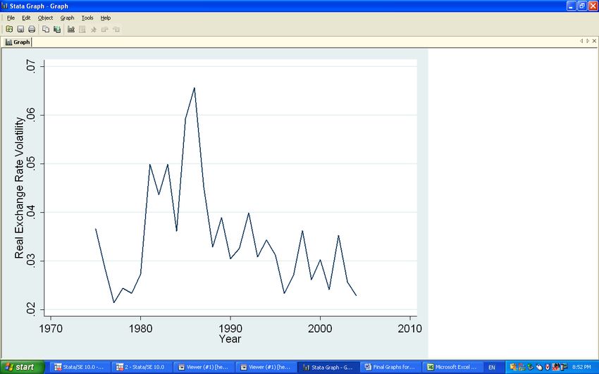
Does Capital Control Policy Affect Real Exchange Rate Volatility?
                             A Novel Appr oac h Usin g Pr op ens ity Sc ore M atching

T A B L E     O F     C O N T E N T S

Acknowledgements                                                                        3

Abstract & Keywords                                                                     4

       1     Introduction                                                               5

       2     Literature Review                                                          8

                2.1     The Relationship Between Capital Controls and Real
                        Exchange Rates                                                  8

                2.2     Capital Control Indices                                         11

                2.3     Propensity Score Matching Using Leuven and
                        Sianesi’s (2003) PSMATCH2                                       15

       3     Data Description                                                           18

                3.1     Real Exchange Rate Volatility                                   18

                3.2     Financial Openness                                              20

                3.3     Matching Variables Used for the Propensity Score                20

       4     Empirical Specification                                                    23

                4.1     Capital Control Policy Changes and Real Exchange
                        Rate Volatility                                                 24

                4.2     Treatment Effects of Capital Control Policy Changes             26

       5     Concluding Remarks                                                         29

Tables & Figures                                                                        30

References                                                                              38

                                                                                             2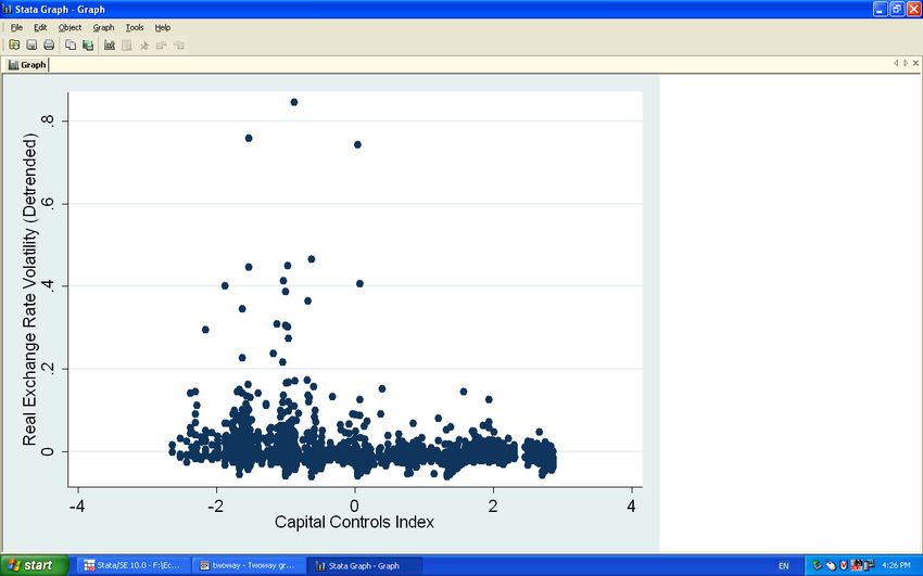
Does Capital Control Policy Affect Real Exchange Rate Volatility?
                            A Novel Appr oac h Usin g Pr op ens ity Sc ore M atching

A C K N O W L E D G E M E N T S

       I would like to thank my faculty advisor Dr. Craig Burnside for his patience, support,

and guidance throughout the academic year in preparation of this Honors Thesis. I would

also like to thank Dr. Michelle Connolly, Dr. Edward Tower, as well as my peers in the Fall

2007 Honors Research Seminar whose invaluable contributions helped form this project in

its initial stages. As well, thanks to Joel Herndon and Senghwa Rho at the Duke University

Library Data Services Department without whom it would have been impossible to work

with the novel statistical techniques discussed in this paper. Finally, thanks to Paul

Dudenhefer at the Department of Economics at Duke University, Mark Thomas at the

Duke University Library, Leonardo Bartolini at the Federal Reserve Bank of New York, and

Shenyang Guo at the School of Social Work of the University of North Carolina at Chapel

Hill, without whom this project would not have been the success I wished it to be.

                                                                                           3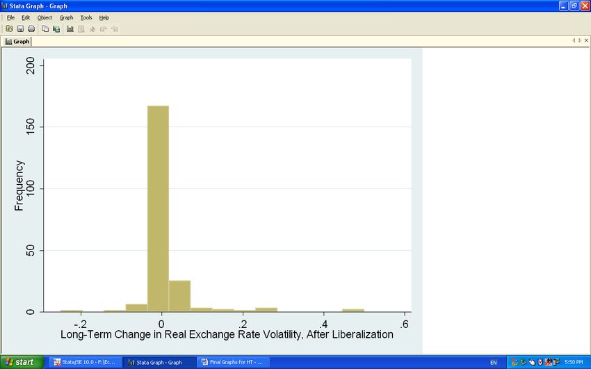
Does Capital Control Policy Affect Real Exchange Rate Volatility?
                             A Novel Appr oac h Usin g Pr op ens ity Sc ore M atching

A B S T R A C T

        Propensity score matching is a statistical technique recently introduced in the field of

economics, which researchers use to assess the treatment effect of policy initiatives. In this

study I use propensity score matching to analyze the treatment effect of capital control

policy on real exchange rate volatility. I find the treatment effect of adopting relatively liberal

capital controls is a decrease in real exchange rate volatility. This is the first empirical study

to provide insight into the causal relationship between capital controls and real exchange

rates, which may be crucial to macroeconomic policy decisions for emerging economies such

as China.

K E Y W O R D S

        Capital controls, real exchange rate, treatment effects, propensity score matching.

                                                                                                 4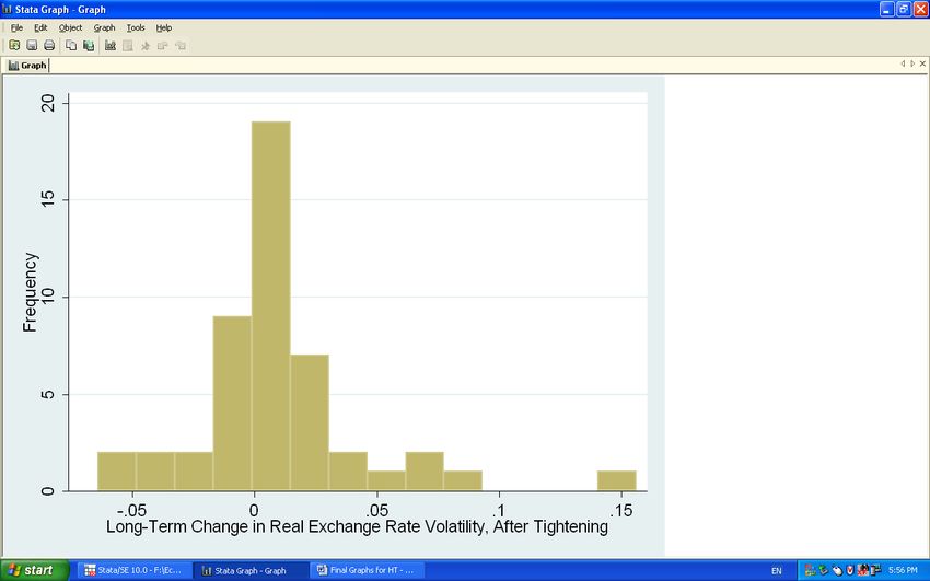
Many in China fear that the removal of capital controls that restrict the
                    ability of domestic investors to invest abroad or to sell and purchase
                    foreign currency could cause a destabilization of the whole system.

                                                                         - Alan Greenspan
                                                                         The Wall Street Journal, March 2, 2004

1.        I N T R O D U C T I O N

          Until recently it would have been impractical to empirically explore the validity of

China’s fears that the liberalization of capital controls would cause a “destabilization of the

whole system,” and in particular an increase in the volatility of the real exchange rate.1

Because the degree of capital controls is endogenously determined, traditional econometric

methods such as linear regression are unreliable in assessing the causal relationship between

capital control liberalization and real exchange rate volatility. Moreover, an experiment in

which countries are randomly assigned to liberalize or maintain their level of capital controls

is simply infeasible.

          In this paper I apply Leuven and Sianesi’s (2003) method of propensity score

matching to determine the treatment effect of capital control policy on real exchange rate

volatility. The traditional approach to dealing with the endogenaiety problem in empirical

macroeconomics is to use an instrumental variables method. However, one problem with

such methods is the difficulty of finding instruments that are both valid and relevant. As an

alternative to these methods, Leuven and Sianesi (2003) developed propensity score

matching, a novel econometric procedure that takes a different approach to solving the

endogenaiety problem. Essentially, their Stata module PSMATCH2 creates ‘couples’ from

1
  Real exchange rate volatility is one of many macroeconomic indicators of stability that could have been measured in this
study. It is nonetheless of particular concern for influential export-based emerging countries such as China given that past
declines in exports have been formally attributed to periods of increased real exchange rate volatility (Rose 2000; Iwatsubo
and Karikomi 2006). In practical terms, high real exchange rate volatility had directly affected the South Korean steel and
chemical industries in the 1990s.

                                                                                                                           5
data points by matching ‘male’ data points (countries that adopted a particular policy) with

‘female’ data points (countries that did not adopt the policy), based on their similar propensity

to make a change in policy. In my case, I study the decision to liberalize capital controls. The

treatment effect of capital control liberalization is, therefore, the average of the differences in

real exchange rate volatilities between the ‘male’ and ‘female’ data points of each ‘couple’.

        I find that the treatment effect of capital control liberalization is a decrease in real

exchange rate volatility. This result is reinforced in my second finding that capital control

tightening causes an increase in real exchange rate volatility. Although it is impossible to achieve

statistical significance at the 95% level in most propensity score matching tests with

PSMATCH2, I can be confident of these results at the 90% level. Moreover, correlations

and additional statistical tests examining long-run real exchange rate volatility following

changes in capital control policy are consistent with the results discovered using the

propensity score matching technique.

        The causal relationship discovered in this study is especially pertinent to emerging

economies such as China. Despite the desire to self-insure against macroeconomic instability

and massive capital outflows characteristic of the 1997 Asian financial crisis (Bartolini and

Drazen 1997), emerging economies with tight capital control policies are expected to

eventually follow the global trend of increasingly liberalized capital controls that began in the

1980s. On the basis that capital controls inhibit the most efficient use of economic

resources, Edwards (1999) notes that “at the practical policy level the debate has centered

not so much on whether capital controls should be eliminated, but on when and how fast this

should be done.” Therefore if the results of this study are indeed valid where the treatment

effect of capital control liberalization is an increase in macroeconomic stability (and not less

                                                                                                  6
stability as per China’s hypothesis) then the policy implication of this study is large enough
to warrant more careful empirical and theoretical consideration in the field.
Beyond the important policy implications, my research is novel in its use of the
propensity score matching technique and Chinn and Ito’s (2007) intensity-modified ordinal
index of de jure capital controls, KAOPEN. Although there has been ample research in the
past decade with regard to the advantages and effects of capital controls, the literature is
largely empirical2 and limited to a collection of case studies on characteristic countries3
concerned most often with the impact of such controls on growth, inflation and capital
flows. Edwards (1999) explains that economists have been reluctant to incorporate indices
of capital controls into their research because of the difficulty in documenting subtle
differences between de jure capital controls across multiple countries and a significant period
of time. Nevertheless, Chinn and Ito’s (2007) ordinal index of capital controls is the first to
enable accurate and simultaneous empirical measurements of relatively subtle changes in
capital control policy across 161 countries in a time period of 35 years. As one of the first
studies to incorporate Chinn and Ito’s (2007) novel measure of financial openness, this
research is unique not only in the methodology it uses to discuss treatment effects, but also
in its comparative study of capital control policy across multiple countries and a broad
period of time.
The remainder of this paper is organized as follows: Section 2 presents the relevant
literature on capital control indices preceding the creation of Chinn and Ito’s (2007)
KAOPEN measure of financial openness, as well as an explanation of the intuition behind
Leuven and Sianesi’s (2003) propensity score matching tool for Stata, PSMATCH2. Section
2
As documented in Frenkel (2001) and Edwards (1999).
3
For example: Chile, Mexico, Uruguay, Colombia by Edwards (1999) and New Zealand, Portugal, Ireland, Israel by Alfaro
and Kanczuk (2004).
73 describes the data to be used herein. Section 4 explores the methodology, results, and
some interpretation. Section 5 concludes.
2. L I T E R A T U R E R E V I E W
Although this is the first study to directly explore the treatment effect of capital
control policy on real exchange rate volatility, there are three elements in particular which
require further elaboration in the literature review. First I describe the function of capital
controls, and discuss previous research that establishes a relationship between capital
controls and real exchange rates. Second, I provide a brief history of capital control indices
leading up to Chinn and Ito’s (2007) novel measure of financial openness. In so doing, I
establish why Chinn and Ito’s (2007) KAOPEN variable is the first to enable accurate and
simultaneous empirical measurements of relatively subtle changes in de jure capital control
policy across multiple countries. Third, I explain the intuition behind Leuven and Sianesi’s
(2003) propensity score matching tool PSMATCH2, which I use to study the treatment
effect of capital control policy changes on real exchange rate volatility. Additionally, I
describe two recent studies that also use PSMATCH2 as their central empirical method.
2.1 The Relationship Between Capital Controls and Real Exchange Rates
Capital controls are financial market policies designed to limit or redirect
international transactions of investment-related financial instruments. These controls have
generally been used for a variety of reasons: to support government attempts to broaden the
tax base for a capital levy, sustain fixed or managed exchange rate policy, prevent capital
outflows by making them cost-prohibitive, or promote macroeconomic stability. Bartolini
and Drazen (1997) note that some form of capital control policy was used in 3 of 24 OECD
8countries4 and in as many as 126 of 158 developing countries in 1995. Two particular
examples of capital control policy are the Chilean Encaje and the U.S. Interest Equalization Tax.
Between 1991 and 1998, the Chilean Encaje was put in place to restrict capital inflows
for three reasons. First, the Encaje attempted to promote macroeconomic stability by limiting
potentially volatile inflows that could be drained in a crisis. Second, it attempted to reduce
destabilization by avoiding capital that could distort incentives in financial markets. Third, it
attempted to reduce monetary expansion, which in turn decelerates domestic inflation, and
inhibits rapid appreciation of the real exchange rate.
The rationale for capital controls in the U.S. was very different than in Chile. The
U.S. Interest Equalization Tax between 1963 and 1974 targeted capital outflows to correct a
balance of payments deficit. The objective of the U.S. Interest Equalization Tax was to reduce
the demand for foreign assets, without having to either use contractionary monetary policy
or devalue the local currency, thus allowing for inflation to be higher.
The Chilean Encaje and the U.S. Interest Equalization Tax suggest that capital controls
can vary considerably in both their objective and implementation. Because capital controls
can take many forms – from taxes to restrictions and outright prohibitions on the cross-
border trade of assets – it can be difficult to model the effects of these policies.
Nevertheless, economists broadly agree that while capital controls may be useful under
certain circumstances they are still fundamentally taxes on the movement of capital, which
are analogous to tariffs on goods in that they both detract from economic efficiency.
Specifically, capital controls can be detrimental when they prevent financial resources from
being used where they are needed most (Neely 1999). Basic theory and empirical studies
follow this intuition.
4
Greece, Norway and Turkey.
9Barro (1997) explains as per the neoclassical model, that in a closed economy the
capital stock is expected to grow according to a concave function, very slowly approaching a
long-run steady state. As illustrated in Figure 1, if the capital account were opened the capital
stock would rapidly approach the steady state, net of adjustment costs.5 Rapid adjustment of
the capital stock to the long-run steady state promotes a more efficient allocation of global
capital because of the higher rate of return in the previously closed economy. These capital
inflows are beneficial because they presumably increase growth, employment opportunities,
and living standards in the liberalizing country. However, the potential consequences of this
adjustment may also deter certain countries from liberalizing their capital controls.
Fundamentals suggest that a rapid increase in capital inflows to the steady state
would also generate an increase in aggregate expenditure, which would in turn give rise to
increased pressure on domestic prices, cause an appreciation of the real exchange rate, and
thus imply a loss of international competitiveness. Edwards’ (1999) Latin American case
studies provide empirical evidence that an increase in capital flows is associated with an
appreciation of the real exchange rate. Moreover, Edwards (1999) uses a Granger causality
test to show that it is not possible to reject the null hypothesis that increased capital flows
cause real exchange rate movements.
Although these theories suggest that there are immediate benefits (e.g. an increase in
available capital) and costs (e.g. macroeconomic overheating) to capital control liberalization,
they nonetheless provide no explanation of how changes in policy affect macroeconomic
stability, or more specifically real exchange rate volatility. Edwards (1999) and Alfaro and
Kanczuk (2004) have commented in Latin American case studies that a short period of real
5
Bartolini and Drazen (1997) extend the basic model where liberal policy allowing capital outflows sends a favorable signal
to investors that intrinsically triggers additional capital inflows, thereby increasing the long-run steady state. Bartolini and
Drazen’s (1997) model is consistent with the experiences of several Latin American and European countries that have
liberalized their capital controls.
10exchange rate volatility tends to follow the liberalization of capital controls in most
countries, presumably until capital flows stabilize at a steady state.6 Nevertheless, both
studies suggest that beyond the initial period of capital adjustment, differences in real
exchange rate volatility before and after the liberalization are largely unclear. Edwards (1999)
also notes that even if there had been a greater increase in post-policy real exchange rate
volatility, it would still be difficult to attribute the increase in volatility to the change in policy
because volatility is on average much higher in Latin America than in the rest of the world.
Therefore, in order to gain a better understanding of how capital controls affect
macroeconomic stability, it may be necessary to look beyond case studies, and use an index
of capital controls to simultaneously study subtle policy changes across a broad range of
countries and time.
2.2 Capital Control Indices
Edwards (1999) and Rogoff (1999) argue that our understanding of the effects of
capital control policy is limited by our ability to construct an accurate index of capital
controls. In effect, our basic notion of capital controls is largely the product of careful case
studies on characteristic countries such as Chile, Colombia, Germany, Malaysia, Mexico, and
Portugal.7 Although capital control indices could allow the simultaneous study of capital
control policy across a broad range of countries and time, researchers have been reluctant to
use indices for a few reasons. Specifically, past indices have failed to account for the intensity
of capital controls, the subtlety regarding the direction of the controls, and most importantly
6
Edwards (1999) proposes that relaxing the external credit constraint may have two implications: a long-run increase in the
sustainable volume of capital flows and a short-run overshooting of capital into the economy. Although the long-run effect
is dependent on the stock demand for the country’s securities by foreigners, the real rate of growth, and the world interest
rate, a short-run overshooting may occur because capital inflows can exceed long-run equilibrium volume while the new
capital is dispersed into the economy. Although the theory is admittedly circumstantial, the author suggests this short-run
overshooting of capital may have caused the increase in real exchange rate volatility following capital control liberalization.
7
Edwards (1999), Neely (1999), and Alfaro and Kanczuk (2004),
11the efficacy with respect to discerning between de facto and de jure controls. In this
subsection, I discuss the evolution of capital control indices. I also explain the construction
of Chinn and Ito’s (2007) KAOPEN measure of financial openness, which I use in this
study.
2.2.1 Binary Indices Preceding Chinn and Ito (2007)
The primary source from which capital control indices are constructed is the
International Monetary Fund’s Annual Report of Exchange Arrangements and Exchange Restrictions
(AREAER). Published annually since 1967, the AERAER also offers a summary table with
binary indicators for four types of de facto controls: (a) multiple exchange rates, (b)
restrictions on current account transactions, (c) restrictions on capital account transactions,
and (d) regulatory requirements on the surrender of export proceeds. Eichengreen (1998)
was among the first to use a capital control index in his research, combining the binary
indicators in the AREAER summary tables to create a four-point scale of capital controls.
Eichengreen (1998) used the index to suggest that contrary to the general consensus
in the field, there was no trend of capital control liberalization over time. This result was
received with much skepticism. Edwards (1999) among others used Eichengreen’s (1998)
study to illustrate the danger of generalizing complex capital controls in a simple four-point
scale. He argued that the results of Eichengreen’s (1998) study were misleading because the
index failed to capture differences in the intensity of capital controls. He also reasoned that
the index did not account for whether the de facto policies recorded in the AREAER
effectively restricted capital flows, or if the controls were regularly circumvented. For
example, Edwards (1999) explains that according to the four AREAER binary indicators,
Chile, Mexico and Brazil were subject to the same degree of capital controls between 1992
and 1994. In reality, not only did capital control policy undergo important changes within
12these countries, but also the controls between these countries were extremely different.
Brazil employed an arcane list of restrictions on inflows and outflows, while Chile directed
its Encaje principally at short-term inflows, and Mexico in practice had free capital mobility.
In 1998 the AREAER expanded the four subcategories in its summary table and
now offers fourteen binary indicators for de facto controls on: capital market securities,
collective investment instruments, commercial credits, foreign direct investment, and real
estate transactions among others. Johnston and Tamirisa (1998) extrapolate these fourteen
disaggregated binary indicators back in time through 1996 to create a new capital control
index. Miniane (2004) uses the same approach as Johnston and Tamirisa (1998), expanding
the index to include data through 1983, but for only 34 countries. Although more accurate
than the four-point scale of capital controls, Johnston and Tamirisa (1998) and Miniane’s
(2004) indices are still unadjusted for intensity and efficacy. Moreover, they are either
severely limited by the number of years (Johnston and Tamirisa 1998) or number of
countries (Miniane 2004) they exclude. In summary, these indices are both imperfect as they
still do not allow the accurate and simultaneous study of capital control policy worldwide.
Chinn and Ito (2007) create the first intensity-modified measure of financial
openness. They also expand the range of data, providing capital control measures for 181
countries from 1970 through 2005. Moreover, unlike the original four-point measures of
capital controls, the KAOPEN variable correctly demonstrates the gradual liberalization of
capital controls across all countries in each decade since 1970.8 Because of these
improvements, the KAOPEN variable should provide a relatively accurate representation of
capital controls in this study. In the next section, I discuss the construction of KAOPEN.
8
KAOPEN demonstrates the gradual liberalization of capital controls in each decade (1970-79, 1980-89, 1990-99, 2000-05)
for the aggregate of countries as well as for subgroups of (a) Central/Eastern European (ex-planning) countries, (b) South
Asian/Middle Eastern/African countries, (c) emerging countries, (d) less-developed countries, and (e) industrial countries.
Asia-Pacific countries demonstrate liberalization in each period except from 2000-05. However, this apparent tightening of
capital controls is consistent with policy initiatives that followed the Asian Financial Crisis beginning in 1997. See Figure 3.
132.2.2 Construction of Chinn and Ito’s (2007) KAOPEN Variable
The following section on the construction of the KAOPEN variable closely follows Chinn and Ito’s
(2007) original discussion.
Chinn and Ito (2007) derive their measure of financial openness by assessing the
intensity of each of the four categories of controls listed in the original AREAER summary
tables: (k1) multiple exchange rates, (k2) restrictions on current account transactions, (k3)
restrictions on capital account transactions, and (k4) regulatory requirements on the
surrender of export proceeds. Because the index focuses on financial openness rather than the
degree of restriction, the highest-intensity controls are assigned the minimum value, while non-
existent controls are assigned the maximum value. Furthermore, in order to reflect the delay
(latency period) for a new policy to realize its full effect, Chinn and Ito (2007) use a five-year
moving average for restrictions on capital account transactions (k3). In other words, instead
of using k3 at time t to construct KAOPENt, they instead use SHAREk3.
(1) SHAREk3 = (k3,t + k3,t-1 + k3,t-2 + k3,t-3 + k3,t-4 ) / 5.
The authors use principal components analysis to reduce the multidimensional data
set [k1,t, k2,t, SHAREk3,t, and k4,t] to a single dimension KAOPENt. In principal components
analysis each attribute of the data set is first mean centered. Then an orthogonal linear
transformation converts the data set to a new coordinate system so that the greatest variance
in any attribute comes to lie on the first coordinate, or the first principal component. By
definition, the aggregate measure of financial openness KAOPENt including all years and
countries has a mean of zero. Its value also increases when capital controls are more liberal.
Chinn and Ito (2007) use the first eigenvector for KAOPEN to demonstrate that
their measure of financial openness is not merely driven by changes in the moving average of
restrictions on capital account transactions (SHAREk3). As per the mathematical definition
14of an eigenvector, each component of the eigenvector represents the weight of that
particular attribute in determining KAOPEN. Because the first eigenvector for KAOPEN is
(k1,t, k2,t, SHAREk3,t, k4,t) = (0.25, 0.52, 0.57, 0.58), it is reasonable to deduce that the
inclusion of k1,t, k2,t, and k4,t in the index allows it to more accurately represent the intensity
of the capital controls. Chinn and Ito (2007) argue that the existence of different types of
restrictions (k1, k2, or k4) alongside k3 signals more intense capital controls. For example, a
county might support its capital account controls (k3) by imposing restrictions on current
account transactions (k2) to prevent the private sector from bypassing the capital controls.
In summary, Chinn and Ito’s (2007) measure of financial openness is arguably an
improvement over previous binary indices because of its vast coverage of countries and
time. More importantly it considers the intensity and not simply the existence of capital
controls. Therefore, I am reasonably confident that KAOPEN is the measure of capital
controls that most accurately reports their existence and intensity worldwide and across time.
2.3 Propensity Score Matching Using Leuven and Sianesi’s (2003) PSMATCH2
The ultimate goal of this study is to evaluate the treatment effect of changes in
capital control policy on real exchange rate volatility. If changes in capital control policy were
exogenous, it would be possible to estimate the average treatment effect on the treated
(ATT) simply by subtracting the average volatility of non-treated countries from the average
volatility of treated countries.
(2) ATT = E[Pi1Ci=1] - E[Pi0Ci=1]
C = dummy for country of observation
Pi1Ci=1 = volatility given a change of policy in country 1
Pi0Ci=1 = volatility in country 1 if there had not been a change in policy
The above construction is analogous to a clinical experiment where the left-hand term
(Pi1Ci=1) represents the group of subjects randomly assigned to take the test drug (change in
15capital controls), and the right-hand term (Pi0Ci=1) represents the group of subjects randomly
assigned to the placebo (no change in capital controls). However, because changes in capital
control policy are nonrandom it is impossible to determine what the volatility would have
been in a given country, had that country not changed its capital control policy. Moreover, it
is implausible in the macroeconomy to design an experiment to test this treatment effect by
randomly assigning countries to either change or maintain their capital control policy.
Given that capital control policy is endogenous to other macroeconomic factors, we
would generate biased estimates by simply subtracting the average volatility of countries that
changed their capital controls from the average volatility of countries that maintained their
policy. In other words, because capital control policy is systematically correlated with a set of
macroeconomic factors that also affect volatility, we are confronted with the problem of
selection on observables. In this study I use Leuven and Sianesi’s (2003) propensity score
matching tool for Stata (PSMATCH2) to address the issue of self-selection in policy
adoption.
The intuition for propensity score matching is to recreate Equation 2 with a mock
control group to simulate a randomized experiment. If we assume that conditional on
attributes Xi the outcomes are independent of the particular country Ci, then it is also possible
to observe the average treatment effect with the following equation:
(3) ATT = E[Pi1Ci=1, Xi] - E[Pi0Ci=0, Xi]
Pi1Ci=1, Xi = volatility in country 1 which changed its policy, under
conditions Xi
Pi0Ci=0, Xi = volatility in country 0 which maintained its policy,
under the same conditions Xi
Using the mock experiment in Equation 3, it is possible to estimate the average treatment
effect by creating ‘couples’ from data points by matching ‘male’ data points (countries that
liberalized capital controls) with ‘female’ data points (countries that maintained capital
16controls) conditional on having the same attribute values (Xi) to eliminate the selection bias.
The average treatment effect is the average difference in volatility between the ‘male’ and
‘female’ data points of each ‘couple’.
In order to facilitate the matching process as the number of matching variables in Xi
increases, Leuven and Sianesi (2003) transform the values for the matching variables
(attributes) in Xi into a propensity score.9 A propensity score is simply the probability of a
change in capital control policy given country Ci’s set of attribute values Xi. In PSMATCH2,
the propensity to make a change in capital control policy is estimated using a logit model.
Matching the ‘couples’ using propensity scores instead of with raw attributes changes
Equation 3 to the following:
(4) ATT = E[Pi1Ci=1, pr(Xi)] - E[Pi0Ci=0, pr(Xi)]
Pi1Ci=1, Xi = volatility in country 1 which changed its policy, given
the propensity to change its policy pr(Xi)
Pi0Ci=0, Xi = volatility in country 0 which maintained its policy,
given the same propensity to change its policy pr(Xi)
Following the above discussion on the intuition for propensity score matching, there
are three basic steps in Leuven and Sianesi’s (2003) PSMATCH2 tool. First, PSMATCH2
uses a logistic regression to predict the propensity to make a change in capital controls.
Second, PSMATCH2 matches data ‘couples’ based on their propensity scores and a given
caliper, which is the maximum allowable difference in propensity between the ‘male’ and
‘female’ components of each ‘couple’. Third, PSMATCH2 determines the treatment effect
by averaging the difference in volatility between the ‘male’ (treated) and ‘female’ (untreated)
data points of each ‘couple’.
9
Rosenbaum and Rubin (1983) first proposed that treated units and control units could be matched with propensity scores
instead of using a set of basic attributes Xi. However, Leuven and Sianesi (2003) constructed the first working model for
propensity score matching in Stata.
17Recent papers that use Leuven and Sianesei’s (2003) propensity score matching tool
include Lin and Ye (2007 forthcoming) and Guo et al. (2005). Lin and Ye (2007) use
PSMATCH2 to show that inflation targeting does not significantly affect either inflation or
inflation variability. Guo et al. (2005a) use PSMATCH2 to evaluate the effectiveness of
substance abuse services for child welfare clients. Guo (2005b) also provides a guide to the
Stata code for PSMATCH2.
3. D A T A D E S C R I P T I O N
In this section I describe the three principal elements of data used in this study. First
I define real exchange rates, and explain the calculation of real exchange rate volatility.
Second, I present summary statistics for the central explanatory variable: Chinn and Ito’s
(2007) measure of financial openness. Note that the construction of KAOPEN is discussed
in detail in Section 2.2.2. Third, I describe the matching variables used in the logistic
regression to determine the propensity to change capital control policy.
3.1 Real Exchange Rate Volatility
The central dependent variable in this study is real exchange rate volatility. I begin
with normalized and trade-weighted monthly real effective exchange rates (RERi,t) based on
relative consumer prices from the International Monetary Fund Statistical Database. The
IMF defines RERi,t as follows.
(5)10 δij,t = Δln(eij,t)
(6)11 πi,t = Δln(Pi,t)
(7)12 εij,t = δij,t + πj,t – πi,t
(8)13 φi,t = Σ Jij · εij,t
10
e is exchange rate between country i and its trading partners j.
11
πi,t is inflation in country i at time t. P is the price level.
12
εij,t represents Δln(RER) between countries i, j at time t.
13
J is the trade weight for country i of country j. Note that Jij ≠ Jji.
18(9) φi,t = ln(RERi,t) – ln(RERi,t-1)
(10) RERi,t = RERi,t-1 · exp(φi,t)
Although IMF data is available through 1970, it is extremely limited in the number of
countries through 1975. Therefore, I only consider data in the period from 1975-2005. For
this period data is offered for 91 countries. Note that although the IMF collects data for
more than 180 countries, many choose not to disclose the necessary information to
determine historical monthly real effective exchange rates.
I convert monthly values of RERi,t into annual measures of real exchange rate
volatility (RERvoli,t) by taking the standard deviation of the natural logarithm of the monthly
RERi,t values within each year. In other words, my measure of real exchange rate volatility is
the percentage deviation from the average real exchange rate in any given year. The
mathematical formula for RERvoli,t is as follows.
(11) µi,t = (1/12) Σ ln(RERi,t)
(12) σi,t = √ [ (1/12-1) Σ (ln(RERi,t) – µ)2 ]
σi,t = RERvoli,t
Finally, I also create a de-trended measure of real exchange rate volatility (RERvôli,t) by
removing the time and country-specific fixed effects according to the following formula.
(13) RERvôli,t = RERvoli,t – Coûntryi – Yêart
By defining real exchange rate volatility (RERvoli,t) as the percentage deviation from
the average in each sub-period, I am implicitly removing the long-term trend from my
calculation of volatility. Although Clark et al. (2004) note that there is no consensus in the
field on how to define volatility; the convention is nonetheless to measure deviations from
long-term trends. Rose (2000) justifies that the negative macroeconomic effects associated
with volatility are characteristic of deviations from long-term trends rather than changes
19which are consistent with the trend. Therefore, I am confident that my definition of real
exchange rate volatility accurately captures macroeconomic instability.
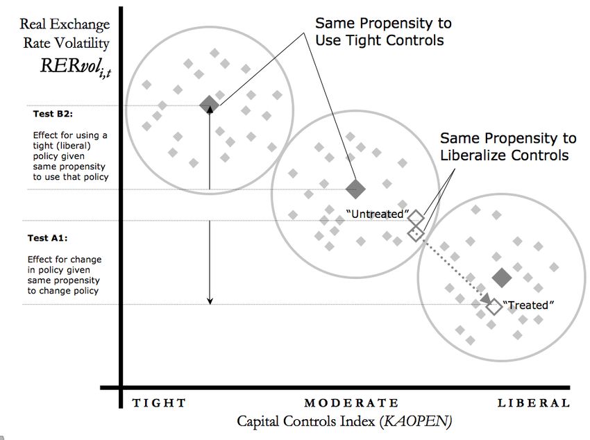
Summary statistics for real exchange rate volatility (RERvoli,t) are presented in Table
1. Additionally, real exchange rate volatility versus time is plotted in Figure 2.
3.2 Financial Openness
The central explanatory variable is Chinn and Ito’s (2007) KAOPEN measure of
financial openness. By construction, KAOPEN is positive when capital controls are relatively
liberal, and negative when capital controls are tight. Table 1 includes summary statistics for
the subset of 91 countries from 1975-2005 used in this study (limited by IMF data on real
exchange rates) alongside the summary statistics for the complete 35-year index of all 181
countries. Although I use less than half of Chinn and Ito’s (2007) original data (2422 of 5102
values) I am confident from the summary statistics that I have a representative sample.
I graph average financial openness versus time in Figure 3 to emphasize the accuracy
of the KAOPEN variable in reflecting de jure capital controls. Recall from Section 2.2.1 that
Chinn and Ito’s (2007) index is unique in that it correctly demonstrates the global
liberalization of capital controls since the 1970s.
3.3 Matching Variables Used to Determine the Propensity Score
I use nine additional matching variables (covariates) in a logistic regression to
determine the propensity for country i at time t to make a change in capital controls. These
variables are: (a) the natural logarithm of real GDP per capita, (b) the natural logarithm of
population, (c) openness to cross-border trade, (d) capital inflows, (e) months of foreign
reserves, (f) debt as a fraction of GDP, (g) CPI inflation, (h) a binary variable for floating
exchange rate mechanism, and (i) a binary variable for whether a currency crisis is taking
20place. I discuss the construction, sources and rationale for including each of these variables
below. I also provide summary statistics for these variables in Table 1.
3.3.1 Natural Logarithm of Real GDP Per Capita (lnGDPni,t)
The source for real GDP per capita data is the Penn World Table. I calculate the
natural logarithm of real GDP per capita from the raw data before including it in the logistic
regression to calculate the propensity for changes in capital control policy. I include this
measure in the propensity calculation because of the tendency for developed countries to
have more liberal capital controls. For example, Bartolini and Drazen (1997) note that only 3
of 24 OECD countries had in place some form of capital control policy in 1995, while 126
of 158 developing countries used capital controls that same year.
3.3.2 Natural Logarithm of Population (lnPOPi,t)
I calculate the natural logarithm of population from raw population data available in
the Penn World Table. I include population because extremely small countries may be more
reliant on foreign capital, and would therefore be more likely adopt liberal policies with
respect to capital flows.
3.3.3 Openness to Cross-Border Trade (OPENTRDi,t)
(14) OPENTRDi,t = (Imports + Exports) / GDP
Openness to cross-border trade is defined above as the sum of imports plus exports,
divided by GDP. Data for trade openness is available from the World Bank World Tables.
Hau (2002) presents a model in which smaller real exchange rate movements follow supply-
side shocks if the economy is more open to international trade. Also, Quinn (1997) notes
that openness to cross-border trade is moderately correlated with capital account openness.
Therefore, it is worthwhile to consider trade openness in the propensity calculation.
213.3.4 Capital Inflows (CAPFi,t)
I use data from Rose (2000) to determine capital inflows. The measure includes
foreign direct investment, portfolio investments, and loans. I include a variable for capital
flows in the propensity calculation because the volume and volatility of capital flows are
important factors in the determination of capital control policy (Neely 1999)
3.3.5 Months of Foreign Reserves (RESmoi,t)
Months of foreign reserves are defined as the total value of foreign reserves divided
by the value of imports per month. This data is available in Rose (2000). I include this
variable because low reserves may signal a currency crisis and may also lead to a tightening of
capital control policy as a defensive mechanism.
3.3.6 Debt as a Fraction of GDP (DEBTi,t)
The measure of debt divided by GDP is also available in Rose (2000). I include this
data in the propensity calculation for the same reason as GDP per capita. That is, more
developed countries with less debt may be more likely to have liberal capital control policies.
3.3.7 CPI Inflation (CPIinfi,t)
Data for CPI inflation is available from the World Bank World Tables. I include this
data because inflation is an important signal of macroeconomic stability. Moreover, Edwards
(1993) notes that market-distorting policies such as capital controls are often related to high
levels of inflation.
3.3.8 Binary Variable for Floating Exchange Rate Mechanism (EXRbini,t)
I use a binary variable for de jure floating exchange rate mechanisms available in
Rose (2000). The variable takes on a value of 1 if the exchange rate is floating, and 0 if the
22exchange rate is fixed, managed, or intermediate. This measure is based on data from the
IMF Annual Report of Exchange Arrangements and Exchange Restrictions. I include the
exchange rate mechanism because the exact way in which capital inflows cause a real
exchange rate appreciation is dependent on the nature of the exchange rate system. With a
fixed exchange rate, the increased availability of foreign resources will result in an
accumulation of reserves, monetary expansion, and increased inflation. These factors will in
turn, eventually cause the real exchange rate to appreciate. Conversely, under a floating
exchange rate system, nominal and real exchange rate appreciations occur simultaneously
(Frenkel et al. 2001). Moreover, Quinn (1997) notes that the use of fixed exchange rates is
often coupled with the use of capital controls.
3.3.9 Binary Variable for Currency Crises (CCRbini,t)
I use Rose’s (2000) binary variable for currency crises which takes on a value of 1 if a
currency crisis is occurring and 0 if not. The variable is constructed from journalistic and
academic episodes of past currency crises. I include this variable because currency crises are
an important determining factor of capital control policy, as evidenced after the Asian
Financial Crisis when Malaysia, Thailand, and Indonesia among others tightened their
controls (as per Palma 2000 and also reflected in Chinn and Ito’s KAOPEN index).
4. E M P I R I C A L S P E C I F I C A T I O N
In this section I discuss two sets of tests to explore the relationship between real
exchange rate volatility and capital control policy. In Section 4.1, I present the results of
preliminary tests, including the correlation of financial openness and real exchange rate
volatility. I also calculate a measure of long-term volatility following different types of
changes in capital control policy. In Section 4.2, I explore whether the changes in capital
23controls caused the changes in volatility that I observed in the preliminary tests. In order to
discuss the treatment effect of capital control policy on real exchange rate volatility, I apply
Leuven & Sianesi’s (2003) propensity score matching technique to the data. Specifically, I
use propensity score matching to answer two questions: (a) what is the treatment effect of
changing (liberalizing or tightening) capital control policy on real exchange rate volatility; and
(b) what is the treatment effect of using tight or liberal capital controls on real exchange rate
volatility?
4.1 Capital Control Policy Changes and Real Exchange Rate Volatility
In order to understand the basic relationship between capital controls and real
exchange rate volatility, I begin by exploring the correlation between relative financial
openness (KAOPENi,t) and de-trended14 real exchange rate volatility (RERvôli,t) in Figure 4.
It is important to emphasize that financial openness is a relative measure because Chinn and
Ito’s KAOPEN index is ordinal rather than cardinal. The correlation coefficient is -0.181,
suggesting a weak (yet still statistically significant15) negative relationship between the relative
degree of capital controls and real exchange rate volatility. Note that the statistically
significant negative relationship is still preserved (ρ=-0.176) when outliers with de-trended
volatilities greater than 20% are removed from the calculation. The implication from this test
is that countries with more liberal capital controls are associated with less real exchange rate
volatility. Nevertheless, because financial openness and real exchange rate volatility are both
endogenous, it is impossible to infer causality from this correlation alone.
In a second preliminary test, I examine the long-term change in volatility for
countries that make considerable changes in their capital control policy. I define long-term
14
I remove the time and country-specific fixed effects from real exchange rate volatility (RERvoli,t) to calculate de-trended
real exchange rate volatility (RERvôli,t). Please refer to Section 3.1 for more details.
15
p < 0.05
24change in real exchange rate volatility (ΔRERvolLTi,t) as the difference between the average
volatility for the three years prior to the policy change and the average volatility for the three
years following the policy change. The mathematical formula is as follows.
(15) ΔRERvolLTi,t = [ (RERvoli,t-3 + RERvoli,t-2 + RERvoli,t-1) / 3]
– [ (RERvoli,t + RERvoli,t+1 + RERvoli,t+2) / 3]
According to the construction of the long-term change in volatility variable, positive values of
ΔRERvolLTi,t signify a long-term decrease in volatility following the policy change, while
negative values signify an increase in volatility. In Figure 5a, I display the long-term change in
volatility at year t for all countries that significantly liberalized their capital controls during year
t by at least +0.5 standard deviations of the KAOPEN index.16 In Figure 5b, I display the
change in volatility for all countries that tightened their capital controls by at least -0.5SD of
KAOPEN.
I find that there is a statistically significant17 decrease in long-term real exchange rate
volatility of approximately 1% for countries that liberalized their capital controls in Figure
5a. Countries that tightened their capital controls in Figure 5b also experienced an average
decrease in long-term volatility of approximately 0.1%, but this result is not statistically
significant at the 95% level. Although it makes sense that countries in Figure 5a experience a
decrease in long-term volatility after a market-promoting policy change, it is more difficult to
interpret the positive result for countries that made a market-interfering policy change in
Figure 5b. Nevertheless, even if long-term real exchange rate volatility were to improve on
average after a country tightens its capital controls, it is still impossible to determine from
this test whether the decision to tighten capital controls causes the decrease in volatility. In
16
The standard deviation of the KAOPEN index for the countries and years used in this study is 1.533. Therefore, in order
to examine changes greater than +0.5SD of KAOPEN, I consider data points where KAOPENi,t - KAOPENi,t-1 > 0.767.
17
p < 0.05.
25order to determine causality, I use Leuven and Sianesi’s (2003) propensity score matching
technique.
4.2 Treatment Effects of Capital Control Policy Changes
I use propensity score matching to reconsider the question of whether changes in
capital control policy cause changes in de-trended real exchange rate volatility. To simplify
the propensity score matching process, I consider capital control liberalization and
tightening separately.
In order to examine the treatment effect of capital control liberalization, I start a new
database, which only includes countries that maintained or significantly liberalized their
capital controls by more than 0.25SD of KAOPEN.18 According to the three basic steps in
Leuven and Sianesi’s (2003) PSMATCH2 tool, I first, use a logistic regression with the
matching variables listed in Section 3.319 to predict the propensity for countries to liberalize
their capital controls. Results for the logistic regression step are listed in Table 2. Next, I
repeat the data-matching step several times, varying the caliper (maximum allowable
difference in propensity scores between treated and untreated data points in each couple)
from 0.01 to 0.005, or approximately 0.1 standard deviations of the propensity score. Smaller
calipers ensure smaller differences in the propensity to liberalize between treated and
untreated data points for each couple. In the third step, PSMATCH2 determines the
treatment effect by averaging the differences in volatility between the treated and untreated
data points of each couple created in the second step. I repeat this process to determine the
18
In order to include only countries that maintained or liberalized their capital controls, I temporarily discard data points
where KAOPENi,t - KAOPENi,t-1 < 0. I define significant liberalizers or treated units as all data where KAOPENi,t -
KAOPENi,t-1 ≥ 0.25SD of KAOPEN (0.383). I define countries which maintained their capital controls or untreated units as
the remaining data where 0 ≤ KAOPENi,t - KAOPENi,t-1 < 0.25SD of KAOPEN (0.383).
19
The matching variables are: (a) the natural logarithm of real GDP per capita, (b) the natural logarithm of population, (c)
openness to cross-border trade, (d) net capital flows, (e) months of foreign reserves, (f) debt as a fraction of GDP, (g) CPI
inflation, (h) a binary variable for floating exchange rate mechanism, and (i) a binary variable for whether a currency crisis is
taking place. Details on the source and construction of these variables is available in Section 3.3
26treatment effect for tightening, using a new database that only includes countries that
tightened or maintained their capital controls. I list the results for these propensity score
matching tests in Table 3.
The average treatment effect for countries that tightened their capital controls is an
increase in real exchange rate volatility of approximately 2.5% in the year following the
policy change. Results are statistically significant at the 95% level for all calipers. The results
for liberalizers are more ambiguous. Although the average treatment effect for all calipers is
a decrease in real exchange rate volatility of approximately 0.1%, the effect is statistically
insignificant even at the 90% level. Therefore, while I can be certain that tightening capital
controls causes an increase in real exchange rate volatility, I cannot be certain that there is a
non-zero effect for the liberalization of capital controls.
In the second propensity score matching exercise, I explore the treatment effect of
simply having liberal, moderate, or tight capital controls. I define liberal capital controls as the
top third (with the greatest financial openness) of the KAOPEN index, moderate capital
controls as the middle third, and tight capital controls as the bottom third. This second
exercise is important because it explains whether the negative correlation between financial
openness and real exchange rate volatility (Figure 4) is caused by a country’s choice in capital
controls, or instead due to other macroeconomic factors.
I illustrate the difference between the first and second tests in Figure 6. The large
outlined diamonds depict the first experiment in which I determine the treatment effect for
capital control liberalization by calculating the difference in real exchange rate volatility
between countries that liberalized and countries that maintained their capital controls, given
the same propensity to liberalize their capital controls. The large solid diamonds depict the
second experiment in which I determine the treatment effect for using tight capital control
27policy by calculating the difference in volatility between countries that use tight and
countries that use moderate controls, given the same propensity to use tight controls.
In order to determine the treatment effect of simply having in place particular capital
control policies, I repeat the process described above for the first exercise. However, in this
variation of the test, I use separate data sets to explore the treatment effect for choosing
liberal instead of moderate capital controls, and for using tight instead of moderate controls.
I list the results for these tests in Table 2.
For all calipers, the treatment effect for using liberal instead of moderate capital
controls is an average decrease in real exchange rate volatility of approximately 1%. This
effect is significant at the 90% confidence level in all trials. Although the effect is more
ambiguous when a small caliper is used for countries that use tight capital controls, I can be
relatively confident from the trials with large and medium calipers that the use of tight
capital control policy causes countries to have higher real exchange rate volatility.
Specifically, the treatment effect for using tight instead of moderate capital controls is an
average increase in real exchange rate volatility of approximately 1%.
Considering the results of the two propensity score matching experiments together, I
am reasonably confident that using a relatively liberal capital control policy causes a country
to have lower real exchange volatility. Moreover, the treatment effect of further liberalization
is likely a decrease in real exchange rate volatility. I also find that choosing tight capital
controls as well as the act of tightening capital controls both cause increases in real exchange
rate volatility. The magnitude of the average treatment effect for these tests is a change in
real exchange rate volatility of approximately 1%. These results are consistent with the
neoclassical expectation that market-promoting policy is associated with better
macroeconomic stability.
285. C O N C L U D I N G R E M A R K S
In this study I use a novel statistical approach to determine the treatment effect of
capital control policy choices on real exchange rate volatility. I find that liberalizing capital
controls and maintaining a liberal policy are both associated with decreases in real exchange
rate volatility. Conversely, tightening capital controls and maintaining a tight policy are both
associated with increases in real exchange rate volatility. Although few tests are statistically
significant at the 95% level, the majority of tests show that that these results are significant at
the 90% level. In making a first attempt to understand the treatment effect of capital control
policy on real exchange rate volatility, this study will hopefully provide a directive for future
empirical and theoretical research to describe the mechanism by which the choice of capital
control policy affects the stability of the macroeconomy.
29Does Capital Control Policy Affect Real Exchange Rate Volatility?
A Novel Appr oac h Usin g Pr op ens ity Sc ore M atching
T A B L E S & F I G U R E S
Table 1.
Summary Statistics for all Data
25TH 75TH STANDARD
VARIABLE OBS. MIN. MEDIAN MAX. MEAN
%ILE %ILE DEV.
KAOPENi,t* 5102 -1.767 -1.216 -0.724 1.501 2.602 0.000 1.510
KAOPENi,t 2398 -1.767 -1.105 -0.062 1.560 2.603 0.099 1.533
RERvoli,t 2398 0.002 0.013 0.021 0.037 0.896 0.035 0.054
lnGDPni,t 2314 5.657 7.804 8.657 9.415 10.585 8.533 1.095
lnPOPi,t 2356 10.564 14.541 15.823 16.875 20.982 15.510 2.025
OPENTRDi,t 2314 6.320 48.094 69.594 104.683 427.857 81.657 50.905
CAPFi,t 1267 0 1.48x10⁷ 7.07x10⁷ 3.62x10⁸ 5.49x10¹⁰ 8.85x10⁸ 4.22x10⁹
RESmoi,t 1299 0.027 1.554 2.719 4.430 15.442 3.365 2.536
DEBTi,t 1239 0 35.117 54.287 83.817 414.945 66.799 48.493
CPIinfi,t 2356 -17.785 2.719 6.715 14.047 244.551 13.208 22.857
EXRbini,t 1825 0 Binary Variable 1 0.203 0.402
CCRbini,t 1617 0 Binary Variable 1 0.048 0.213
Description of variables:
KAOPENi,t* Chinn and Ito (2007) index of financial openness (complete 35-year index of 181 countries)
KAOPENi,t Chinn and Ito (2007) index of financial openness for countries and years used in study
RERvoli,t Real exchange rate volatility, (standard dev. of natural log of monthly real exchange rates)
lnGDPni,t Natural logarithm of GDP per capita, in billions
lnPOPi,t Natural logarithm of population, in millions
OPENTRDi,t Openness to cross-border trade: (Imports + Exports) / GDP, in %
CAPFi,t Capital inflows
RESmoi,t Months of foreign reserves: (Total Reserves / Monthly Imports), in months
DEBTi,t Debt as a percentage of GDP: (Total Debt / GDP), in %
CPIinfi,t Consumer price index inflation, in %
EXRbini,t Binary variable: 1 for floating exchange rate, 0 for fixed or managed exchange rate
CCRbini,t Binary variable: 1 indicates that a currency crisis is taking place, 0 indicates no currency crisis
For more information on the construction of the above variables, please refer to Section 3.
30Table 2.
Logistic Regressions Predicting the Propensity to Change Capital Control Policy
(Step 1 of Propensity Score Matching Process)
(A) (B)
TREATMENT EFFECT FOR CHANGING POLICY TREATMENT EFFECT FOR HAVING POLICY
MATCHING
1. Propensity to 2. Propensity to 1. Propensity to 2. Propensity to
VARIABLE
Liberalize vs. Tighten vs. Use Liberal vs. Use Tight vs.
No Change No Change Moderate Control Moderate Control
0.394* 0.459* 0.193 -0.549*
lnGDPni,t
(0.126) (0.169) (0.199) (0.139)
-0.323* -0.476* -0.224* 0.213*
lnPOPi,t
(0.146) (0.186) (0.096 (0.075)
0.013* 0.003 0.014* -0.016*
OPENTRDi,t
(0.003) (0.004) (0.004) (0.003)
-1.58x10⁻¹¹ -5.14x10⁻¹¹ 1.93x10⁻¹⁰ 1.87x10⁻¹⁰
CAPFi,t
(2.77x10⁻¹¹) (6.68x10⁻¹¹) (1.52x10⁻¹⁰) (1.26x10⁻¹⁰)
0.108* 0.108* 0.172* -0.069
RESmoi,t
(0.038) (0.049) (0.045) (0.037)
-0.005* 0.005 -0.005 0.003
DEBTi,t
(0.002) (0.003) (0.003) (0.002)
0.012* 0.000 0.010* -0.008
CPIinfi,t
(0.003) (0.005) (0.004) (0.003)
1.191* 0.332 0.219 -0.843*
EXRbini,t
(0.232) (0.327) (0.315) (0.230)
Sample Size 739 646 702 875
In set (A) I define countries that liberalized or tightened their capital controls as countries
that experienced a change in KAOPEN of more than ±0.25SD (0.383). In set (B) I define
countries with liberal controls as the top third and most financially open data points of the
KAOPEN index, moderate controls as the middle third, and tight controls as the bottom
third. For more detail, please refer to Section 4.2.
The sample size refers to the number of treated units (e.g. countries liberalized capital
controls) plus untreated units (e.g. countries that maintained capital controls) assigned
propensity scores (e.g. likelihood to liberalize capital controls) in that particular test. Note that
only the minority of data points assigned propensity scores in this process is eventually
matched into pairs in Step 2. For example, in Column A1 if the caliper is 0.1 (maximum
allowable distance between propensities of treated and untreated units), then 159 pairs are
created. That is to say that only 318 (159 treated units + 159 untreated units) of 739 data
points are used in the eventual calculation of the treatment effect in Step 3.
* Indicates statistical significance at the 95% level.
31You can also read