Critical scales to explain urban hydrological response: an application in Cranbrook, London - HESS
←
→
Page content transcription
If your browser does not render page correctly, please read the page content below
Hydrol. Earth Syst. Sci., 22, 2425–2447, 2018
https://doi.org/10.5194/hess-22-2425-2018
© Author(s) 2018. This work is distributed under
the Creative Commons Attribution 4.0 License.

Critical scales to explain urban hydrological response:
an application in Cranbrook, London
Elena Cristiano1 , Marie-Claire ten Veldhuis1 , Santiago Gaitan1,2 , Susana Ochoa Rodriguez3 , and Nick van de Giesen1
1 Department of Water Management, Delft University of Technology, P.O. Box 5048,
2600 GA, Delft, the Netherlands
2 Environmental Analytics, Innovation Engine BeNeLux, IBM, Amsterdam, the Netherlands
3 RPS Water, Derby, UK

Correspondence: Elena Cristiano (e.cristiano@tudelft.nl)

Received: 6 December 2017 – Discussion started: 9 January 2018
Revised: 23 March 2018 – Accepted: 2 April 2018 – Published: 23 April 2018

Abstract. Rainfall variability in space and time, in relation     1   Introduction
to catchment characteristics and model complexity, plays an
important role in explaining the sensitivity of hydrological      Rainfall variability in space and time influences the hydro-
response in urban areas. In this work we present a new ap-        logical response, especially in urban areas, where hydrolog-
proach to classify rainfall variability in space and time and     ical response is fast and flow peaks are high (Fabry et al.,
we use this classification to investigate rainfall aggregation    1994; Faures et al., 1995; Smith et al., 2002, 2012; Em-
effects on urban hydrological response. Nine rainfall events,     manuel et al., 2012; Gires et al., 2012; Ochoa-Rodriguez
measured with a dual polarimetric X-Band radar instrument         et al., 2015; Thorndahl et al., 2017). Finding a proper match
at the CAESAR site (Cabauw Experimental Site for Atmo-            between rainfall resolution and hydrological model struc-
spheric Research, NL), were aggregated in time and space          ture and complexity is important for reliable flow prediction
in order to obtain different resolution combinations. The aim     (Berne et al., 2004; Ochoa-Rodriguez et al., 2015; Pina et al.,
of this work was to investigate the influence that rainfall and   2016; Rafieeinasab et al., 2015; Yang et al., 2016). High-
catchment scales have on hydrological response in urban ar-       resolution rainfall data are required to reduce errors in esti-
eas. Three dimensionless scaling factors were introduced to       mation of hydrological responses in small urban catchments
investigate the interactions between rainfall and catchment       (Niemczynowicz, 1988; Schilling, 1991; Berne et al., 2004;
scale and rainfall input resolution in relation to the perfor-    Bruni et al., 2015; Yang et al., 2016). New technologies and
mance of the model. Results showed that (1) rainfall clas-        instruments have been developed in order to improve rainfall
sification based on cluster identification well represents the    measurements and capture its spatial and temporal variability
storm core, (2) aggregation effects are stronger for rainfall     (Einfalt et al., 2004; Thorndahl et al., 2017). In particular, the
than flow, (3) model complexity does not have a strong influ-     development and use of weather radar instruments for hydro-
ence compared to catchment and rainfall scales for this case      logical applications has increased in recent decades (Niem-
study, and (4) scaling factors allow the adequate rainfall res-   czynowicz, 1999; Krajewski and Smith, 2005; Leijnse et al.,
olution to be selected to obtain a given level of accuracy in     2007; van de Beek et al., 2010; Otto and Russchenberg, 2011;
the calculation of hydrological response.                         Berne and Krajewski, 2013), improving the spatial resolution
                                                                  of rainfall data (Cristiano et al., 2017).
                                                                     The increase in high-resolution topographical data avail-
                                                                  ability led to a development of different types of hydrological
                                                                  models (Mayer, 1999; Fonstad et al., 2013; Tokarczyk et al.,
                                                                  2015). These models represent spatial variability of catch-
                                                                  ments in several ways, varying from lumped systems, where
                                                                  spatial variability is averaged into sub-catchments, to dis-

Published by Copernicus Publications on behalf of the European Geosciences Union.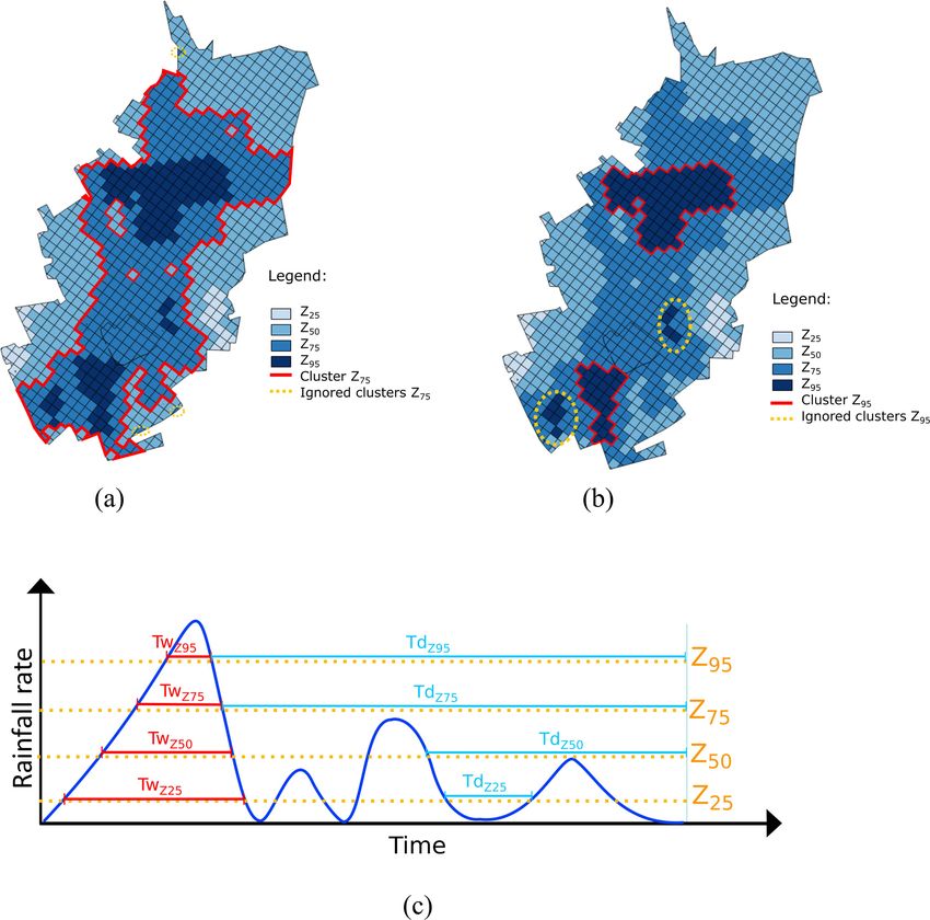
2426                                                 E. Cristiano et al.: Critical scales to explain urban hydrological response

Figure 1. Catchment area represented with the three different models: (a) SD1, (b) SD2 and (c) FD. The subdivision of the surface in sub-
catchments or two-dimensional elements is shown for each model, as well as the sewer network. The selected 13 locations and pipes are
highlighted.

tributed models, which evaluate the variability dividing the           and catchment scales, with the aim of answering the follow-
basin with a mesh of interconnected elements based on ele-             ing research questions:
vation (Zoppou, 2000; Fletcher et al., 2013; Pina et al., 2014;
Salvadore et al., 2015). Salvadore et al. (2015) analysed the            – How should rainfall variability in space and time be
most used hydrological models, comparing different model                   classified?
complexities and approaches. An investigation of the differ-             – How does small-scale rainfall variability affect hydro-
ences between high-resolution semi-distributed and fully dis-              logical response in a highly urbanized area?
tributed models was proposed by Pina et al. (2016), where
flow patterns generated with different model types were stud-            – How does model complexity affect sensitivity of model
ied and compared to observations. This work suggested that                 outcomes to rainfall variability?
although fully distributed models allow catchment variabil-
ity in space to be represented in a more realistic way, they             – How does the relationship between storm scale and
did not lead to the best modelling results because the oper-               basin scale affect hydrological response?
ation of this type of model requires very high-quality and                The paper is structured as follows. Section 2 presents the
high-resolution data, including rainfall input.                        case study, describing the study area, models and rainfall data
   Both rainfall and model resolution and scale are expected           used in this work. Methodology applied to identify variabil-
to have strong effects on hydrological response sensitivity.           ity in space and time of model and rainfall and hydrological
An increase in sensitivity is expected for small drainage areas        analysis are explained in Sect. 3. Section 4 presents the re-
and for rainfall events with high variability in space and time.       sults connected to the model and rainfall variability analysis
Sensitivity to rainfall data resolution generally increases for        and to the hydrological analysis respectively. In Sect. 5, re-
smaller urban catchments. However, sensitivity of hydrolog-            sults are discussed, by comparing the influence of rainfall and
ical models at different rainfall and catchment scales and the         model characteristics and identifying dimensionless parame-
interaction between rainfall and catchment variability need            ters to describe the relation between rainfall and model scale
a deeper investigation (Ochoa-Rodriguez et al., 2015; Pina             and rainfall resolution used. Conclusions and future steps are
et al., 2016; Cristiano et al., 2017). This work builds upon           presented in the last section.
Ochoa-Rodriguez et al. (2015), who showed that the influ-
ence of rainfall input resolution decreases with the increase
in catchment area and that the interaction between spatial and
temporal rainfall resolution is quite strong. We investigate the
sensitivity of urban hydrological response to different rainfall

Hydrol. Earth Syst. Sci., 22, 2425–2447, 2018                                        www.hydrol-earth-syst-sci.net/22/2425/2018/
E. Cristiano et al.: Critical scales to explain urban hydrological response 2427
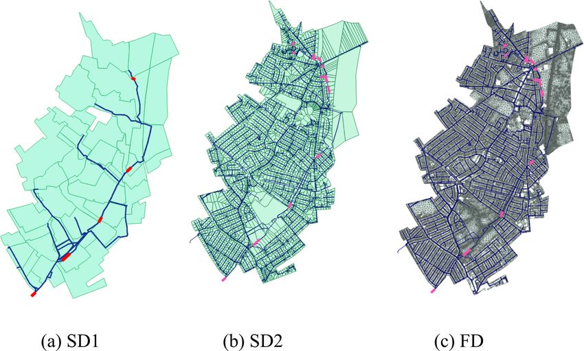
Figure 2. Illustration of rainfall cluster classification. Different colours represent different rainfall thresholds. The pixels above the same
threshold are used to estimate the percentage of coverage above a certain threshold. The red line encloses the clusters above threshold Z25
and Z95 in (a) and (b) respectively. Single isolated pixels and small clusters (yellow dotted circles) are ignored. (c) Schematic representation
of maximum wet period TwZ (red) and maximum dry period TdZ (light blue) for a pixel, for each threshold.
2 Pilot catchment and datasets Table 2 summarizes the main characteristics of the three
models: number of nodes, pipes and sub-catchments, dimen-
2.1 Study area and available models sions of sub-catchments, two-dimensional surface elements,
and degree of imperviousness. The first model, SD1, is a
The city of London (UK) is exposed to high pluvial flood low-resolution semi-distributed model, initially setup by the
risk in the last years. The Cranbrook catchment, in the Lon- water utility (Thames Water) back in 2010 to gain a strate-
don borough of Redbridge, is a densely urbanized residential gic understanding of the catchment. This model divides the
area. For this reason, it has been chosen as study area. A to- area into 51 sub-catchments, connected with 242 nodes and
tal area of approximately 860 ha is connected to the drainage 270 pipes, for a total drainage network length of just over
network, and rainfall is drained with a separate sewer system. 15 km. The other two models, SD2 and FD, have been de-
For this small catchment, several urban hydrodynami- veloped at Imperial College London (Simões et al., 2015;
cal models have been set up in InfoWorks ICM (Innovyze, Wang et al., 2015; Ochoa-Rodriguez et al., 2015; Pina et al.,
2014). Three models with different representations of surface 2016). SD2 and FD share the same sewer network design
spatial variability, are used in this study: simplified semi- (6963 nodes and 6993 pipes), but use different surface repre-
distributed low resolution (SD1), semi-distributed high reso- sentations. In SD2 the drainage area is divided into 4409 sub-
lution (SD2) and fully distributed two-dimensional high res- catchments, where rainfall runoff processes are modelled in
olution (FD). a lumped way and wherein rainfall is assumed to be uniform.
www.hydrol-earth-syst-sci.net/22/2425/2018/ Hydrol. Earth Syst. Sci., 22, 2425–2447, 2018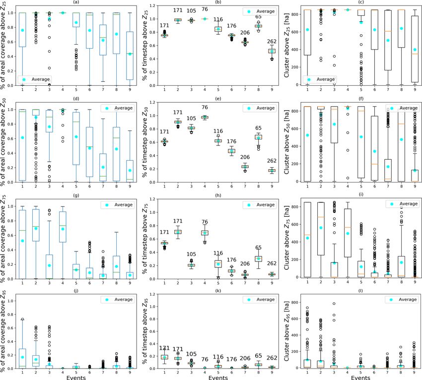
2428                                               E. Cristiano et al.: Critical scales to explain urban hydrological response

In FD, instead, the surface is modelled with a dense triangu-      3.1     Characterizing storms’ spatial and temporal
lar mesh (over 100 000 elements), based on a high-resolution               rainfall scale
(1 m × 1 m) digital terrain model (DTM). The rainfall–runoff
transformation is different for the two types of models. For       3.1.1     Spatial rainfall scale based on climatological
SD2, runoff volumes are estimated from rainfall depending                    variogram
on the land use type and routed, while for FD, runoff volumes
are estimated and applied directly on the two-dimensional el-      We computed spatial-scale characteristics based on a cli-
ements of the overland surface. Figure 1 illustrates how the       matological variogram, following the approach outlined by
surface area is modelled for each of the three models and          Ochoa-Rodriguez et al. (2015). Ochoa-Rodriguez et al.
sewer networks.                                                    (2015) presented the theoretical spatial rainfall resolution re-
                                                                   quired for an hydrological model in urban area, deriving it
2.2    Rainfall data                                               starting from a climatological (semi-) variogram. The (semi-)
                                                                   variogram γ was calculated at each time step as follows:
Cranbrook was chosen for this study because of the avail-
                                                                              n
ability of high-quality models at different spatial resolutions.            1 X
However, for this study area, only low-resolution rainfall data    γ=           (R(x) − R(x + h))2 ,                             (1)
                                                                           2n t
were available. For this reason, rainfall events measured at a
different location, with similar climatological characteristics,   where n is the number of radar pixel pairs located at a dis-
were synthetically applied over the Cranbrook catchment.           tance h, R is the rainfall rate and x is the centre of the given
Rainfall events were selected from a dataset collected by a        pixel, normalized by the sample variance and averaged over
dual polarimetric X-Band weather radar instrument located          the time period. The obtained variogram, characteristic of
in Cabauw (CAESAR weather station, NL), considering that           the averaged rainfall spatial structure during the peak pe-
the Netherlands and United Kingdom are both in the Eu-             riod, was then fitted with an exponential variogram and the
ropean temperate oceanic climate (Cfb, following the Köp-          area A under the correlogram was calculated for the expo-
                                                                                                    2
pen classification Kottek et al., 2006). For technical speci-      nential variogram as Ar = 2πr  9 . Ar can be considered as the
fications of the X-band radar device see Ochoa-Rodriguez           average area of spatial rainfall structure estimated with radar
et al. (2015). The selected events were measured with a reso-      measurements over the study area (Ochoa-Rodriguez et al.,
lution of 100 m × 100 m in space and 1 min in time, much           2015). Characteristiclength    scale rc [L] of a rainfall event
                                                                                           √
higher than what is obtained with conventional radar net-                                    2π
                                                                   was defined as rc = 3 r, where r [L] is the variogram
works (1000 m × 1000 m and 5 min). Rainfall data were ap-
plied to the Cranbrook catchment, using 16 combinations of         range. Minimum required spatial resolution 1sr was defined
space and time resolution aggregated from the 100 m–1 min          in this work as half of the storm characteristic length scale:
resolution: four spatial resolutions, 1s, (100, 500, 1000 and               rc ∼
3000 m) with four temporal resolutions, 1t, (1, 3, 5 and           1sr =       = 0.418r.                                         (2)
                                                                            2
10 min) (see Ochoa-Rodriguez et al., 2015 for a motivation of
the different resolution combinations). Nine rainfall events,         This parameter describes the spatial variability of the rain-
measured between January 2011 and May 2014, were used              fall event core.
as model input in this study. Storm characteristics are pre-
sented in Table 3.                                                 3.1.2     Rainfall spatial variability index

                                                                   Another parameter to quantify and compare the spatial vari-
3     Methods                                                      ability of rainfall is the spatial rainfall variability index Iσ .
                                                                   This parameter was at first proposed by Smith et al. (2004),
In this section, different ways of classifying spatial and tem-    called index of rainfall variability, and then recently rede-
poral rainfall scale are described, as well as some possible       fined by Lobligeois et al. (2014). This index was estimated
classification of catchment characteristics. We propose a new      as follows:
characterization of spatial and temporal rainfall variability,            P
based on the percentage of coverage above selected thresh-                   σt Rt
                                                                   Iσ = Pt         ,                                             (3)
olds. Table 1 presents the list of symbols and abbreviations                 t Rt
used in this work.
                                                                   where σt is the standard deviation of spatially distributed
                                                                   hourly rainfall across all pixels in the basin, per time step
                                                                   t, and Rt represents the spatially averaged rainfall intensity
                                                                   per time step. As can be seen, Iσ corresponds to a weighted
                                                                   average, based on instantaneous intensity, of the standard de-
                                                                   viation of the rainfall field during a given storm event. Small

Hydrol. Earth Syst. Sci., 22, 2425–2447, 2018                                     www.hydrol-earth-syst-sci.net/22/2425/2018/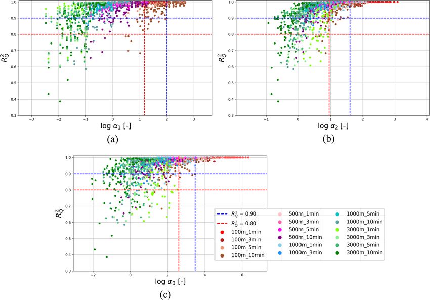
E. Cristiano et al.: Critical scales to explain urban hydrological response                                                                    2429

Table 1. List of symbols and abbreviations.

  Model characterization
  A         [L2 ]          Total catchment area                          FD                           Fully distributed model
  LC        [L]            Characteristic length of the catchment        LRA              [L]         Spatial resolution of the runoff model
  LS        [L]            Sewer length                                  SD1                          Low-resolution semi-distributed model
  SD2                      High-resolution semi-distributed model        tlag             [T]         Lag time centroid to centroid
  Rainfall resolution
  d         [T]            Rainfall event duration                       Ntot             (–)         Total number of pixels over the catchment
  1s        [L]            Spatial rainfall resolution                   1t               (min)       Temporal rainfall resolution
  Variogram
  Ar        [L2 ]          Areal average of spatial rainfall structure   n                (–)         Number of radar pixels
  R         [L T−1 ]       Rainfall rate                                 r                [L]         Variogram range
  rc        [L]            Characteristic length scale                   |v̄|             [L T−1 ]    Storm motion
  γ                        Climatological semi-variogram                 1sr              [L]         Minimum required spatial resolution
  1tr       [T]            Minimum required temporal resolution
  Spatial variability index
  Iσ        [L T−1 ]       Spatial variability index                    Rt                [L T−1 ]    Spatially averaged rainfall intensity
  σt        [L T−1 ]       Standard deviation of spatially distributed hourly rainfall
  Statistical indicators
  Pst       [L T−1 ]       Peak of aggregated rainfall                   Pref             [L T−1 ]    Measured rainfall peak (100 m–1 min)
  ReQ       (–)            Relative error on maximum flow peak           ReR              (–)         Peak attenuation ratio
   2
  RQ        (–)            Coefficient of determination for flow          2
                                                                         RR               (–)         Coefficient of determination for rainfall

  Cluster
  %cov      (–)            Percentage of coverage                      Nt               (–)      Number of pixel above Z at each time step
  SZ        [L2 ]          Cluster dimension above Z                   Z                [L T−1 ] Selected threshold
  Twmax     [T]            Maximum wet period above Z                  Tdmax            [T]      Maximum dry period above Z
  Zx        [L T−1 ]       Threshold above the xth percentile, with x ∈ [25, 50, 75, 95]
  SZx       [L2 ]          Cluster dimension above the threshold Zx , with x ∈ [25, 50, 75, 95]
  TwZx      [T]            Maximum wet period above Zx averaged over d, with x ∈ [25, 50, 75, 95]
  TdZx      [T]            Maximum dry period above Zx averaged over d, with x ∈ [25, 50, 75, 95]
  Dimensionless parameters
  S                        Subscript for spatial factors            T                                 Subscript for temporal factors
  ST                       Subscript for combined scaling factors   α1               (–)              Scaling factor that combines δS and γS
  α2        (–)            Scaling factor that combines δS and γT   α3               (–)              Scaling factor that combines δST and γST
  δ         (–)            Rainfall scaling factor using SZ75       γ                (–)              Model scaling factor
  θ         (–)            Scaling factors proposed by Ochoa-Rodriguez et al. (2015)

values of Iσ indicate a low rainfall variability, typical of strat-             3.1.3    Storm motion velocity and temporal rainfall
iform rainfall events. Large values of Iσ generally represent                            variability based on storm cell tracking
convective storms, characterized by high spatial variability.
In the study presented by Lobligeois et al. (2014), Iσ was                      Ochoa-Rodriguez et al. (2015) presented a characterization
applied to rainfall data measured in a French region with a                     of storm motion and a definition of the minimum required
resolution of 1000 m–5 min and it varied between 0 and 5.                       temporal resolution. Storm motion was defined applying the
                                                                                TREC method (TRacking Radar Echoes by Correlation) pro-
                                                                                posed by Rinehart and Garvey (1978) This method allows
                                                                                a vector representing storm motion velocity magnitude and
                                                                                direction of the rainfall event to be obtained at each time
                                                                                step. The minimum required temporal resolution, 1tr , was

www.hydrol-earth-syst-sci.net/22/2425/2018/                                                     Hydrol. Earth Syst. Sci., 22, 2425–2447, 2018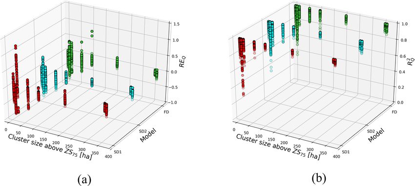
2430                                                    E. Cristiano et al.: Critical scales to explain urban hydrological response

Figure 3. Percentage of areal coverage above selected threshold, calculated over all time steps and per rainfall event (a, d, g, j). Temporal
percentage of coverage above the selected threshold, defined as number of time steps above the threshold at each pixel, divided by the total
duration of the event (b, e, h, k). Temporal percentage is presented for each rainfall event and the number above each box plot indicates the
total duration of the rainfall event. Cluster dimensions across all time steps per event for the four selected thresholds (c, f, i, l). Blue dots
represent the average, green or red lines the median, boxes indicate the first to third quartile, and whiskers extend 1.5 times the interquartile
range below the first and above the third quartile.

obtained considering time that a storm needs to pass over the              storm motion velocity vectors, estimated at each time step
storm event characteristic length scale rc . The term 1tr can              during the peak period.
be written as follows:
                                                                           3.1.4    Rainfall spatial scale based on fractional
       rc                                                                           coverage of basin by storm core
1tr =      ,                                                      (4)
      |v̄|
                                                                           In this work, a different approach to classify rainfall events is
where |v̄| [L T−1 ] corresponds to the mean storm motion ve-               presented, considering storm spatial and temporal variability
locity magnitude, and |v̄| is obtained from the average of the             in combination with rainfall intensity thresholds. To select

Hydrol. Earth Syst. Sci., 22, 2425–2447, 2018                                             www.hydrol-earth-syst-sci.net/22/2425/2018/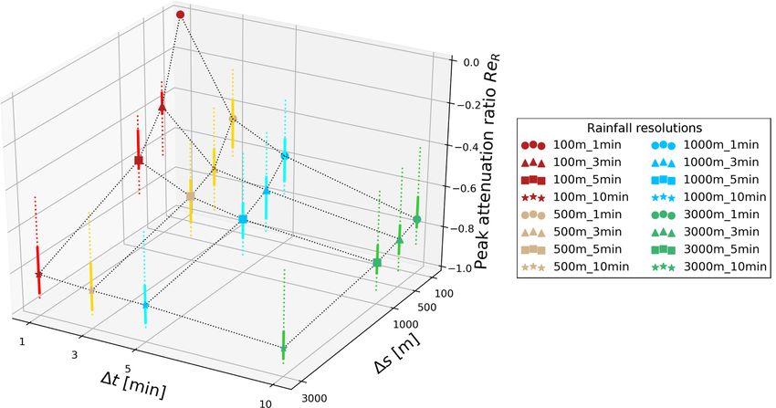
E. Cristiano et al.: Critical scales to explain urban hydrological response                                                           2431

Table 2. (a) Summary of the hydrological model characteristics of
the three models. (b) Drainage area connected to the investigated                P
locations for each model.                                                            t Nt
                                                                       %cov =               .                                           (5)
                                                                                 Ntot · d
     (a)
                                                                          The percentage of coverage was calculated for each event,
                                       SD1           SD2         FD    in order to give a first classification of the spatial rainfall vari-
     No. of sub-catchments               51         4409       4367    ability.
     No. of nodes                       242         6963       6963
     No. of pipes                       270         6993       6993    3.1.5   Rainfall cluster classification
     Catchment area (ha)                846           851       851    Since variograms provide a strongly smoothed measure of
     Contributing % impervious           43            40        15    rainfall field, we used alternative metrics to characterize the
     Contributing % pervious             56            60         0
                                                                       space scale and timescale of storm events based on cluster
     Average area (ha)                 16.6           0.2    0.006*    identification. To analyse the spatial variability of the storm
     Standard deviation (ha)           13.4            0.8   0.000*    core, we identified, for each rainfall event, the main rainfall
     Max. (ha)                         61.8          40.1    0.099*    cluster dimension SZ above the selected thresholds Z, as de-
     Min. (ha)                         11.7         0.005    0.006*    fined in Sect. 3.1.4.
     Total length (km)                 ∼ 16     ∼ 150         ∼ 150       For each time step, the area covered by rainfall above a cer-
     No. of manholes                    236      6207          6207    tain threshold was considered. Main clusters were defined as
     No. of 2-D elements                 no        no        117 712   the union of rainfall pixels above a given threshold. To iden-
                                                                       tify the clusters, an algorithm based on Cristiano and Gaitan
                (b)
                                                                       (2017) has been used. The algorithm executes the following
                            SD1        SD2           FD                rules:
                            (ha)       (ha)         (ha)
                                                                         – All pixels above a certain threshold are considered.
                Loc1           –       0.9        0.9
                Loc2           –       6.7        6.6                    – A pixel is included in the cluster if at least one of its
                Loc3           –       9.5        9.5                      boundaries borders the cluster.
                Loc4           –      21.3       21.3
                Loc5           –      24.6       24.6                    – Small clusters, with an area smaller than 9 ha (about 1 %
                Loc6          36      42.9       42.9                      of catchment area) are ignored.
                Loc7          80      43.7       43.7
                Loc8          80      83.9       83.9                    – In the case of more than one cluster, the average of clus-
                Loc9         137     129.2      129.2                      ter areas is considered, in order to compare the cluster
                Loc10        290     254.8      254.8                      size at different time steps. This happens in only a few
                Loc11        484     448.3      448.3                      cases.
                Loc12        538     502.5      502.5
                Loc13        846     626.6      626.6                     To obtain a characteristic number for each storm, cluster
               * Dimension of the two-dimensional
                                                                       sizes per time step were averaged over the entire duration of
               triangular mesh elements.                               rainfall event. Figure 2 presents an example of rainfall cov-
                                                                       erage at a time step t. Rainfall was divided considering dif-
                                                                       ferent thresholds and the red line highlights the cluster for
the thresholds Z for the nine rainfall events over the radar           Z75 in Fig. 2a and for Z95 in Fig. 2b. The clusters identified
grid (6 km × 6 km), percentiles at 25, 50, 75 and 95 % of              with yellow circles are ignored because they are too small to
the entire 100 m–1 min resolution rainfall dataset were cal-           give a considerable contribution. In a case in which there is
culated. In this way it was possible to calculate the different        more than one cluster, as for Fig. 2b, the average of the main
thresholds Z25 , Z50 , Z75 and Z95 , corresponding to the 25th,        clusters is considered.
50th, 75th and 95th percentiles.
   Fractional coverage was largely studied in the literature           3.1.6   Maximum wetness period above rainfall
and it was shown that it has a strong influence on flood re-                   threshold
sponse (Syed et al., 2003; ten Veldhuis and Schleiss, 2017).
The percentage of coverage %cov used in this study, was de-            To identify the characteristic timescale of rainfall events,
fined as the sum of the number of pixels Nt above a threshold          maximum wetness periods were defined as the number of
at each time step t divided over the total number of pixels of         time steps estimated for which rainfall at a pixel is constantly
the catchment Ntot and over the total number of time steps d           above a given threshold. With this aim, every pixel in the
of the event:                                                          catchment was analysed and maximum number of consec-
                                                                       utive time steps above the chosen threshold was retrieved.

www.hydrol-earth-syst-sci.net/22/2425/2018/                                          Hydrol. Earth Syst. Sci., 22, 2425–2447, 2018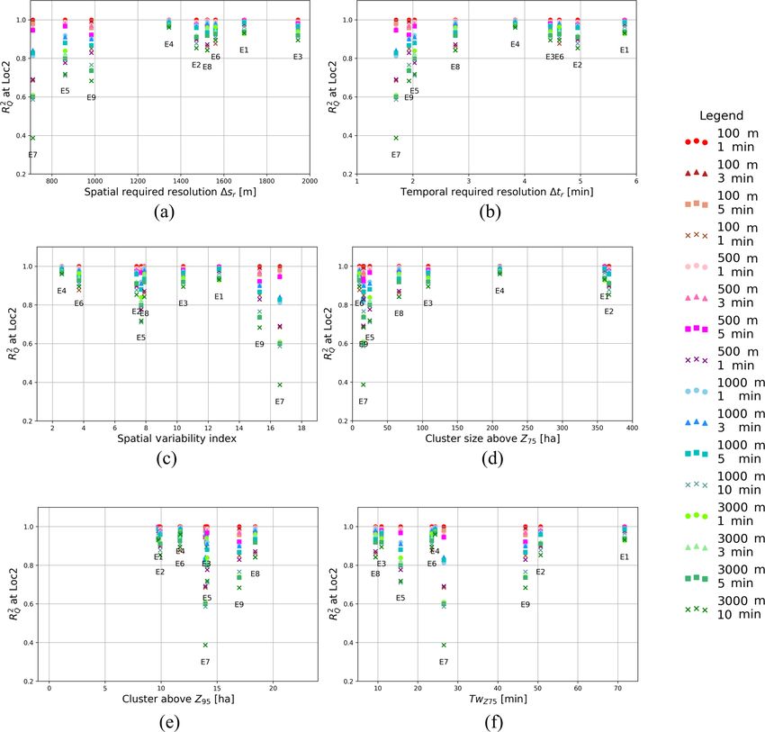
2432                                                      E. Cristiano et al.: Critical scales to explain urban hydrological response

Table 3. Rainfall event characteristics.

                    Event    Date                          Initial–   Total depth (areal average/   Max intensity over 1 min
                    ID                                ending times          pixel min/pixel max)              (areal average/
                                                                                           (mm)             individual pixel)
                                                                                                                   (mm h−1 )
                    E1       18 January 2011          05:10–08:00                      31/18/46                     32/1120
                    E2       18 January 2011          05:10–08:00                      36/16/47                      26/124
                    E3       28 June 2011             22:05–23:55                        9/4/18                      28/242
                    E4       18 June 2012             05:55–07:10                       10/8/12                       12/24
                    E5       29 October 2012          17:05–19:00                        5/1/14                        7/83
                    E6       2 December 2012          00:05–03:00                         5/2/8                        7/39
                    E7       23 June 2013             08:05–11:30                        4/1/13                       9/307
                    E8       9 May 2014               18:15–19:35                         4/1/9                       13/67
                    E9       11 May 2014              19:05–23:55                        6/1/13                      11/247

Figure 2c illustrates the process followed to select the max-                ered. Given that the coarser resolution model (SD1) does not
imum duration Twmax above the threshold Z. For each pixel,                   contain small drainage areas (< 35 ha), only 8 of the 13 se-
the value of the maximum duration above the threshold is                     lected locations were available for SD1. To compare FD with
identified. These values are averaged over the whole catch-                  SD models, we assumed that FD sub-catchments have the
ment to obtain a temporal length scale that characterizes rain-              same dimension of SD2 sub-catchments. Table 2b presents
fall event TwZ .                                                             the drainage area Ad connected to each location, while in
   For each pixel n, the maximum wetness period TwZ above                    Fig. 1 the location of the selected pipes is highlighted on the
                                           NP
                                            tot
                                                  Twmax
                                                                             catchment with a thick red line.
a selected threshold Z is defined as nP N , where Ntot is                       Dimensionless parameters as proposed by Bruni et al.
                                             tot
the total number of pixels.                                                  (2015) and Ogden and Julien (1994) were determined to in-
   In order to characterize the intermittency of rainfall events,            vestigate the interaction and relation between rainfall resolu-
the maximum dry period Tdmax , defined as the maximum                        tion and different model properties and characteristics. The
                                                                                                              1s
number of time steps during which the threshold Z was not                    catchment sampling number L       C
                                                                                                                  was introduced as the ra-
exceeded, was also identified. Figure 2c shows how these                     tio of the rainfall spatial resolution 1s to the characteristic
lengths, TwZ and TdZ , were selected. The combination of                     length of the catchment LC (square root of the total area).
these two parameters gives an indication of how constant or                  This parameter describes the interaction between rainfall res-
intermittent is the rainfall event.                                          olution and study area. If the catchment sampling number
                                                                             is higher than 1, rainfall variability is insufficiently captured
3.2     Characterizing hydrological models’ spatial and                      and for small rainfall events the position might not be prop-
        temporal scales                                                      erly represented. The runoff sampling number was defined
                                                                             as L1s
                                                                                  RA
                                                                                     , where LRA indicates the spatial resolution of the
3.2.1    Models’ spatial scales                                              runoff model, defined as the square root of the averaged sub-
                                                                             catchment size (Bruni et al., 2015). Lower values of this ratio
Several studies have shown that drainage area is one of the                  indicate that the model is unable to capture rainfall variabil-
dominating factors affecting the variation in urban hydrolog-                ity, while higher values indicate possible incorrect transfor-
ical responses resulting from using rainfall at different spa-               mation of rainfall into runoff. The sewer sampling number
                                                                             1s
tial and temporal resolutions as input (Berne et al., 2004;                   LS describes the interaction between rainfall resolution and
Ochoa-Rodriguez et al., 2015; Yang et al., 2016). Consider-                  sewer length LS , indicating higher sensitivity to rainfall vari-
ing a larger drainage area implies aggregating and averaging                 ability with increasing values of this ratio.
rainfall and consequently smoothing rainfall peaks, with the
result of having large areas that are less sensitive to high-                3.2.2   Models’ temporal scales
resolution measurements.
   In order to compare spatial scale of models and rainfall                  In the literature, there is no unique parameter to character-
spatial variability, the average dimension of sub-catchments                 ize the temporal variability of the model. Several authors
was analysed to characterize the model spatial scales. To in-                have proposed different timescale characteristics (see Cris-
vestigate the effects of the drainage area Ad on hydrological                tiano et al., 2017 for a review), but no unique formulation
response sensitivity, 13 locations, with connected surface that              has been chosen yet, especially for urban areas. Time of
varies from less than 1 ha to more than 600 ha, were consid-                 concentration (McCuen et al., 1984; Singh, 1997; Musy and

Hydrol. Earth Syst. Sci., 22, 2425–2447, 2018                                               www.hydrol-earth-syst-sci.net/22/2425/2018/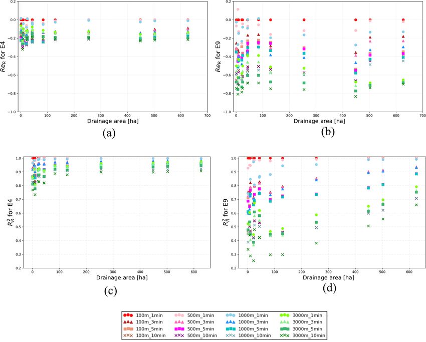
E. Cristiano et al.: Critical scales to explain urban hydrological response                                                                 2433

Figure 4. Variability of the lag time, depending on the location, for each model (a). The box plots represent the median (red line), the upper
(third quartile) and lower (first quartile) quartile (boxes boundaries), and 1.5 times the interquartile range below the first and above the third
quartile (whiskers). Drainage areas corresponding to each location are presented in Table 2b. Average, median, minimum and maximum
value of the lag time as a function of Ad for SD2. (b) Fitting power law curves and the power law relation proposed by Berne et al. (2004)
are plotted.

Higy, 2010) and lag time (Berne et al., 2004; Marchi et al.,               sub-catchment, while the hydrograph was represented using
2010) are the most commonly used temporal model scales,                    the flow in selected pipes. The lag time can be considered as
but other time lengths have been proposed in the literature                a characteristic basin element. It depends on drainage area
(Ogden et al., 1995; Morin et al., 2001). In this study, tem-              size, slope and imperviousness (Gericke and Smithers, 2014;
poral variability of the three models was classified using lag             Morin et al., 2001; Berne et al., 2004; Yao et al., 2016), but it
time tlag , which describes the runoff delay compared to rain-             is also influenced by rainfall characteristics. For this reason,
fall input. The variable tlag can be defined in different ways:            tlag was calculated for the nine rainfall events and the average
as the difference between the centroid of the hyetograph and               of these values was taken as the representative number.
the centroid of the hydrograph (Berne et al., 2004), or as the                Lag time increases with drainage area, following a power
distance between rainfall and flow peaks (Marchi et al., 2010;             law as proposed by Berne et al. (2004). For urban areas, an
Yao et al., 2016). The hyetograph in a specific location was               empirical relation between catchment area A (ha) and lag
estimated as the average of rainfall intensity in the considered           time tlag (min) was presented:

www.hydrol-earth-syst-sci.net/22/2425/2018/                                               Hydrol. Earth Syst. Sci., 22, 2425–2447, 2018
2434                                                   E. Cristiano et al.: Critical scales to explain urban hydrological response

Figure 5. Peak attenuation ratio ReR for the nine rainfall events, as a function of temporal and spatial rainfall resolution. Symbols indicate
the median over the nine events, solid lines represent the first to the third quartile, dotted lines vary from minimum to maximum. Colours
represent different temporal resolutions and markers used for the median indicate different spatial resolutions.

Table 4. Rainfall spatial and temporal characterization proposed by Ochoa-Rodriguez et al. (2015) and rainfall spatial variability index
proposed by Lobligeois et al. (2014).

                                      Ochoa-Rodriguez et al. (2015)                          Lobligeois et al. (2014)
                   Event    Spatial          Mean       Required       Required      Spatial variability   Spatial variability
                   ID        range    storm motion        spatial     temporal r                  index                 index
                                           velocity    resolution     resolution       at 100 m–1 min       at 1000 m–5 min
                                (r)           (|v̄|)         1sr            1tr                      Iσ             Iσ 1000 m
                               (m)         (m s−1 )          (m)          (min)              (mm h−1 )             (mm h−1 )
                   E1         4057               9.8        1695            5.8                     12.7                  6.4
                   E2         3525               9.9        1473            5.0                      7.4                  5.2
                   E3         4655              14.0        1945            4.6                     10.4                  6.5
                   E4         3219              11.7        1345            3.8                      2.6                  1.5
                   E5         2062              14.1         861            2.0                      7.7                  4.2
                   E6         3738              11.7        1561            4.5                      3.7                  2.0
                   E7         1703              14.0         711            1.7                     16.6                  5.9
                   E8         3644              18.4        1523            2.8                      7.9                  4.2
                   E9         2355              17.0         984            1.9                     15.3                  6.5

                                                                          3.3      Statistical indicator for analysing rainfall
                                                                                   sensitivity
tlag = 3A0.3 .                                                  (6)
                                                                          To investigate the effects of rainfall aggregation on peak
   This relation was confirmed, incorporating results ob-                 intensity, the peak attenuation ratio ReR was calculated
tained by Schaake and Knapp (1967) and Morin et al. (2001).               for rainfall. This parameter represents peak underestimation
tlag was calculated for each selected sub-catchment, and then             when aggregating in space and time and it was defined as
compared with the rainfall temporal scale, to investigate the             follows:
interaction between model and rainfall scale. The relation be-
tween averaged lag time and connected drainage area was                              Pst − Pref
studied at each location.                                                 ReR =                 ,                                         (7)
                                                                                        Pst

                                                                          where Pref is the peak of the measured rainfall at 100 m–
                                                                          1 min resolution and Pst is the rainfall peak at the aggregated

Hydrol. Earth Syst. Sci., 22, 2425–2447, 2018                                              www.hydrol-earth-syst-sci.net/22/2425/2018/
E. Cristiano et al.: Critical scales to explain urban hydrological response 2435
Figure 6. Impact of aggregation in space and time on rainfall peak (ReR ) and overall pattern (RR 2 ) for two selected events, as a function of
sub-catchment size (Ad ). E4 is a constant low-intensity event with low spatial variability. E9 is an example of an intermittent event, with a
high storm motion velocity. Different colours and symbols indicate different rainfall resolutions used as input. Other events are presented in
the Supplement.
resolution s in space and t in time. ReR values vary from 0 3.4 Statistical indicators for analysing hydrological
to 1, a condition for which there is no underestimation. response
The coefficient of determination RR2 was used to describe
rainfall intensity sensitivity to aggregation in space and time. Rainfall was synthetically applied over models and flow and
RR2 represents the portion of variance of dependent variables depth were calculated in 13 selected locations, to study the
that is predictable from the independent one. This parameter hydrological response and to compare the three models. Fol-
indicates how well regression approximates real data points. lowing Ochoa-Rodriguez et al. (2015), rainfall was applied in
RR2 values can vary between 1 and 0, where 1 represents the such a way that the storm movement main direction was par-
perfect match between observed rainfall values Rref and the allel to the main downstream direction of flow in pipes. The
aggregated value Rst at spatial resolution s and temporal res- rainfall grid centroid coincided with the catchment centroid.
olution t. Using aggregated rainfall data as input and hydrodynamic
simulation results derived from the highest-resolution rain-
fall (100 m and 1 min) as reference, the following two statis-
tical indicators were calculated and analysed to quantify the
influence of rainfall input resolution, at selected locations.
www.hydrol-earth-syst-sci.net/22/2425/2018/ Hydrol. Earth Syst. Sci., 22, 2425–2447, 20182436 E. Cristiano et al.: Critical scales to explain urban hydrological response
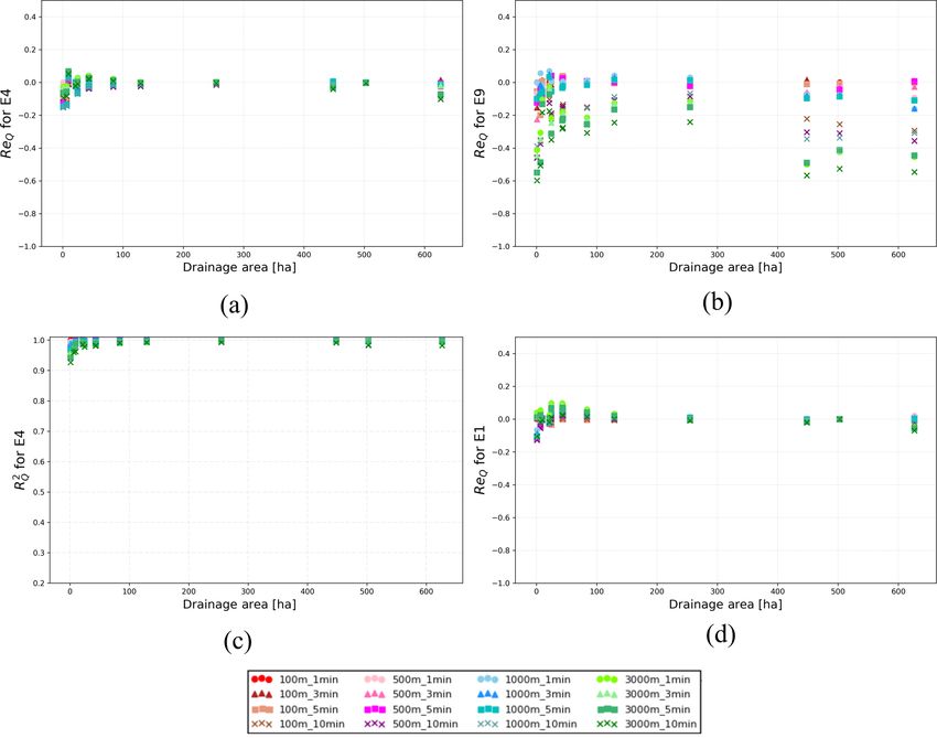
Figure 7. Relative error in peak ReQ and coefficient of determination RQ 2 for SD2, plotted as a function of A , for the 16 combinations of
d
rainfall input resolutions. Two different events are presented: E4, a low-intensity constant event, and E9, a multiple-peak event.
– Relative error in peak flow ReQ : 3.5 Scaling factors characterizing rainfall and model
Qmaxst −Qmaxref scales
ReQst = Qmaxref where Rest is the relative error
in peak (Qmaxst ) corresponding to a rainfall input of spa-
tial resolution s and temporal resolution t, in relation to To investigate the impact of spatial and temporal scales of
the reference (100 m–1 min) flow peak, Qmaxref (Ochoa- rainfall events on the sensitivity of simulated runoff to differ-
Rodriguez et al., 2015). Rest values bigger than zero ent rainfall input resolutions, Ochoa-Rodriguez et al. (2015)
indicate an overestimation of the peak associated with defined spatial and temporal scaling factors, θS and θT . These
the rainfall input st, and, vice versa, Rest values smaller factors were defined as the ratio between required spatial
than zero indicate an underestimation. and temporal minimum resolutions, 1sr and 1tr , and spa-
2: tial and temporal resolutions considered as input 1s and 1t:
– Coefficient of determination RQ θS = 1s r 1tr
2 , as described in Sect. 3.3 for rainfall, was also ap- 1s and θT = 1t . The combined effects of spatial and
RQ temporal characteristics were evaluated, defining a combined
plied to the flow, to investigate effects of rainfall aggre- spatial–temporal factor which accounts for spatial–temporal
gation on hydrological response. scaling anisotropy factor Ht (Ochoa-Rodriguez et al., 2015).
The anisotropy factor represents the relation between spatial
and temporal scales, assuming that atmospheric properties
and Kolgomorov’s theory (Kolgomorov, 1962) are also valid
for rainfall (Marsan et al., 1996; Deidda, 2000; Gires et al.,
Hydrol. Earth Syst. Sci., 22, 2425–2447, 2018 www.hydrol-earth-syst-sci.net/22/2425/2018/E. Cristiano et al.: Critical scales to explain urban hydrological response 2437
2011). Combined spatial–temporal factor is then defined as A second possible way to combine rainfall and model
1
1−Ht characteristics was α2 :
follows: θST = θS ·θT , where Ht usually assumes the value
√
of one-third (Marsan et al., 1996; Gires et al., 2011, 2012). SZ75 tlag
Building on the work of Ochoa-Rodriguez et al. (2015), α2 = · = δS · γT . (15)
1s 1t
we proposed spatial and temporal scaling rainfall factors, δS
and δT . Rainfall cluster classification and maximum wetness In this case, both spatial and temporal aspects were consid-
period were used to describe the rainfall scale. The 75th per- ered. The catchment temporal scaling factor represents both
centile threshold was chosen as reference, according to the spatial and temporal variability of the catchment, because of
results presented in Sect. 4.4.3. The rainfall factors are de- the strong relationship between lag time and drainage area
fined as the ratio of cluster dimension SZ75 above Z75 to described in Sect. 3.2.2.
maximum wetness period TwZ75 above Z75 and spatial and The third scaling factor, α3 , combines all spatial and tem-
temporal rainfall resolutions: poral rainfall and model characteristics. The term α3 was de-
fined as follows:
√ √
SZ75 SZ75 · Ad TwZ75 · tlag
δS = , (8) α3 = · = δST · γST . (16)
1s 1s 2 1t 2
Tw
δT = Z75 . (9) These parameters allow the best rainfall resolution or
1t model scale to be chosen. Depending on the available data
The characteristic spatial length of the main cluster, corre- and on the level of performance that we want to achieve, it is
sponding to the square root of the main cluster, was used to possible to identify the required rainfall resolution.
define the spatial rainfall scaling factor. Combined effects of
spatial and temporal rainfall scale were investigated, defining
4 Results and discussion
δST as a combination of δS and δT .
4.1 Rainfall analysis
δST = δS · δT (10)
In this section, methods for quantifying rainfall space and
The coefficient of anisotropy was not considered for the new timescales proposed in the literature (Ochoa-Rodriguez et al.,
parameters. The assumption that the anisotropy observed in 2015; Lobligeois et al., 2014) are compared to the cluster
the atmosphere is also present in the hydrological response classification we propose in this paper. Additionally, change
is not always applicable. Results were, however, investigated in rainfall characteristics with spatial and temporal aggrega-
with and without the anisotropy and no big differences were tion scale will be analysed.
identified.
A similar concept was applied to model characteristics, 4.1.1 Spatial and temporal classification results
and spatial and temporal model scaling factors were defined.
These factors were obtained, comparing model characteris- Spatial variability index values for each of the nine rain-
tic length (square root of drainage area Ad ) and lag time tlag fall events are presented in Table 4 for the observed rain-
with spatial and temporal resolution respectively. fall at 100 m–1 min (Iσ ) and at 1000 m–5 min (Iσ 1000 m ). The
√ last two columns on the right were added to have a direct
Ad comparison with the values presented by Lobligeois et al.
γS = (11)
1s (2014), who used the same resolution. Iσ values are gen-
tlag erally high when compared to values found by Lobligeois
γT = (12)
1t et al. (2014) for all the investigated regions. This indicates
that most events are characterized by high spatial variability.
The combined model scaling factor was defined as fol- Aggregation has a strong impact on this parameter, which
lows: becomes smaller with a coarser resolution, highlighting the
fact that information about rainfall variability is lost during
γST = γS · γT . (13)
the coarsening process. Iσ 1000 m values are generally higher
With the aim to identify a factor that represents the be- than values presented for the northern region, where values
haviour of hydrological response sensitivity well, three new are below 1, but are comparable to the Mediterranean area,
parameters are presented. The first factor is α1 , which ac- where Iσ reaches values around 4.
counts only for the spatial aspects of model and rainfall vari- Values obtained based on variogram analysis (spatial
ability. The term α1 was defined as follows: range) and storm tracking (temporal development) following
Ochoa-Rodriguez et al. (2015) are also presented in Table 4.
√ Results show that the spatial variability index tends to in-
SZ75 · Ad
α1 = . (14) crease as well as the required spatial resolution for storms
1s 2
www.hydrol-earth-syst-sci.net/22/2425/2018/ Hydrol. Earth Syst. Sci., 22, 2425–2447, 20182438 E. Cristiano et al.: Critical scales to explain urban hydrological response
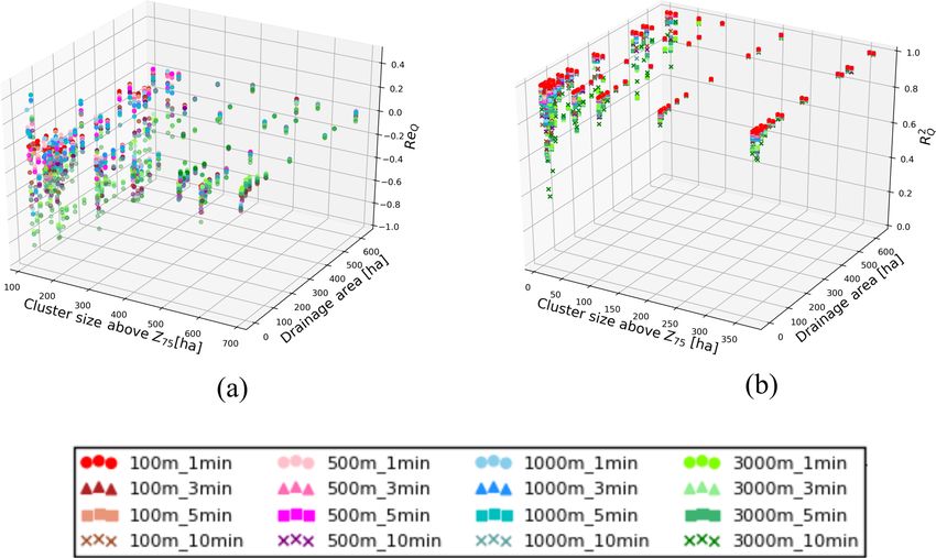
Figure 8. ReQ and RQ 2 variability, in relation to model type and rainfall characterized by cluster dimension S
Z75 , for all locations and all
combinations of rainfall input resolution. Colours identify the three different models.
Table 5. Thresholds values obtained for the nine rainfall events con- and E7, the 25 mm h−1 threshold is exceeded over a 15 min
sidered. time window, for few time steps and, in particular, for E7 this
happens only at the peak. This implies that rainfall events
Threshold Z25 Z50 Z75 Z95 considered in this study are not classifiable as extreme.
Percentile 25 % 50 % 75 % 95 % The percentage of areal coverage, estimated for the catch-
Values 0 mm h−1 0.5 mm h−1 7 mm h−1 22 mm h−1 ment, is presented in Fig. 3a, d, g, j. Areal coverage as-
sociated with 25th percentile values provides an indication
of event-scale intermittency. Events with 25th percentiles
larger than 2500 m spatial range, while events with small spa- close to 1 cover the entire catchment most of the time, while
tial range (E5, E7 and E9, spatial range below 2500 m) are smaller and more intermittent events, especially E7 and E9,
characterized by relatively high spatial variability indexes. are characterized by lower 25th percentile values. Areal cov-
Required temporal resolution 1tr , obtained from the com- erage for 95th percentile thresholds indicates the size of
bination of storm motion velocity and required spatial reso- storm cell cores: E1 and E2 have storm cores covering up
lution (see Sect. 3.1.3) varies between 1.7 and 5.9 min; the to 65–70 % of the catchment; E4 and E6 have median cover-
lowest values of 1tr are associated with fast storm events age values close to zero, indicating that these are mild events
(e.g. E8 and E5) and small-scale events (e.g. E9 and E7). without an intense storm core.
Box plots in Fig. 3b, e, h and k show the number of time
4.1.2 Thresholds and percentage of coverage steps above selected thresholds as a percentage of total event
duration, to enable comparison between events. Results con-
The first step in obtaining cluster dimensions is to identify firm patterns identified based on areal coverage: events E7
rainfall thresholds (Z) characterizing the rainfall values’ dis- and E9 are identified as high-intermittency events (based
tribution (see Sect. 3.1.4). Table 5 shows rainfall threshold on 25th percentile threshold). Maximum percentage of time
values corresponding to the 25th, 50th, 75th and 90th per- steps above the highest threshold is 30 % for events E1 and
centiles for the nine rainfall events. E2. Each box plot represents the spatial variability of rain-
The 25th percentile of the rainfall values distribution is fall between pixels. Thresholds Z50 and Z75 present a high
zero, indicative of strong intermittency and small areal cover- intra-event variability, highlighting the differences between
age of some of the events (especially events E7 and E9). The rainfall events. For the other two thresholds, the intra-event
95th percentile is 22 mm h−1 (over a 1 min time window), variability is not high, suggesting that the rainfall event char-
corresponding to a recurrence interval of less than 6 months acteristics might not be well represented. For Z95 , all events
(KNMI, 2011), indicating that the selected events are repre- present a coverage variability lower than 30 %, and differ-
sentative of frequently occurring events. For this region, rain- ences between events are not properly defined. Thresholds
fall intensities above 25 mm h−1 , over a 15 min time window, Z50 and Z75 present also a high inter-event variability, indi-
correspond to a return period of once per year, indicating an cating that in these cases the spatial variability of the rainfall
intense rainfall event. For only few rainfall events, E1, E2, E3 event above the catchment area is high.
Hydrol. Earth Syst. Sci., 22, 2425–2447, 2018 www.hydrol-earth-syst-sci.net/22/2425/2018/E. Cristiano et al.: Critical scales to explain urban hydrological response 2439
Figure 9. RQ2 at Loc2 for different rainfall resolution, plotted against different rainfall characterizing scales: spatial (a) and temporal (b) re-
quired resolution, spatial variability index (c), dimension of cluster above Z75 (d) and Z95 (e), and maximum wet period above Z75 (f).
4.1.3 Rainfall cluster classification shape during the event. Only a couple of events, E4 and E2,
do not show high variability above Z25 and Z50 threshold.
For Z95 , the cluster dimension variability is relatively small,
Dimensions of the main cluster were determined for each of suggesting that the average or the median can be a good ap-
the four thresholds and for all time steps of the nine events. proximation of the storm core dimension. Values above Z50
Results are presented in Fig. 3c, f, i and l, where the red line present high inter-event variability. There is a clear distinc-
indicates the median and the blue dot the average. tion between constant events, such as E2 and E4, and inter-
The plots show that for Z25 only intermittent events, like mittent events, E7 and E9, which show low median and av-
E7 and E9, present a median below 861 ha (entire catch- erage values.
ment area). The intra-event variability is generally quite high Intense and constant rainfall events are also character-
for most of the events, especially for the 50th and 75th per- ized by median values being generally higher than the mean.
centiles, indicating that clusters change their dimension and
www.hydrol-earth-syst-sci.net/22/2425/2018/ Hydrol. Earth Syst. Sci., 22, 2425–2447, 20182440 E. Cristiano et al.: Critical scales to explain urban hydrological response
Table 6. Maximum wetness periods above the threshold, calculated for each pixel, averaged over the total catchment, and then divided by
the total duration.
Maximum wet period Maximum dry period
Event ID TwZ25 TwZ50 TwZ75 TwZ95 TdZ25 TdZ50 TdZ75 TdZ95
(–) (–) (–) (–) (–) (–) (–) (–)
E1 0.53 0.50 0.42 0.17 0.16 0.25 0.27 0.35
E2 0.98 0.74 0.30 0.06 0.02 0.07 0.13 0.30
E3 0.97 0.43 0.10 0.06 0.02 0.08 0.63 0.72
E4 1.00 0.98 0.32 0.01 0.01 0.02 0.11 1.00
E5 0.77 0.57 0.14 0.11 0.11 0.28 0.38 0.57
E6 0.52 0.24 0.13 0.12 0.12 0.29 0.52 0.99
E7 0.28 0.14 0.13 0.12 0.13 0.28 0.53 0.71
E8 0.83 0.43 0.14 0.07 0.07 0.22 0.34 0.53
E9 0.22 0.19 0.18 0.17 0.17 0.30 0.56 0.69
Table 7. Dimensionless parameters for the three models used in this study, based on Bruni et al. (2015), used to describe the interaction
between spatial rainfall resolution and model scale.
Catchment sampling Runoff sampling Sewer sampling
number number number
1s SD1 SD2 FD SD1 SD2 FD SD1 SD2 FD
100 m 0.03 0.04 0.04 0.25 2.29 10 0.19 1.73 1.73
500 m 0.17 0.20 0.20 1.23 11.47 50 0.94 8.65 8.65
1000 m 0.34 0.40 0.40 2.45 22.94 100 1.87 17.30 17.30
3000 m 1.03 1.20 1.20 7.35 68.82 300 5.62 51.91 51.91
However, intermittent events, such as E9, have an average old (E4, E3). E7 and E9 present a moderate decrease in TwZ
higher than the median, especially for the 50th and 75th per- while they have a steep increase in TdZ , indicative of strong
centiles. These results suggest that Z50 and Z75 are able to intermittency. For the other events, the behaviour is generally
describe rainfall spatial and temporal scale well. the opposite, indicative of a concentrated storm core.
4.1.4 Maximum wet and dry period 4.2 Hydrological model, spatial and temporal scales
The maximum wet period TwZ and maximum dry period TdZ 4.2.1 Spatial model scale
were calculated for four rainfall intensity thresholds in order
to represent temporal variability of a rainfall event. Table 6 Dimensionless sampling numbers, presented at first by Og-
presents maximum wetness period TwZ and maximum dry den and Julien (1994), and then re-proposed by Bruni et al.
period TdZ , normalized by total duration of the rainfall event, (2015), are presented in Table 7 for the three models (for
to enable comparison between events and to investigate how underlying equations see Sect. 3.2.1). SD2 and FD model
long the main core is in relation to the total duration of the have the same contributing area and network length, hence
event. they show that values for the catchment sampling number
For some events TwZ decreases depending on the thresh- and sewer sampling number are the same.
old, passing from values close to 1 for Z25 to values close Catchment sampling numbers higher than 1 indicate that
to 0 for Z95 . The change between different thresholds can be models can not properly represent rainfall variability (Bruni
gradual, as for example for E2, E8 or E5, or sharp, as is the et al., 2015). In this study, for 3000 m spatial rainfall reso-
case of E3 or E4. For intermittent events, however, the max- lution values are bigger than 1, so poor model performance
imum wet period does not vary too much, and it is relatively at this resolution is expected. The runoff sampling number
short, like E7 or E9. This implies that there are probably mul- suggests that SD1 will not be able to capture rainfall variabil-
tiple short periods above the threshold. When comparing TwZ ity, because it presents low values for all spatial resolutions,
and TdZ , we can observe that some events show a symmetri- while FD has high values of this parameter, which highlights
cal behaviour, when a decrease in wet period coincides with some uncertainty in rainfall–runoff transformation. SD2, in-
an increase in dry period, with the increase in the thresh- stead, presents runoff sampling numbers similar to the values
Hydrol. Earth Syst. Sci., 22, 2425–2447, 2018 www.hydrol-earth-syst-sci.net/22/2425/2018/E. Cristiano et al.: Critical scales to explain urban hydrological response 2441
2 as a function of cluster dimension above Z and A . Different colours and symbols indicates different rainfall
Figure 10. ReQ and RQ 75 d
resolution input.
found by Bruni et al. (2015), where this parameter varied be- 4.2.2 Temporal model scale
tween 2.6 for high resolution and 93 for lower resolution.
The sewer sampling number applied to SD2 and FD presents Lag time tlag was computed for 9 storms for each model at
similar results to Bruni et al. (2015), where the values were 12 sub-catchments and at the catchment outlet, as explained
varying between 2 for high resolution and 77 for low res- in Sect. 3.2.2. Results, presented in Fig. 4a, show that tlag
olution. However, the sewer sampling number is pretty low increases with drainage area and varies from just above 1 min
for SD1, which indicates a low sensitivity of this model to for FD at L1 (upstream location with the smallest Ad ) to over
rainfall variability. This parameter increases with coarsening 100 min for the coarsest model and largest catchment scale.
of spatial resolution, suggesting a high sensitivity to coarser For only a few locations, tlag is lower than 10 min and for
rainfall resolutions. this reason a low sensitivity to temporal variability of rain-
The catchment sampling number can be applied also to the fall events is expected. However, lag times vary over a wide
selected sub-catchments, comparing spatial resolution with range between events, and this highlights a strong influence
the sub-catchments dimension reported in Table 2b. Also in of event characteristics. Model scale clearly influences com-
this case, when the ratio is bigger than 1 the rainfall might puted lag times, which are generally larger for coarser mod-
not be well represented. This happens for sub-catchment L1, els, where sub-catchments are bigger. However, for locations
which is smaller than 100 m, and for all locations when they with smaller drainage area (< 245 ha), SD1 presents tlag val-
have to deal with 3000 m rainfall resolution. Locations from ues comparable with the other models, but with a much lower
L2 to L5, presenting a drainage area between 100 and 500 m, variability compared to the finer-scale models.
should show the effects of aggregation for spatial resolution As discussed in Sect. 3.2.2, tlag strongly depends on
of 500 and 1000 m, when the catchment sampling coeffi- drainage area. Figure 4b shows how lag time varies, as a
cient is higher than 1, and the variability is not well captured. function of drainage area, for SD2, based on average, me-
When the catchment sampling number is lower than 0.2, the dian, minimum and maximum values across rainfall events.
catchment is too large to be compared to the rainfall input, Results confirm that tlag increases with the drainage area, fit-
and the effects of averaging over the area should be visible, ting a power law, similar to the one suggested by Berne et al.
as for example for L13 when considering a 100 m input res- (2004) (Eq. 6). In this case the power law that fits at best the
olution. average of empirical data is tlag = 8.9 · A0.27
d (R 2 = 0.841),
an equation that presents the same exponent of the one pro-
posed by Berne et al. (2004) and a slightly higher coefficient.
The power law proposed by Berne et al. (2004) represents a
www.hydrol-earth-syst-sci.net/22/2425/2018/ Hydrol. Earth Syst. Sci., 22, 2425–2447, 20182442 E. Cristiano et al.: Critical scales to explain urban hydrological response
Figure 11. Performance statistic RQ 2 as a function of dimensionless numbers θ , θ , θ , δ , δ , δ , γ , γ , γ , α , α and α . For each
S T ST S T ST S T ST 1 2 3
parameter all events, rainfall resolutions and locations are plotted.
wider range of surface areas wider than what is presented in 4.3.2 Rainfall aggregation analysis at sub-catchment
this work; hence, only a small part of it is considered. scale
4.3 Sensitivity of rainfall: effects of spatial and In this sub-section, we compare effects of spatial and tem-
temporal aggregation on rainfall peak and poral aggregation on rainfall variability and peak intensity
distribution across sub-catchment scales. Figure 6 shows examples of
rainfall aggregation effects, as a function of the drainage
4.3.1 Effects of aggregating on the maximum rainfall
area. Results for two rainfall events are shown: E4 is a con-
intensity at catchment scale
stant, low-intensity event, which has a low variability in time
Figure 5 presents rainfall peak attenuation ratios ReR for the and space, while E9 is an intermittent event, with multiple
range of spatial and temporal aggregation levels investigated. peaks. The plots clearly show that rainfall variability for the
The plot shows the median over the nine events (marker) and constant event is less sensitive to aggregation than that for
the variability of the data (from 25 to 75 %: solid lines; total the intermittent event. Rainfall sensitivity to aggregation de-
range: dotted lines). creases for larger sizes. ReR and RR2 results for all the nine
Rainfall peaks are reduced up to 80 % when aggregating studied events are available in the Supplement.
in space or time and up to 88 % when combining the spa-
tial and temporal aggregation at the coarsest resolution. For 4.4 Rainfall and model influence on hydrological
high resolution, aggregation over time seems to play a larger response
role than over space. Approximately half of the rainfall peak
is lost when aggregating from 1 to 3 min, while from 100 4.4.1 Sensitivity of the hydrological response to rainfall
to 500 m peak attenuation is relatively smaller (40 %). For input resolution
lower resolutions, spatial aggregation has a slightly stronger
attenuating effect than temporal aggregation. At 3000 m spa- Figure 7 shows results for statistical indicators ReQ and RQ 2
tial resolution, rainfall peaks are strongly underestimated, in- for 16 combinations of rainfall resolution and in relation
dependent of the temporal resolution. to catchment area. Results are shown for a stratiform low-
intensity rainfall event (E4) and a convective intermittent
storm (E9) for increasing catchment size. For both events,
the sensitivity to rainfall input resolution generally decreases
with increasing catchment size. The variability of ReQ and
Hydrol. Earth Syst. Sci., 22, 2425–2447, 2018 www.hydrol-earth-syst-sci.net/22/2425/2018/You can also read