A Modeling Approach for Predicting the Resolution Capability in Terrestrial Laser Scanning - MDPI
←
→
Page content transcription
If your browser does not render page correctly, please read the page content below
remote sensing
Article
A Modeling Approach for Predicting the Resolution Capability
in Terrestrial Laser Scanning
Sukant Chaudhry * , David Salido-Monzú                           and Andreas Wieser

                                           Institute of Geodesy and Photogrammetry, ETH Zurich, 8093 Zurich, Switzerland;
                                           david.salido@geod.baug.ethz.ch (D.S.-M.); andreas.wieser@geod.baug.ethz.ch (A.W.)
                                           * Correspondence: sukant.chaudhry@geod.baug.ethz.ch

                                           Abstract: The minimum size of objects or geometrical features that can be distinguished within
                                           a laser scanning point cloud is called the resolution capability (RC). Herein, we develop a simple
                                           analytical expression for predicting the RC in angular direction for phase-based laser scanners.
                                           We start from a numerical approximation of the mixed-pixel bias which occurs when the laser beam
                                           simultaneously hits surfaces at grossly different distances. In correspondence with previous literature,
                                           we view the RC as the minimum angular distance between points on the foreground and points
                                           on the background which are not (severely) affected by a mixed-pixel bias. We use an elliptical
                                           Gaussian beam for quantifying the effect. We show that the surface reflectivities and the distance
                                           step between foreground and background have generally little impact. Subsequently, we derive an
                                           approximation of the RC and extend it to include the selected scanning resolution, that is, angular
                                           increment. We verify our model by comparison to the resolution capabilities empirically determined
                                           by others. Our model requires parameters that can be taken from the data sheet of the scanner
                                           or approximated using a simple experiment. We describe this experiment herein and provide the
                                 required software on GitHub. Our approach is thus easily accessible, enables the prediction of the

                                           resolution capability with little effort and supports assessing the suitability of a specific scanner or of
Citation: Chaudhry, S.;                    specific scanning parameters for a given application.
Salido-Monzú, D.; Wieser, A.
A Modeling Approach for Predicting         Keywords: terrestrial laser scanning; TLS; scanning resolution; resolution capability; mixed pixel;
the Resolution Capability in Terrestrial
                                           beam diameter; beam characterization
Laser Scanning. Remote Sens. 2021, 13,
615. https://doi.org/10.3390/
rs13040615

                                           1. Introduction
Academic Editors: Boris Kargoll
and Hamza Alkhatib                              Each distance measurement produced by a laser scanner is a weighted average over the
Received: 8 January 2021                   footprint, that is, over the surfaces illuminated quasi-simultaneously by the beam. As the
Accepted: 5 February 2021                  scanner sweeps the beam across the environment to create a 3d point cloud, it unavoidably
Published: 9 February 2021                 also illuminates surfaces with vastly different distances at some times. The coordinates
                                           of the corresponding points may be corrupted by biases well above the precision of the
Publisher’s Note: MDPI stays neu-          instrument [1]. This so-called mixed pixel effect is often observed near edges in terrestrial
tral with regard to jurisdictional clai-   laser scanning (TLS) [2–7]. Several researchers have studied the effect and proposed
ms in published maps and institutio-       algorithms to detect or filter out mixed pixels in point clouds [8–14].
nal affiliations.                               A practically relevant aspect related to mixed pixels is the resolution capability (RC,
                                           RC ) of a scanner. This is the minimum size in angular direction of an object or geometrical
                                           feature that can be distinguished within the point cloud [15]. Obviously, the RC depends
Copyright: © 2021 by the authors. Li-
                                           on the sampling interval (or scanning resolution, RS ), that is, the angular distance between
censee MDPI, Basel, Switzerland.
                                           neighboring points in the point cloud, because there must be at least one point on its
This article is an open access article
                                           surface to distinguish an object, and thus RC > RS . Due to the distance averaging
distributed under the terms and con-       within the footprint RC also depends on the size of the footprint and thus on the beam
ditions of the Creative Commons At-        parameters [16]. In fact, the object must be big enough such that there is at least one point
tribution (CC BY) license (https://        on its surface which is not a mixed pixel. We may expect that the (user selected) scanning
creativecommons.org/licenses/by/           resolution dominates RC if it is much larger than the footprint whereas the mixed pixel
4.0/).                                     effect dominates otherwise.

Remote Sens. 2021, 13, 615. https://doi.org/10.3390/rs13040615                                        https://www.mdpi.com/journal/remotesensing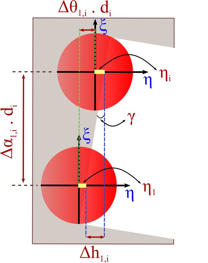
Remote Sens. 2021, 13, 615                                                                                            2 of 23

                                  The resolution capability of laser scanners has been investigated experimentally by
                             several authors. Reference [17] carried out a general analysis of various indicators of laser
                             scanner accuracy based on data acquired experimentally with commercial scanners on
                             specifically designed targets, including observations of the influence of mixed pixels on
                             effective resolution and edge effects. References [16,18] used optical transfer function
                             analysis to define a unified metric that accounts for the joint impact of scanning resolution
                             and beam size, demonstrating that the effective RC is only reliably defined by the selected
                             scanning resolution when the latter is much larger than the laser footprint. Reference [19]
                             evaluated the interplay between scanning resolution and beam divergence empirically to
                             derive practical insights for the appropriate choice of the scanning resolution and scanning
                             configuration in view of the required level of detail of the resulting point cloud. Following
                             the approach of [17] and using ad-hoc targets [15,20,21] focused on extensive experimental
                             investigations of the RC of specific instruments, providing practical recommendations
                             about the suitability of certain scanners and settings for given requirements in terms of
                             level of geometric details represented by the point cloud.
                                  Herein, we complement these investigations by providing an analytical expression
                             for predicting the angular resolution capability as a function of beam properties and
                             additionally relevant parameters, namely distance, distance noise, surface reflectivities and
                             modulation wavelength. We focus on phase-based LiDAR (light detection and ranging)
                             which uses modulated continuous waves. This technology is the backbone of some of the
                             most precise commercially available terrestrial laser scanners for short to medium ranges,
                             requires no algorithmic design choices like signal detection thresholds or full wave-form
                             analysis potentially affecting the RC, and cannot be tuned to separate multiple reflections
                             within the same beam. We derive the analytical expression from a numerical model of
                             the mixed pixel effect and simplify it by focusing on the most influential parameters. Our
                             main contribution with respect to previous investigations on RC lies in providing a simple
                             expression which bounds the RC that can be expected from a certain scanner and scanning
                             scenario, and which requires only parameters that can in most cases be obtained directly
                             from the manufacturer’s specifications or simply approximated.
                                  Our models of mixed pixels and RC are based on the assumption of a Gaussian
                             beam [22–24]. If the beam waist diameter and the beam divergence are given in the
                             instrument’s data sheet, the resolution capability can be predicted with practically useful
                             accuracy using only the data sheet and the equations given herein. However, currently the
                             data sheets rarely contain these values or the necessary quantities allowing to calculate
                             them unambiguously. As an additional contribution, we therefore introduce a simple
                             procedure to derive sufficient approximations of the beam parameters experimentally, from
                             scans across an edge between a planar foreground and a planar background. The MATLAB
                             functions for calculating the beam parameters from the scans are provided on GitHub:
                             https://github.com/ChaudhrySukant/BeamProfiling (accessed on 2 February 2021).
                                  The paper is structured as follows—Section 2 briefly presents the mathematical model
                             of phase-based LiDAR measurements. In Section 3 we derive an analytical model for the
                             mixed pixel effect at a single edge between parallel planar foreground and background
                             of possibly different reflectivity. We also establish the relation to the resolution capability.
                             In Section 4 we show the experimental setup for a mixed pixel analysis and for determining
                             the relevant beam parameters. We briefly refer to the numerical simulation framework
                             used for validation of the simplified analytical expressions. Section 5 shows experimental
                             results comparing predicted and observed mixed pixel effects. In Section 6 we compare
                             the RC for three scanners and different settings obtained from our analytical model to
                             the results reported by [15,21] who used a specially designed target for an experimental
                             investigation. The conclusions are given in Section 7.

                             2. Phase-Based LiDAR
                                 Phase-based LiDAR systems estimate the distance to the illuminated targets from the
                             accumulated phase of radio-frequency tones modulated onto a continuous-wave (CW)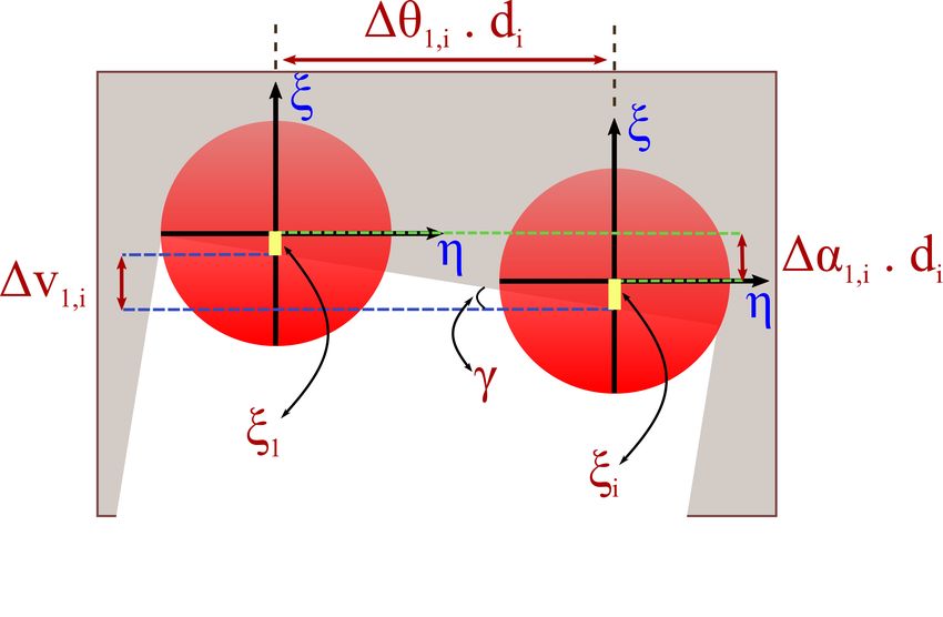
Remote Sens. 2021, 13, 615                                                                                          3 of 23

                             laser [25]. The phase is an indirect observation of the propagation time of the optical
                             probing signal. Assuming that the measurement refers to a single point at the euclidean
                             distance d from the mechanical zero of the instrument, the phase observation φ̂λm at a
                             certain modulation wavelength λm can be written as

                                                                       4π
                                                           φ̂m = mod      (d − k0 ) + ε ,                         (1)
                                                                       λm

                             where ε represents the measurement error and k0 the systematic distance offset between
                             the internal phase reference of the instrument and its mechanical zero, compensated
                             by calibration. The estimated distance dˆm to the target can be derived from this phase
                             observation as
                                                                     λm        λm
                                                               dˆm =    φ̂m +     Nm + k0 ,                            (2)
                                                                     4π         2
                             where Nm is the (unknown) number of full cycles covered by the modulation wave-
                             length λm .
                                  For real LiDAR measurements the beam is actually reflected by a finite patch of sur-
                             face rather than at a single point. The observed phase therefore represents the weighted
                             contributions of the signals reflected across the beam footprint F on the surface. These con-
                             tributions experience different delays and attenuation depending on the surface geometry
                             and reflectance properties across F . Considering the phasor sum of all contributions, the
                             observed phase can be expressed as

                                                                                    Îm
                                                                φ̂m = arctan              ,                            (3)
                                                                                   Q̂m

                             where the quadra- and in-phase components Q̂m and Îm are actually measured by the
                             instrument [26,27]. They result from mixing the received signal with an attenuated copy of
                             the simultaneously emitted signal and of a delayed version of it, as is for example, also
                             known from GPS carrier phase tracking, see for example, [28]. These components are
                             functions of the distances d(·) and reflected optical powers p(·) within F , such that
                                                       ZZ
                                                                             4π
                                                 Îm =      p(α, θ ) · sin       [d(α, θ ) − k0 ] dαdθ + ε I        (4a)
                                                          F                  λm
                                                       ZZ
                                                                             4π
                                                Q̂m =       p(α, θ ) · cos       [d(α, θ ) − k0 ] dαdθ + ε Q ,      (4b)
                                                          F                  λ m

                             where ε I and ε Q are the measurement errors, and the footprint is expressed as the subset of
                             angles α and θ (in orthogonal directions) from the beam axis for which the irradiance on
                             the surface is relevant.
                                  We will further specify and simplify this general model for the phase observations in
                             the next section by considering only a limited number of reflected contributions in order to
                             derive a model of the mixed-pixels bias. A more detailed explanation of the phase-based
                             LiDAR measurement process can be found in [27].
                                  As is apparent from Equations (1) and (2), the number of full cycles Nm is unknown,
                             making phase-based distance measurements inherently ambiguous for ranges larger than
                             λm /2. This is practically solved by combining two or more modulation wavelengths and
                             thus extending the overall unambiguous range across the complete measurement range
                             of the instrument. We base our analysis herein on an incremental ambiguity resolution
                             approach, that represents the simplest solution for multi-wavelength distance measurement.
                             This approach relies on using a longer wavelength to solve the cycle ambiguity of the
                             (immediately next) shorter wavelength, see for example, [25]. The actually used modulation
                             wavelengths of modern laser scanners are usually not communicated by the manufacturers,
                             but the shortest ones may be expected to be on the order of about 1 m, as established
                             for electronic distance meters, [25] and also indicated by the values reported about an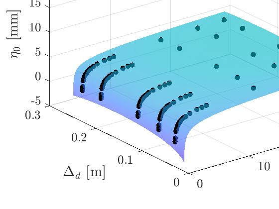
Remote Sens. 2021, 13, 615                                                                                           4 of 23

                             older Faro scanner in [12] (2.4 m). It requires the uncertainty of the measurement at the
                             longer wavelength to be less than the shorter wavelength. Once unambiguous, the final
                             measurement is uniquely defined by the shortest wavelength, which provides the highest
                             resolution and precision.
                                  Given a phase observation φ̂l at a modulation wavelength λl > 2dmax where dmax
                             is the maximum possible range of the instrument, and ignoring k0 for simplicity, an
                             unambiguous distance estimate can be directly obtained from

                                                                          λ
                                                                     dˆl = l φ̂l .                                      (5)
                                                                          4π
                                 This measurement is then used to select the number Nm of full cycles of the shorter
                             wavelength λm that provides the highest agreement, that is,

                                                                          λm       λm
                                                   Nm = arg min dˆl −        φ̂m +     N    ,                    (6)
                                                            N             4π        2

                             with φ̂m being the observed phase at λm , and λm larger than the uncertainty of dˆl . This
                             enables an absolute distance estimation dˆm based on the smaller wavelength λm , therefore
                             more precise than dˆl under the same measurement conditions.
                                  This process can be carried out sequentially with more than two wavelengths. The
                             choice of wavelengths and ambiguity resolution approach by the manufacturer is a trade-
                             off between maximum range, desired distance resolution, and implementation complexity.
                             However, the mixed-pixel behaviour for targets separated by a few cm to dm only—and
                             thus the resolution capability as studied herein—is dominated by the distance bias at the
                             smallest modulation wavelength. In this case, the ambiguity resolution algorithm has
                             virtually no influence on the RC and we therefore use the above simple algorithm without
                             further investigation herein.

                             3. Mixed Pixel and Resolution Capability Models
                                  Based on a simple but representative situation, we develop an analytical model of the
                             mixed-pixel bias in this section. We then use this model to derive an approximation of the
                             RC which accounts for the impact of both scanning resolution and footprint spatial averag-
                             ing. The validation of the mixed-pixel model by direct comparison with our laser scanning
                             numerical simulation framework [27] is presented in Section 5.1. The RC approximation is
                             validated in Section 6 by comparison to previously published experimental results.

                             3.1. Mixed Pixel Bias
                                  We assume an elliptical Gaussian measurement beam [24,29] illuminating simultane-
                             ously two perfectly planar and homogeneous targets parallel to each other and oriented
                             normally to the beam axis. The transition between both targets is assumed to be a perfectly
                             straight edge within the footprint dimensions. Figure 1 shows front (a) and top (b) view
                             diagrams of this situation depicting both targets. The targets are defined by their respective
                             spatially invariant reflectances R1 and R2 , and are placed at distances d1 and d2 = d1 + ∆d
                             from the instrument, respectively, where we assume that ∆d
Version February 2, 2021 submitted to Remote Sens. 5 of 23
Remote Sens. 2021, 13, 615 5 of 23
132 While the figure represents a transition between targets along a vertical edge and the following
133 derivations are therefore specified for the horizontal beam dimension η, the analysis resulting therefrom
analysis resulting therefrom is equally valid for the vertical dimension ξ when the beam
134 is equally valid for the vertical dimension ξ when the beam transits across a horizontal edge.
transits across a horizontal edge.
Background
Background
Background Foreground
Foreground
Foreground Background
Background
Background Foreground
Foreground
Foreground
Background
Background
Background
Foreground
Foreground
Foreground
Beam axis
Beam axis
Beam axis
(a)
(a)
(a) (b)
(b)
(b) (c)(c)
(c)
(a) (b) (c)
Figure 1. Modeled mixed pixel scenario with Gaussian footprint of 1/e2 horizontal radius 2σb covering a vertical transition
Figure 1. Modeled
planarmixed pixel scenario with Gaussian
targetsfootprint of 1/eR2 horizontal radius 2σ covering
between orthogonal foreground and background of reflectance 1 and R2 at distancesb d1 and d1 + ∆d ,
a vertical transition between orthogonal planar foreground and
respectively. (a) Front view, (b) top view, and (c) beam irradiance profile. background targets of reflectance R1
and R2 at distances d1 and d1 + ∆d , respectively.
For distances much larger than the footprint diameter, as is the case for terrestrial
For distances much larger
laser than the
scanning (with footprint diameter,ofasseveral
typical distances is the case
m or for terrestrial
more, laserbeam
and typical scanning
diameters
(with typical distances of several m or more, and typical beam diameters at the mm- to cm-level) except the
at the mm- to cm-level) except at close range and with extremely flat beam incidence,
at close range and with distance variations
extremely flat beamwithin the footprint
incidence, portion on
the distance each planar
variations targetthe
within can be neglected
footprint
and the measurement process can be approximated as a
portion on each planar target can be neglected and the measurement process can be approximatedweighted average of twoassingle-
point measurements where each reflecting surface is represented by a single distance.
a weighted average of two single-point measurements where each reflecting surface is represented
Considering the quasi-normal incidence on both targets, the distances can be approximated
by a single distance. as Considering
d1 and d1 + ∆the quasi-normal incidence on both targets, the distances can
d , respectively. The weights W1 and W2 , on the other hand, are proportional
be approximated as d1toand d1 + ∆signal
the optical d , respectively. The from
power received weights W1 andand
foreground , on the other
W2background, hand, arewhere
respectively,
proportional to the optical
we may signal
assume power
equalreceived
attenuationfromdueforeground andatmosphere
to distance and background, for respectively,
both. The weights
where we may assumecan thusattenuation
equal be calculated as the
due integral of
to distance andtheatmosphere
irradiance over the respective
for both. The weightsportion
canof the
footprint, scaled with the surface reflectance. Since we assumed that
thus be calculated as the integral of the irradiance over the respective portion of the footprint, scaledthe separation between
the targets is much smaller than the distance to the front target, the beam divergence
with the surface reflectance. Since we assumed that the separation between the targets is much smaller
between the targets can be neglected, and the integration can be carried out over the
than the distance to the front target,
irradiance at thethe beam divergence
foreground between
distance, that is, the targets can be neglected, and
the integration can be carried out over the irradiance at the foreground distance, i.e.
Z +∞
Z +∞ W1 = R1 E(η, d1 )dη (7a)
ηe
W1 = R1 E (η, d1 ) Zdηηe
(7a)
ηe
Z ηe W2 = R2 E(η, d1 )dη, (7b)
−∞
W2 = R2 E (η, d1 ) dη (7b)
−∞edge on the η-axis.
where ηe is the location of the
As discussed in Section 2, the estimated distance dˆm is derived from the phase ob-
135 where ηe is the location of the edge on the η-axis.
servation φ̂m at the shortest modulation wavelength λm , and the ambiguity is resolved
As discussed in Section 2, the estimated distance dˆm is
using larger wavelengths. Considering
derived from the phase observation φ̂
the derivation of the phase observation frommthe I-
at the shortest modulation wavelength λmand
and Q-components, , and therespective
their ambiguity is resolved
definition using to
according larger wavelengths.
Equation (4), the phase
Considering the derivation of the phase
observation observation
for the from the I-
shortest wavelength is and Q-components, and their respective
definition according to eq. (4), the phase observation for the shortest wavelength is
d1 4π (d1 +∆d )4π
φ̂ = arctan W1 sin λm + W2 sin λm . (8)
m 1 + ∆d )4π
d(1d4π
W1 sin dλ1 4π + W
W 2
1
sin
cos λ+ W 2 cos
(d1 +∆d )4π
φ̂m = arctan m λ m m λ m . (8)
(d1 +∆d )4π
W1 cos dλ1 4π + W2 cos
The distance dˆm is then calculated from this phase according to Equation (2), where
m λm
the number Nm of full cycles is resolved from an additional measurement using a longer
136 The distance dˆm is then calculated
wavelength, asfrom this in
discussed phase according
Section 2. to eq. (2), where the number Nm of
137 full cycles is resolved from an additional measurement using a longer wavelength, as discussed in
138 Section 2.
Remote Sens. 2021, 13, 615                                                                                            6 of 23

                                  The impact of mixed pixels on phase-based LiDAR is twofold and depends in particu-
                             lar on the range of distances involved. If the separation ∆d between the targets is smaller
                             than λm /4, the mixed pixel situation has no impact on the ambiguity resolution and only
                             the phase of the smallest wavelength is affected. This case is modeled by Equation (8). The
                             error introduced in this case results in a distance estimate somewhere between the true
                             distances of both targets. Assuming a footprint that slides gradually across the edge, the
                             distance changes smoothly between both true values and the distance error depends on
                             the relative weights. When larger relative distances are involved, the ambiguity resolution
                             algorithm yields different values for Nm with the beam center in the vicinity of the edge,
                             depending on the actual distances, on the measurement noise and on the relative weights.
                             This introduces an apparent quantization and produces estimated distances only near
                             integer multiples of λm /2 in the region affected by mixed-pixels. When visualizing a point
                             cloud this phenomenon appears as a set of equidistant, noisy replicas of the foreground
                             contour towards the background. However, also in this case the resolution capability is
                             affected by spatial averaging within the footprint and is fundamentally limited by the
                             mixed pixel biases. This contribution to RC is therefore the focus of the model derived next.
                                  Considering the foreground distance to be the true distance, the mixed-pixel bias
                             for a specific edge between foreground and background (with specific reflectances and
                             at specific distances) depends on the distance of the beam center from the edge. From a
                             practical perspective, there will be no (significant) mixed-pixel bias if the beam center is far
                             enough from the edge. We now aim at deriving an equation which predicts how close to
                             the edge—or possibly even beyond it—the beam center can be such that the mixed-pixel
                             bias is negligible. This will allow us to draw conclusions about the location and width of
                             the regions around the target edges that are prone to significant errors. We define these
                             errors as significant when they are larger than a threshold τ which we link to the expected
                             noise level σn of the LiDAR sensor as τ = 0.5σn .
                                  Taking the front target as a reference and thus assuming that d1 is the true distance,
                             we determine the critical (minimum) ratio QW    min between the weights W and W for which
                                                                                                         2      1
                             the distance error exceeds the threshold:

                                                                  min     W2
                                                                 QW   =                     .                            (9)
                                                                          W1   dˆm =d1 +τ

                                  It can be calculated from (2) and (8) as

                                                         tan (d1 + τ ) λ4πm cos d1 λ4πm − sin d1 λ4πm
                                           min                                                                .
                                         QW    =                                                                   (10)
                                                 sin (d1 + ∆d ) λ4πm − tan (d1 + τ ) λ4πm cos (d1 + ∆d ) λ4πm

                                  The weights can be related to the beam properties by calculating the normalized
                             power P1 in the foreground target through integrating the Gaussian irradiance profile,
                             defined by its shape parameter σb at d1 , along the dimension η perpendicular to the edge.
                             This yields
                                                                  1                ηe
                                                           P1 =        1 + erf     √     ,                         (11)
                                                                  2              σb 2
                             where erf(·) is the Gauss error function as resulting from integrating the probability
                             density function of a normal distribution. Considering that the normalized power in
                             the background is (1 − P1 ), we obtain

                                                                   W2  R (1 − P1 )
                                                                      = 2          .                                    (12)
                                                                   W1     R1 P1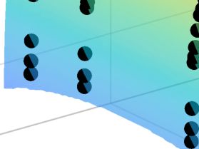
Remote Sens. 2021, 13, 615                                                                                           7 of 23

                                  Plugging this and Equation (11) into (9), rearranging to express the position ηe of the
                             edge within the footprint, and denoting this particular position (where the ratio of W2 and
                             W1 is exactly the critical ratio) η0 , we obtain:
                                                                                          −1   !
                                                             √                 min  R1
                                                     η0 = σb 2 · inverf QW ·           +1      −1 ,                  (13)
                                                                                   2R2

                             with inverf(·) being the inverse Gauss error function. Since there exists no closed form rep-
                             resentation of this function, the above expression needs to be evaluated using a numerical
                             approximation of inverf.
                                  From the perspective of the scanning process, this derivation provides a solution for
                             calculating the critical distances η0 around the edge of certain targets within which the
                             impact of mixed pixels may become visible over the noise background. Results from the
                             evaluation of this expression and a validation are presented and discussed in Section 5.1.

                             3.2. Resolution Capability
                                   The mixed pixel model derived above can easily be extended to compute the width
                             of the transition region between two targets where measurements cannot be resolved
                             independently for one of the targets, thus indicating the resolution capability as limited by
                             footprint spatial averaging. For this purpose, we need to complement the above η0 by the
                             critical value η00 that conceptually corresponds to η0 but denotes the position of the edge
                             within the footprint where the mixed pixel bias first exceeds the threshold when moving the
                             beam towards the edge from the background side and considering the background distance
                             as the true distance. This edge position is obtained by replacing QW min in Equation (13) with

                                                               max     W2
                                                              QW   =                         .                        (14)
                                                                       W1   dˆm =d1 +∆d −τ

                                   The resolution capability RC can then be calculated as the width of the region between
                             the limits η0 and η00 where measurements do not correspond reliably to any of the targets as

                                                                    RC = η0 − η00 .                                   (15)

                                  To analyze the impact of the separation and reflectances of foreground and background
                             targets on RC , the derived resolution capability model has been computed for certain
                             arbitrary but realistic instrument parameters. The resulting values for ∆d between 0 and
                             λm /4, and reflectance ratios R2 /R1 between 0.1 and 10 are depicted in Figure 2, where the
                             absolute maximum (largest value of RC ) is indicated with a black dot. Equivalently to the
                             mixed pixel biases, as modeled in Section 3.1, the resolution capability shows a periodicity
                             of λm /4 with the target separation ∆d . For such target separations the contributions of
                             foreground and background to the overall phase at λm are almost in phase or in phase
                             opposition and thus the mixed pixel situation primarily affects the total signal power while
                             the distance measurement changes from foreground to background nearly suddenly as the
                             beam sweeps across the edge. However, this situation is not practically relevant because of
                             the impact of measurement noise. Furthermore, we restrict the RC analysis herein to small
                             target separations, that is, ∆d < λm /4, as mentioned above.
                                  As can be seen in Figure 2a, the (practically relevant) maximum value of RC occurs at
                             λm /8. Figure 2b shows RC as a function of the reflectance ratio for this particular target
                             separation. This shows more clearly than Figure 2a that the resolution capability depends
                             slightly on the ratio of the reflectances and is largest when R1 = R2 .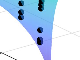
Version
Remote Sens. 2021,February
13, 615 2, 2021 submitted to Remote Sens. 8 of8 of
2323
20
18
16
14
12
10
10-2 10-1 100 101 102
(a) (b)
Figure 2. Resolution capability computed for a beam diameter (1/e2 of 12.8 mm, range noise σn = 1 mm and fine
2. Resolution 2 of 12.8 mm, range noise σ = 1 mm
Figure
modulation wavelength λm =capability computed
1 m: (a) as forofatarget
a function beam separation
diameter (1/e
∆d and reflectance ratio R2 /R1 nand, (b) as a
and fine modulation wavelength
function of reflectance ratio for fixed ∆d = λm /8.
λ m = 1 m: (a) as a function of target separation ∆d and reflectance
ratio R2 /R1 and, (b) as a function of reflectance ratio for fixed ∆d = λm /8.
Aiming at providing a simple expression that enables computing the resolution capa-
bility with little information on the scanner and scene properties, we have simplified the
where inverf (·) is theabove
inverse Gauss
model error
by only function,
focusing on the worst case described above, that is, a target separation
∆d = λm /8 and equal reflectances (R1= R2 ) of the foreground and background planes.
This results in min 4π
QW = tan τ (17a)
" λm# !
√
min − 1 max −1
QW π+ 1 4π QW
RC = σb 2Q max
inverf = tan − τ − 1 − inverf +1 − 1 , (17b) (16)
W 2 2 λ 2
m
and the beam shape parameter
where inverf atisthe
σb(·) themeasurement
inverse Gauss distance d1 can be calculated from the nominal
error function,
or measured beam parameters following the Gaussian beam model [21–23] as
min 4π
s QW = tan τ (17a)
λ
m
w0 ) π2 4π
Θ (d1 − f 0
σb ≈ 1+ Q max
= tan , τ
− (18)
(17b)
2 W w 0 2 λm
186 with Θ being the beam and the beam shape
divergence parameter
half-angle, σb at1/e
w0 the the2 measurement distanceand
beam waist radius, d1 can
f 0 be
thecalculated
beam waistfrom
the nominal or measured beam parameters following the Gaussian beam model [22–24] as
187 distance from the mechanical zero of the instrument.
s
Laser scanners typically realize the vertical beam deflection by means of a fast continuously
w0 Θ ( d1 − f 0 ) 2
rotating mirror. Additionally, phase-based LiDARb sensorsσ ≈ 1internally
+ ,
accumulate the I and Q samples (18)
2 w0
as of eq. (4) over some time (integration time, herein) to collect enough signal power for a potentially
Θ being
with and 2 beam waist radius, and f the
high signal-to-noise ratio thusthe beam
high divergence half-angle,
measurement precision.w0Ifthethe1/e
integration time during each 0
beam waist distance from the mechanical zero of the instrument.
measurement is not much smaller than the time between subsequent vertical measurements, the
Laser scanners typically realize the vertical beam deflection by means of a fast contin-
beam displacement during the integration introduces an effective elongation of the beam vertical
uously rotating mirror. Additionally, phase-based LiDAR sensors internally accumulate
dimension. The model thecan
I and beQextended
samples astoofaccount
Equationfor (4)this
overeffect when
some time specifically
(integration time,calculating the
herein) to collect
vertical resolution capability
enough by modifying
signal power for thea nominal
potentiallybeam
highparameters
signal-to-noise to calculate
ratio andathus
specific
highvertical
measure-
beam shape parameter ment . Approximating
σb,vtprecision. σb,vt as the
If the integration timesum of the
during each nominal
measurementbeam is shape parameter
not much smaller
σb (corresponding to than the time
a static between
beam) subsequent
and the apparent vertical
beammeasurements, the beam displacement
elongation resulting during
from the vertical
the integration introduces an effective elongation of the beam
displacement of the beam during the integration time (during which the beam constantly illuminates vertical dimension. The
model can be extended to account for this effect when specifically calculating the vertical
the surface but movesresolution
vertically), we obtain
capability by modifying the nominal beam parameters to calculate a specific
vertical beam shape
s parameter σb,vt . Approximating σb,vt as the sum of the nominal beam
Θ (d1 − f 0 ) to2a static
w0 σb (corresponding
shape parameter 1 beam) and the apparent beam elongation
σb,vt ≈ 1+ + Kint · d1 · ωRS , (19)
2 w0 4
188 where ωRS = RS /d1 is the angular scanning resolution of the instrument as chosen by the user,
189 Kint ∈ (0, 1] represents the ratio between the measurement integration time and the time between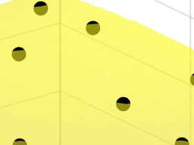
Remote Sens. 2021, 13, 615                                                                                              9 of 23

                             resulting from the vertical displacement of the beam during the integration time (during
                             which the beam constantly illuminates the surface but moves vertically), we obtain
                                                               s
                                                                                            2
                                                          w                 Θ ( d1 − f 0 )         1
                                                 σb,vt   ≈ 0       1+                             + Kint · d1 · ωRS ,    (19)
                                                           2                     w0                4

                             where ωRS = RS /d1 is the angular scanning resolution of the instrument as chosen by
                             the user, Kint ∈ (0, 1] represents the ratio between the measurement integration time and
                             the time between subsequent measurement points (Kint = 1 would indicate integration
                             across the complete transition between subsequent points), and the coefficient 1/4 intro-
                             duces the ratio between the beam shape parameter and the 1/e2 beam diameter. This
                             extension is useful to provide a more realistic estimation of the vertical degradation of
                             the resolution capability depending on the chosen scanning resolution and quality setting
                             (longer integration time for higher quality). However, it requires Kint to be estimated
                             beforehand; the actual integration times for different scanner settings are usually not given
                             in the specifications or manuals.
                                  The simplified expressions in (16) to (19) provide a worst case estimation of the
                             resolution capability that represents a useful indicator of the overall expected performance
                             while only requiring knowledge of the distance to the targets of interest and the basic beam
                             properties (divergence, waist radius and waist position), noise level and fine modulation
                             wavelength of the instrument. Unlike beam properties and range noise, typically provided
                             in the instruments’ specifications, the modulation wavelengths implemented in laser
                             scanners are not usually disclosed by the manufacturers. Nevertheless, since range noise
                             levels are in any case much smaller than the fine modulation wavelength, uncertainties
                             in the value used for the above equations do not have a large impact on the computed
                             resolution capability. For example, under realistic instrument parameters a deviation of
                             50% on the applied wavelength introduces deviations below 7% on the computed value of
                             RC . In case no information at all is available regarding modulation wavelength, a value of
                             1 m is a reasonable choice considering current bandwidth limits in the hundreds of MHz
                             range for commercially available modulators.
                                  Aiming at providing an integral indicator of the expected resolution capability, the
                             derived model for mixed-pixel limited resolution capability RC should be extended to
                             account also for the influence of scanning resolution. Although the interplay between
                             mixed pixels and scanning resolution may require a more specific investigation and is
                             beyond the scope of this paper, we define a simple approximation for the total resolution
                             capability RC 0 by adding the angular scanning resolution ω
                                                                                            RS such that

                                                                    RC0 = RC + d1 · ωRS .                                (20)

                                  As opposed to Equation (19) which introduces an effective beam elongation only in
                             the vertical direction (the integration time has virtually no influence on the horizontal beam
                             shape), Equation (20) holds for both, horizontal and vertical RC. It takes into account that
                             an object can only be resolved if it is wider than both the mixed-pixel zone and the distance
                             between neighboring points in the point cloud.

                             4. Practical Approach for Mixed Pixel Analysis
                                  In this section, we present the experimental measurement setup and the simulation
                             framework used for the quantitative analysis of mixed pixel effects and for the validation
                             of the equations derived above. Ideally, the experiments would yield measurements for
                             different positions of the footprint center with respect to an edge and allow the footprint
                             to be shifted in small increments from the beam being fully on the background to being
                             fully on the foreground. This can be achieved easily with the numerical simulations
                             (see Section 4.2). However, it is virtually impossible to achieve this movement of the
                             footprint across an edge experimentally using a commercial terrestrial laser scanner which
Remote Sens. 2021, 13, 615 10 of 23
yields measurements at fixed, user-selected angular increments ωRS . We solve this problem
in Section 4.1 by proposing a special target configuration for the scans.
4.1. Experimental Investigation
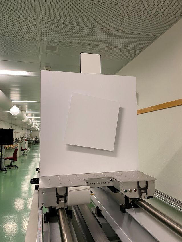
In order to obtain a sufficient number of mixed pixels and a large variety of relative
footprint positions with respect to the edge from a normal scan, we use a square foreground
plane which is slightly rotated such that neighboring points along vertical or horizontal
profiles in the point cloud are associated with different footprint fractions on the foreground
and background, see Figure 3 and explanations below. For practical reasons we have
mounted the targets on a trolley which can be moved along a linear bench and enabled
easily scanning the targets from different distances using a laser scanner set up at one
end of the bench. The relative distance between the foreground and background planes
can be changed manually between 3 and 23 cm. This range covers approximately the
region where predicting the mixed pixel effects does not require assumptions regarding
the ambiguity resolution algorithm (see Section 2). Additionally, we mounted a diffuse
reflectance standard above the background target, see Figure 3, to enable estimation of
the foreground and background reflectances from the scanner’s intensity data. Knowing
the reflectances is not necessary for predicting the RC using our analytical model (see
Equations (16) to (19)), but it allowed simulating exactly the real measurement situation
later on. For all our own experiments reported herein, we used a Z&F Imager 5016 scanner,
foreground and background plates with the same reflectance (73%), and a setup where the
Version February 2,scanner is upright
2021 submitted and
to Remote Sens.approximately at the same height as the target center such
10 of 23 that the
beam hits the targets almost orthogonally across the entire target surface.
10°
10°
30 cm
60 cm
30 cm
60 cm
(a) (b)
Figure 3. Target configuration of the experimental set-up. (a) Motorized trolley equipped with
Figure 3. Target configuration of the experimental set-up. a) Motorized trolley equipped with
foreground plate, background plate and Spectralon reference target. (b) Dimensions and placing of
foreground plate, background plate and Spectralon reference target. b) Dimensions and placing
the target components.
of the target components.
Analyzing the mixed pixel effects requires a quantification of the relative portion of
230 along a linear bench and enabled
the footprint easily
on each scanning
of the theThis
targets. targets from different
is possible distancesthe
by calculating using a laser ∆η and
differences
231 scanner set up at one end of the bench. The relative distance between the foreground and background
∆ξ of the foreground-background edge position within the footprint (see Section 3.1 for the
232 planes can be changed manually
definition of η andbetween
ξ) from3 the
anddifferences
23 cm. This∆θrange
andcovers
∆α of approximately the region
the polar coordinates of points in
233 where predicting the mixed pixel effects does not require assumptions regarding the ambiguity
the point cloud. The relevant parameters of this transformation for the quasi-vertical and
234 resolution algorithm (see Section 2). Additionally,
the quasi-horizontal we mounted
edge are depicted a diffuse
in Figure 4. reflectance standard above the
235 background target, see Figure 3, to enable estimation of the foreground and background reflectances
236 from the scanner’s intensity data. Knowing the reflectances is not necessary for predicting the RC using
237 our analytical model (see eqs. (16) to (19)), but it allowed simulating exactly the real measurement
238 situation later on. For all our own experiments reported herein, we used a Z&F Imager 5016 scanner,
239 foreground and background plates with the same reflectance (73%), and a setup where the scanner is
240 upright and approximately at the same height as the target center such that the beam hits the targets
241 almost orthogonally across the entire target surface.
242 Analyzing the mixed pixel effects requires a quantification of the relative portion of the
243 footprint on each of the targets. This is possible by calculating the differences ∆η and ∆ξ of the
244 foreground-background edge position within the footprint (see Section 3.1 for the definition of η and
245 ξ) from the differences ∆θ and ∆α of the polar coordinates of points in the point cloud. The relevantRemote Sens. 2021, 13, 615 11 of 23
Version February 2, 2021 submitted to Remote Sens. 11 of 23
(a) Quasi-vertical edge (b) Quasi-horizontal edge
Figure 4. Parameters involved in the transformation between scanner coordinate system and footprint
Parameterssystem.
Figure 4.coordinate involved in the transformation between scanner coordinate system and footprint
coordinate system.
The vertical movement of the footprint is depicted in Figure 4a which shows two
250
points near the edge,
assumed to be approximately onefor
equal of both
which we arbitrarily
points, i.e. d1 ≈picked fromγ,
di . Except theallpoint cloud can
quantities as reference
be
251
point for this analysis and denoted with the index
extracted directly from the measured coordinates output by the scanner.1, the other one arbitrarily assumed to
be the ith picked
The transformation for thepoint. η1 and
footprint ηi are the along
displacement positions of the(see
the ξ-axis edge relative
Figure 4b) to the respective
is achieved
footprint center along the η-axis. The relative change ∆η of the footprint center
equivalently, where we assume the same tilt angle γ as above, now as the1,iangle between the scanner’s position
with
horizontal axis andrespect to the edge when moving from point 1 to point i is
the edge:
∆ξ 1,i = ∆v1,i − ∆α1,i · di , (23)
∆η1,i = ∆h1,i + ∆θ1,i · di , (21)
with
where ∆v1,i = tan(γ) · ∆θ1,i · di . (24)
∆h1,i = tan(γ) · ∆α1,i · di (22)
252 These transformations are applied to the sections of the point clouds used for the mixed pixel
253
is the shift
analysis obtained from resulting from the measurements.
the experimental tilt angle γ between the edge andmeasurements
The transformed the scanner’s vertical
enable axis,
254
∆θ 1,i and ∆α 1,i are the differences of the horizontal and vertical angles of the two points,
representing the estimated distances uniquely as a function of the relative displacement of the footprint
255
and d is the 3d distance assumed to be approximately equal for both points,
center with respecti to the edge independently of the actual scanning process. Although still lackingthat is, d1 ≈ di .
256
Except γ, all quantities can be extracted directly from the measured coordinates
information on the actual position of the edge—which is not known beforehand but will be derived output by
257
the scanner.
from the measured points as part of the further analysis—the resulting data allows analyzing the
The transformation for the footprint displacement along the ξ-axis (see Figure 4b) is
258 mixed pixel effect as the footprint slides across the edge between foreground and background, see
achieved equivalently, where we assume the same tilt angle γ as above, now as the angle
259 Section 5.1.
between the scanner’s horizontal axis and the edge:
260 4.2. Numerical simulation
∆ξ 1,i = ∆v1,i − ∆α1,i · di , (23)
261 The numerical simulation framework, presented in [27], refers to phase-based LiDAR
262 measurements with(Section 2). The simulations are extended to a 3D scanning process by deflecting
263 the measurement beam at incremental angular ∆v 1,i = tanThe
directions. ∆θ1,i · di . use a ray tracing approach (24)
(γ) ·simulations
264 to account for the energy distribution within the discretized laser footprint, surface geometry, and
These transformations are applied to the sections of the point clouds used for the
265 reflectivity of the surface material. The surfaces are geometrically represented as triangular irregular
mixed pixel analysis obtained from the experimental measurements. The transformed
266 networks (TIN). The reflectivity properties are associated with the individual triangles via a Lambertian
measurements enable representing the estimated distances uniquely as a function of the
267 scattering model [32,33].
relative displacement of the footprint center with respect to the edge independently of the
268 The simulation framework
actual scanning operates
process. on a Gaussian
Although irradiance
still lacking beam profile
information [22,23]
on the assumption,
actual position of the
269 and allows to configure beam divergence, beam width and optical wavelength,
edge—which is not known beforehand but will be derived from the measured as well as the set of
points as
270 modulation wavelengths used for the phase estimation. For the present paper, we use the framework
part of the further analysis—the resulting data allows analyzing the mixed pixel effect as
271 to simulate measurements like the
the footprint slides onesthe
across described in sec. foreground
edge between 4 but with aand larger number ofsee
background, different
Section 5.1.
272 configurations than in the real experiments. The beam parameters are taken from the specifications
273 of the scanner4.2.used the experimental investigation. The beam divergence Θ is 0.3 mrad
duringSimulation
Numerical
274 (half-angle), which The numerical to
corresponds a beam waist
simulation radius ofpresented
framework, about 1.6 in
mm. The
[27], optical
refers wavelength of
to phase-based LiDAR
measurements (Section 2). The simulations are extended to a 3D scanning process by
deflecting the measurement beam at incremental angular directions. The simulations
use a ray tracing approach to account for the energy distribution within the discretizedRemote Sens. 2021, 13, 615 12 of 23
laser footprint, surface geometry, and reflectivity of the surface material. The surfaces are
geometrically represented as triangular irregular networks (TIN). The reflectivity properties
are associated with the individual triangles via a Lambertian scattering model [32,33].
The simulation framework operates on a Gaussian irradiance beam profile [23,24]
assumption, and allows to configure beam divergence, beam width and optical wavelength,
as well as the set of modulation wavelengths used for the phase estimation. For the present
paper, we use the framework to simulate measurements like the ones described in Section 4
but with a larger number of different configurations than in the real experiments. The beam
parameters are taken from the specifications of the scanner used during the experimental
investigation. The beam divergence Θ is 0.3 mrad (half-angle), which corresponds to a
beam waist radius of about 1.6 mm. The optical wavelength of the laser is 1500 nm, reported
in [21,34]. There is no information about the implemented modulation wavelengths in
the specifications. Judging from replicas produced in mixed pixel experiments with large
separation between foreground and background, we assume that the shortest modulation
wavelength λm is around 1.26 m and use this value herein. A longer modulation wavelength
is only needed for ambiguity resolution. Since the impact of the latter is not investigated
herein and we restrict to an analysis with short foreground-background separation where
the ambiguity resolution does not affect the mixed pixel bias, the choice of the longer
wavelength(s) is not critical. We arbitrarily chose 100 × λm , that is, 126 m, as the single
longer modulation wavelength for the simulations.
5. Experimental Results
This section contains the mixed pixels analysis using the numerical simulation frame-
work and the analytical model, in Section 5.1. Furthermore, in Section 5.2, it shows the
experimental results of the beam parameter estimation of the Z&F Imager 5016 laser
scanner using real measurements according to the procedure proposed in Section 4.1.
5.1. Mixed Pixels
We now study the mixed pixel effect numerically for a set-up equivalent to the one
defined in Section 3. In particular, we use the numerical simulation framework with the
beam parameters specified in Section 4.2 to predict the distances expected when measuring
vertical profiles with negligibly small angular increments across a horizontal edge and we
quantify how close to the edge the beam center can get at either side before the distance
bias becomes significant. At this stage we assume a circular Gaussian beam. Therefore,
the analysis of a horizontal measurement profile across a vertical edge would yield the
same results.
Figure 5 shows instructive examples of the results. The plots depict the estimated
distance as a function of the footprint center position along the profile for certain combina-
tions of parameters. The values significantly affected by mixed pixel biases are shown in
red. They have been identified as those deviating from the geometrical distance along the
beam center by more than τ = 1.25 mm. This threshold has been chosen for demonstration
purposes only. Following the criteria given in Section 3, the threshold should be chosen
smaller than the expected standard deviation of the distances in a real-world application.Remote Sens. 2021, 13, 615
Version February 2, 2021 submitted to Remote Sens. 13 of13
23of 23
R = 4% R = 90%
bg bg
mixed pixels mixed pixels
Rfg = 90% Rfg = 4%
(a) (b)
R = 4% Rbg = 4%
bg
mixed pixels mixed pixels
Rfg = 90% Rfg = 90%
(c) (d)
Figure 5. The transition width of the measurements (blue points) effected by the mixed pixels (red points) computed using
5. The transition
Figure simulation
the numeric frameworkwidth of the
(Section measurements
4.2) (blue points)
for different combinations of effected
foreground byand
the background
mixed pixels (red
reflectances
points)
[(a,c,d): Rfg =computed
90%, Rbg = using the
4%; (b): numeric
Rfg = 4%, Rbgsimulation framework
= 90%], different (Section
foreground 4.2) for[(a,b):
distances different combinations
d1 = 15 m; (c,d): d1 =of
45 m],
foreground and background reflectances
and different relative distances [(a–c): ∆ d = 6.5 cm; (Rfg and
(d): ∆ d = Rbg ), different foreground distances, and different
23 cm].
relative distances.
Figure 5a shows a scenario with a bright foreground at 15 m and a dark background
6.5 cm farther away. The results were obtained using the beam parameters stated in
318 To see how this transition
Section 4.2. zone is affected
The beam by the
divergence distance,
half-angle we
of 0.3 alsoresults
mrad simulated
in a 1/escenarios with
2 footprint diameter
319 different distances. Figure 5c shows the results of such a calculation for a setup and beam parameters the
of 9.6 mm at this distance. When measurements are taken as the footprint moves across
320
background
exactly as before (see Figure surface and
5a) except the transits
distance beyond
which theisedge
nowof45themforeground target, relevant
to the foreground. Aserrors
a
occur if the beam center is closer than 8 mm to the edge. If instead the footprint approaches
321 consequence of the larger distance, the footprint diameter is also bigger (now approximately 27.2 mm).
the edge from the foreground side significant errors occur only when the beam center is
322 The width of the zone affected by mixed
closer than 0.9 mm pixels is 24.2
to the edge. Somm wide,
in this casei.e.
the scales
region roughly
around the proportionally
edge affected by with
mixed
323 distance and like the footprint
pixels isalthough
about 8.9not mmexactly.
wide (approximately corresponding to the footprint diameter),
324 Figure 5d, corresponding to asymmetric
but it is not scenario likeaboutthetheprevious one but
edge because with
of the an difference
large increasedofdistance
foregroundstepand
325
background reflectances.
between foreground and background (note different scaling of distance axis), finally shows that the
Actually, and in correspondence with the derivations given in Section 3.2, the numeri-
326 impact of a larger relative distance between the two targets is comparably small; the transition zone is
cal simulations showed that the width of the mixed pixel zone is practically independent of
327 only slightly wider thanthe before (26.2 mm),
reflectances, but theand the relative
critical distanceslocation
from theof thatbeyond
edge zone about
which the edgeis does
the bias relevant,
328 not change as compared to 5c. Also these results are in agreement with the theoretical
strongly depend on the ratio of the reflectances. This is corroborated by Figure 5b where findings in the
329 Section 3.2. entire measurement setup is equal to the one of Figure 5a except the reflectances which are
330 Using the numerical interchanged.
simulationThe of width of the affected process,
the measurement zone is equal to the actually
we have previous one (9 mm) but
calculated thethis
331 critical distances η0 to the target edge for a variety of combinations of reflectances (4, 20, 50, 70 andside.
zone now extends from 1.7 mm on the background side to 7.3 mm on the foreground
To see how this transition zone is affected by the distance, we also simulated scenarios
332 90%), distance steps (3, 6.5, 11, 19 and 23 cm), all lying within one quarter of λm ,aand
with different distances. Figure 5c shows the results of such
for both distances
calculation for a setup and
333 (15 and 45 m). The resultsbeamare shown as
parameters blackasdots
exactly in (see
before Figure 6. The
Figure semitransparent
5a) except surfaces
the distance which also45 m
is now
334 shown in this figure were to instead obtained
the foreground. Asfor a dense gridofofthe
a consequence reflectances and distance
larger distance, steps
the footprint using the
diameter is also
335 analytical approximation eq. (13) derived in Section 3. The results agree at the sub-mm level which
336 shows that the analytical approximation can be used to predict the critical distances and the width of
337 the zone affected by mixed pixels.Remote Sens. 2021, 13, 615 14 of 23
bigger (now approximately 27.2 mm). The width of the zone affected by mixed pixels is
24.2 mm wide, that is, scales roughly proportionally with distance and like the footprint
although not exactly.
Figure 5d, corresponding to a scenario like the previous one but with an increased
distance step between foreground and background (note different scaling of distance
axis), finally shows that the impact of a larger relative distance between the two targets is
comparably small; the transition zone is only slightly wider than before (26.2 mm), and
the relative location of that zone about the edge does not change as compared to Figure 5c.
Also these results are in agreement with the theoretical findings in Section 3.2.
Using the numerical simulation of the measurement process, we have actually calcu-
lated the critical distances η0 to the target edge for a variety of combinations of reflectances
(4, 20, 50, 70 and 90%), distance steps (3, 6.5, 11, 19 and 23 cm), all lying within one quarter
of λm , and for both distances (15 and 45 m). The results are shown as black dots in Figure 6.
The semitransparent surfaces also shown in this figure were instead obtained for a dense
grid of reflectances and distance steps using the analytical approximation Equation (13)
Version February 2, 2021 submitted
derivedto Remote Sens.3. The results agree at the sub-mm level which shows that the14
in Section of 23
analytical
approximation can be used to predict the critical distances and the width of the zone
affected by mixed pixels.
(a) Foreground distance d1 = 15 m (b) Foreground distance d1 = 45 m
Figure 6. Critical distances calculated for a variety of configurations and the beam parameters stated in Section 4.2:
6. Critical
Figuresimulation
numerical distances
(dots), calculated
analytical for a variety
approximation of configurations
(Equation (13)) (surfaces). and the beam parameters stated
in Section 4.2: numerical simulation (dots), analytical approximation (eq. (13)) (surfaces).
After this valdiation, we now use the analytical approximation to investigate the
sensitivity of the mixed pixel effect further with respect to the reflectances and the relative
338 After this valdiation, we now We
distances. usealready
the analytical
saw above approximation
that the errorsto are
investigate the sensitivity
highly sensitive of the
to the reflectance
339 mixed pixel effect further with
ratios andrespect
hardlyto the reflectances
sensitive and the
to the separation relativethe
between distances. We closer
surfaces. For already saw
inspection,
340 above that the errors arethe
highly sensitive
section to the reflectance
of the surfaces in Figure 6ratios and hardly
corresponding to ∆sensitive
d = 15 cm toisthe separation
shown in slightly
2
341 between the surfaces. For closer inspection, the section of the surfaces in Figure 6 corresponding to1/e
modified form in Figure 7. The critical distances are normalized to the respective
342 ∆d = 15 cm is shown in beam diameter and the reflectance ratio is plotted on a logarithmic scale from about 0.01
slightly modified form in Figure 7. The critical distances are normalized to the
to 30. While the values of η0 seemed different for the 15 m and 45 m case before, they
343 respective 1/e2 beam diameter and
overlap almost the reflectance
perfectly in thisratio is plotted
display, on a logarithmic
thus indicating scale
that, in the from
simple about
mixed pixel
344 0.01 to 30. While the values of η seemed
scenario depicted
0 different for the 15 m and 45 m case before, they overlap
in Figure 1 and used to develop the analytical model, the critical value
345 almost perfectly in thisscales
display, thus indicating
proportionally that, inThis
to the footprint. the overlap
simplealso
mixed
holdspixel
for allscenario depicted
other relative distances
346
between 3 and 23 cm which we analyzed. Moreover, the dependence
in Figure 1 and used to develop the analytical model, the critical value scales proportionally to the on the reflectance
347 footprint. This overlapratio
alsosuggests
holds for that when the foreground and background reflectances are equal, the critical
all other relative distances between 3 and 23 cm which we
distance is about 55% of the beam diameter and thus the width of the zone affected by
348 analyzed. Moreover, themixeddependence on the10%
pixels is about reflectance
larger than ratio
the suggests that when the foreground and
1/e2 footprint.
349 background reflectances are equal, the critical distance is about 55% of the beam diameter and thus the
350 width of the zone affected by mixed pixels is about 10% larger than the 1/e2 footprint.You can also read