Aligning the Aligners: Comparison of RNA Sequencing Data Alignment and Gene Expression Quantification Tools for Clinical Breast Cancer Research - MDPI
←
→
Page content transcription
If your browser does not render page correctly, please read the page content below
Journal of
           Personalized
           Medicine

Article
Aligning the Aligners: Comparison of RNA
Sequencing Data Alignment and Gene Expression
Quantification Tools for Clinical Breast
Cancer Research
Isaac D. Raplee 1 , Alexei V. Evsikov 2 and Caralina Marín de Evsikova 1,2, *
 1    Department of Molecular Medicine, Morsani College of Medicine, University of South Florida, Tampa,
      FL 33612, USA; iraplee@health.usf.edu
 2    Epigenetics & Functional Genomics Laboratory, Department of Research and Development,
      Bay Pines Veteran Administration Healthcare System, Bay Pines, FL 33744, USA; alexei.evsikov@va.gov
 *    Correspondence: cmarinde@health.usf.edu; Tel.: +1-813-974-2248

 Received: 27 February 2019; Accepted: 28 March 2019; Published: 3 April 2019

 Abstract: The rapid expansion of transcriptomics and affordability of next-generation sequencing
 (NGS) technologies generate rocketing amounts of gene expression data across biology and medicine,
 including cancer research. Concomitantly, many bioinformatics tools were developed to streamline
 gene expression and quantification. We tested the concordance of NGS RNA sequencing (RNA-seq)
 analysis outcomes between two predominant programs for read alignment, HISAT2, and STAR,
 and two most popular programs for quantifying gene expression in NGS experiments, edgeR and
 DESeq2, using RNA-seq data from breast cancer progression series, which include histologically
 confirmed normal, early neoplasia, ductal carcinoma in situ and infiltrating ductal carcinoma samples
 microdissected from formalin fixed, paraffin embedded (FFPE) breast tissue blocks. We identified
 significant differences in aligners’ performance: HISAT2 was prone to misalign reads to retrogene
 genomic loci, STAR generated more precise alignments, especially for early neoplasia samples. edgeR
 and DESeq2 produced similar lists of differentially expressed genes, with edgeR producing more
 conservative, though shorter, lists of genes. Gene Ontology (GO) enrichment analysis revealed no
 skewness in significant GO terms identified among differentially expressed genes by edgeR versus
 DESeq2. As transcriptomics of FFPE samples becomes a vanguard of precision medicine, choice of
 bioinformatics tools becomes critical for clinical research. Our results indicate that STAR and edgeR
 are well-suited tools for differential gene expression analysis from FFPE samples.

 Keywords: atypia; breast neoplasms; ductal carcinoma in situ (DCIS); gene expression profiling;
 high-throughput nucleotide sequencing; infiltrating ductal carcinoma (IDC); paraffin embedding;
 sequence alignment; transcriptome

1. Introduction
     After next-generation sequencing (NGS) technology was introduced in 2005, development of many
high-throughput bioinformatics tools ensued, such as Bowtie, Tophat, Cufflinks, and CuffDiff “Tuxedo
Suite” [1]. One of the most rapidly adopted NGS applications, RNA sequencing (RNA-seq), was
introduced in 2008 and captures the transcriptome from cells or tissue samples. Bioinformatics tools
have been developed in order to ease read mapping, splice junction, novel gene structure, and differential
expression analysis of RNA-seq output. Sequence reads generated by RNA-seq can be assessed for
single nucleotide polymorphisms (SNPs), splice variants, fusion genes, and individual transcript
abundance in samples for differential expression analysis. Even in clinical settings, transcriptomics

J. Pers. Med. 2019, 9, 18; doi:10.3390/jpm9020018                                  www.mdpi.com/journal/jpm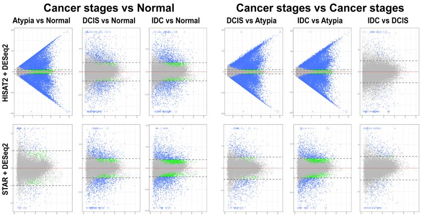
J. Pers. Med. 2019, 9, 18                                                                            2 of 18

has been embraced for its potential for precision medicine in diagnoses, prognoses, and therapeutic
decisions [2–4]. In comparison to the preceding popular technology for gene expression, microarrays,
RNA-seq provides substantially increased transcriptome coverage and is more amenable to discovery
science, as the identification of expressed loci or alternative splicing is not limited to the probes
present on the array [5,6]. At the same time, gene expression analysis becomes computationally
more challenging due to the requirement to correctly classify all sequence read outputs in RNA-seq
datasets. As “wet lab” NGS technologies and “dry lab” high performance computers supporting
NGS technology became more economical, RNA-seq and other NGS datasets expanded exponentially
producing massive amounts of data [7]. Many researchers and clinicians, who utilize RNA-seq in their
experiments, rely on outsourcing to cores or companies to generate and analyze their RNA-seq data.
This practice is common with many niche experiments, especially in “omics”-based studies.
     For an ideal RNA-seq experiment, researchers and clinicians would acquire freshly frozen tissue
samples with minimal inclusion of non-target tissues, such as blood and fat, the most common
contaminants. In reality, majority of clinical research relies on either archived tissue specimens, mainly
as formalin-fixed, paraffin-embedded (FFPE) biopsies, which have increased RNA degradation and
decreased poly(A) binding affinity [8–10], or punch biopsies for discrete tissue collection, which
severely limits sample material [11]. We analyzed RNA-seq data from bore-dissected samples from
FFPE breast tissue, which are known to be highly variable for quality and depth of sequencing
results. These transcriptome datasets correspond to the typical quality that biomedical researchers
will encounter using transcriptome studies for precision medicine, experiments, or re-analysis.
The most common experimental question addressed in RNA-seq transcriptome studies is identifying
differential expression among normal stages and stages of disease progression, and sometimes among
treatment groups, to pinpoint pathways and putative molecular mechanisms underlying disease or its
pathophysiology. To determine differential expression, RNA-seq reads need to be assessed for quality
and then aligned to a reference genome. This underscores the essential importance to investigate the
impacts of bioinformatics tools for sequence alignment and differential expression on accurate results
and interpretation of transcriptome studies collected from FFPE specimens, which was the goal of
our study. This paper also serves to point out the pragmatic shortcomings of universally applying a
rigid “standard operating procedure” set of bioinformatics tools to RNA-seq data, by demonstrating
the impacts and limitations of biological conditions, especially in sample processing and choice
of programs.
     We focused on two of the most popular sequence aligners, HISAT2 [12], and STAR [13], which
superseded the once ubiquitous TopHat aligner program because of their superior computational
speed. For differential expression, we used two differential gene expression testing tools, DESeq2 [14]
and edgeR [15]. According to citation reports, currently edgeR and DESeq2 are the leading programs
for RNA-seq data quantification and differential expression testing, with 10,013 and 8147 citations as of
22 February 2019 [16]. These popular bioinformatics tools are available for users via the open-source
Galaxy platform [17], a portal designed to support a wide range of researchers from those with little
or no experience or training, to professional bioinformaticians. We also investigated the strengths
and weaknesses of the two most widely used differential expression analysis tools and present a
straightforward bioinformatics pipeline from raw data to downstream analysis of gene expression,
suitable even for researchers with minimal bioinformatics expertise. We performed differential gene
expression analysis using the series of breast cancer progression RNA-seq data from micropunched
FFPE samples and assessed similarities and differences in the results to detect the effects of different
aligners upon read mapping affecting gene expression counts. Furthermore, we tested the impacts of
different algorithms used to detect differential gene expression upon the list of statistically significant
transcripts, as well as pathway analysis using Gene Ontology [18] enrichment.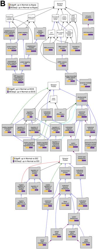
J. Pers. Med. 2019, 9, 18                                                                         3 of 18

2. Materials and Methods

2.1. Breast Cancer Samples
     RNA-seq data used in this study are publicly available (BioProject ID: PRJNA205694 [19]).
The dataset represents 72 RNA sequencing experiments from biopsies at different stages of breast
cancer: 24 normal tissue samples, 25 early neoplasias (Atypia), 9 ductal carcinomas in situ (DCIS) and
14 infiltrating ductal carcinomas (IDC), from 25 patients. Briefly, RNA was extracted from core punches
of FFPE specimens after histological confirmation of the cancer stage by board-certified pathologists
and only samples that possessed >90% of luminal cells with the appropriate diagnosis were used for
sequencing. Directional cDNA libraries were constructed and sequenced using Illumina GAIIx to
obtain 36-base single-end reads.

2.2. RNA-seq Reads Alignment
     We used two programs, STAR and HISAT2, which utilize different strategies to align the RNA-seq
reads to human genome assembly. To improve alignment accuracy, both programs use a dataset
of known splice sites to correctly identify potential spliced sequencing reads among RNA-seq data.
This dataset, in “gene transfer format” (gtf), was obtained from ENSEMBL (release 87, 12/8/2016).
Reads were aligned to the human reference genome assembly (hg19).

2.2.1. STAR
     STAR’s algorithm [13] uses a two-step approach. STAR aligns the first portion, referred to as
“seed”, for a specific read sequence output against a reference genome to the maximum mappable
length (MML) of the read. Next, STAR aligns the remaining portion, called the “second seed”, to its
MML. After the read is completely aligned, STAR joins the two or more “seeds” together and scores the
aligned reads based on a user-defined penalty for mismatches, insertions, and deletions. The joined
seeds with the highest score are chosen as the correct alignment for a specific read sequence output.
This approach allows for quick and easy annotation of multi-mapping reads with their own alignment
scores. In our analysis, STAR was used with the following parameters:
      –seedSearchStartLmax 50 –seedSearchStartLmaxOverLread 1.0 –seedSearchLmax 0 –seedMultimapNmax
      10000 –seedPerReadMax 1000 –seedPerWindowMax 50 –seedNonoLociPerWindow 10 –alignIntron
      Min 21 –alignIntronMax 0 –alignMatesGapMax 0 –alignSJoverhangMin 5 –alignSJDBoverhangmin 3
      –alignSpliceMateMapLmin 0 –alignSplicedMateMapeLminOverLmate 0.66 –alignWindowsPerReadN
      max 10000 –alignTranscriptsPerWindowNmax 100 –alignTranscriptsPerReadNmax 10000 –align
      EndsType Local

2.2.2. HISAT2
     HISAT2 uses the Bowtie2 [20] algorithm to construct and search Ferragina–Manzini (FM)
indices [21]. HISAT2 employs two types of indices for aligning: firstly, a whole-genome FM index
to anchor alignments and secondly, numerous overlapping local FM indices for alignment extension.
HISAT was used for our analysis with the following parameters:
      –mp MX=6, MN=2 –sp MX=2,MN=1 –np 1 –rdg 5,3 –rfg 5,3 –score-min L,0,-0.2 –pen-cansplice
      0 –pen-noncansplice 12 –pen-canintronlen G,-8,1 –pen-noncanintronlen G,-8,1 –min-intronlen 20
      –max-intronlen 500000

2.3. Gene Expression Counts
      The simplest method for estimating transcript expression is to count the raw reads for each
annotated gene locus in the genome assembly. This approach uses a gtf file containing genomic
coordinates, such as gene nomenclature, positions in the chromosome for each exon, transcription start
site, transcription termination site, etc. We used FeatureCounts [22], to extract information from the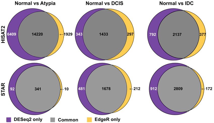
J. Pers. Med. 2019, 9, 18                                                                           4 of 18

binary format for storing sequencing data, i.e., BAM files reads overlapping with genomic features
in an input gtf file containing exon coordinates for all transcripts in the genome assembly using the
following parameters: –t ‘exon’ –g ‘gene_id’ –M –fraction –Q 12 –minOverlap 30.

2.4. Data Normalization and Quality Control

2.4.1. Data Normalization
    To account for the depth of sequencing impacts, which affect read numbers of individual transcripts,
we use normalized expression data, specifically counts per million (CPM) [23], to perform quality
comparison of datasets. To calculate CPM values, we used the following formula:

                                       CPMi = Ri /TRa × 1,000,000                                      (1)

where CPMi is a CPM value of a gene in a biological replicate; Ri is the number of reads mapping to all
exons of this gene in this biological replicate; TRa is the total number of reads aligned (anywhere in the
genome) from this biological replicate (i.e., the number of aligned reads in either STAR or HISAT2
output “binary alignment map” bam files). This procedure also transforms data from counts to a
continuous scale.

2.4.2. Quality Control
      For quality control, we used ClustVis [24], a statistical tool for clustering of complex data such
as RNAseq, based on principal component analysis and visualization of results. Any samples that
fell outside of the initial 95% confidence interval on the two-dimensional PCA plot were flagged as
outliers and removed before further analysis. ClustVis [24] has an intuitive user interface and was built
using several R software packages to provide Principal Component Analysis and heat map plots of
high-dimensional data from a data matrix. Data may be uploaded as text file, or manually entered into
ClustVis text box. Rows (e.g., genes) and columns (e.g., samples) may contain multiple annotations to
be detected automatically, or input manually, to provide additional features (e.g., color for groups,
confidence intervals) applied to the PCA and heat map plots.

2.5. Differential Gene Expression Analysis
      Both tools are R packages and require raw read counts in a data matrix, which are normalized to
account for differences in sequencing depth, and low count variability. Both tools assume RNA-seq
data display overdispersion with variance greater than expected for random sampling. Both programs
also assume RNA-seq data conform to a negative binomial distribution and employ Bayesian methods
to fit raw gene expression counts into this distribution. To display differential expression outputs
uniformly, we used the R software package Visualization of Differential Gene Expression using R
(ViDGER) [25].

2.5.1. DESeq2
    This program, DESeq2, was used to detect differential expression in RNA-seq data. DESeq2
normalizes the counts of each gene employing a generalized linear model [26]. Afterwards, DESeq2 uses
an empirical Bayes shrinkage to detect and correct for dispersion and log2 -fold change (LFC) estimates.

2.5.2. edgeR
     The other popular program to detect differential expression, edgeR, uses a default method
of normalization called trimmed mean of M-values, (TMM), which is obtained with the function:
calcNormFactors. This method of normalization estimates the ratio of RNA production through a
weighted trimmed mean of the log expression ratios. There are alternative normalization methods
J. Pers. Med. 2019, 9, 18 5 of 18
available in edgeR to account for data that fail to conform to a negative binomial distribution, which is
assumed with TMM. To control for false discovery rate (FDR) we applied the estimateDisp function.
J. Pers. Med. 2019, 9, 18 5 of 18
2.6. Gene Enrichment Analysis Using Visual Annotation Display (VLAD)
2.6. Gene Enrichment Analysis Using Visual Annotation Display (VLAD)
VLAD [27], accessible via Mouse Genome Informatics (MGI) web portal, is a powerful tool to find
VLAD [27],themes
common functional accessible via Mouse
in the lists of Genome
genes byInformatics
analyzing (MGI) web over-
statistical portal,orisunderrepresentation
a powerful tool to of
ontological annotations. Currently, users can choose among Gene Ontology (GO) [18]over‐
find common functional themes in the lists of genes by analyzing statistical or
annotations
underrepresentation of ontological annotations. Currently, users can choose among
for human genes, Gene Ontology, and Mammalian Phenotype Ontology (MP) [28] annotations for Gene Ontology
(GO) [18] annotations for human genes, Gene Ontology, and Mammalian Phenotype Ontology (MP)
mouse genes, or upload a file of own annotations (in open biomedical ontology [29] “obo” format).
[28] annotations for mouse genes, or upload a file of own annotations (in open biomedical ontology
Unlike other packages for ontological enrichment, VLAD uniquely allows simultaneous analysis and
[29] “obo” format). Unlike other packages for ontological enrichment, VLAD uniquely allows
visualization of more
simultaneous than
analysis andone query (i.e.,
visualization of several
more thanlists
oneofquery
genes may
(i.e., be analyzed
several andmay
lists of genes visualized
be
simultaneously),
analyzed andas well as permits
visualized a user toasprovide
simultaneously), well as own “universe
permits a user toset”, i.e., own
provide gene“universe
list to testset”,
queries.
i.e., gene list to test queries.
3. Results
3. Results
3.1. Bioinformatics Pipeline and Quality Control
3.1. Bioinformatics Pipeline and Quality Control
RNA-seq data were analyzed using two different read aligners, STAR and HISAT2, to compare
RNA‐seq
potential impacts of data were
read analyzedtousing
mapping two different
the genome read aligners,
assembly upon the STAR and HISAT2,
ultimate outputstoof
compare
differential
potential impacts of read mapping to the genome assembly upon the ultimate outputs of
gene expression. Briefly, RNA-seq output reads were aligned to the genome assembly (hg19) by either differential
geneorexpression.
HISAT2 STAR, reads Briefly,
mappedRNA‐seq output
to genes werereads were aligned
counted for eachtoindividual
the genome assembly
gene (hg19)
to yield raw bycounts,
either HISAT2 or STAR, reads mapped to genes were counted for each individual gene to yield raw
subsequently count data were normalized, assessed for quality control using Principal Component
counts, subsequently count data were normalized, assessed for quality control using Principal
Analysis using ClustVis, and sample outliers removed before performing differential gene expression
Component Analysis using ClustVis, and sample outliers removed before performing differential
analysis by two different programs, edgeR and DESeq2, to identify significant gene expression changes
gene expression analysis by two different programs, edgeR and DESeq2, to identify significant gene
acrossexpression
breast cancer stages
changes (Figure
across breast 1).
cancer stages (Figure 1).
Figure
Figure 1. Bioinformatics
1. Bioinformatics pipelineemployed
pipeline employed to
to test
test differences
differencesininaligners andand
aligners differential expression
differential expression
programs. RNA‐seq: RNA sequencing.
programs. RNA-seq: RNA sequencing.
To eliminate
To eliminate sample
sample outlier
outlier biases,we
biases, weperformed
performed Principal
PrincipalComponent
Component Analysis (PCA)
Analysis of gene
(PCA) of gene
expression counts for each sample by each stage for both aligners. Gene
expression counts for each sample by each stage for both aligners. Gene expression counts expression counts werewere
collected using featureCounts and normalized to the total number of aligned reads for each sample,
collected using featureCounts and normalized to the total number of aligned reads for each sample,
and PCA completed on these data using ClustVis large edition (Figure 2). For all subsequent analysis,
and PCA completed on these data using ClustVis large edition (Figure 2). For all subsequent analysis,
any samples that fell outside the 95% confidence ellipse in their respective stages (Normal, Atypia,
any samples
DCIS, andthat
IDC)fell outside
were the For
removed. 95%bothconfidence
HISAT2 andellipse
STAR,in the
their respective
same stages
samples fell (Normal,
outside of the 95%Atypia,
DCIS,confidence
and IDC)ellipse
were removed. ForIn
in each stage. both HISAT2
total, and STAR,
we identified the same
six outlier samples
samples in thefell outside
RNA‐seq of the 95%
dataset,
confidence ellipse
which were: in each stage.
SRX286949 (normalIn total,SRX286945
tissue), we identified six outlier(atypia),
and SRX286964 samples in the RNA-seq
SRX286961 dataset,
(DCIS), and
whichSRX286951
were: SRX286949 (normalAtypia
(IDC). Overall, tissue), SRX286945
stage and
presented SRX286964
more (atypia),
heterogeneity thanSRX286961
any other(DCIS),
stage, and
irrespective
SRX286951 (IDC). ofOverall,
the aligner. Unexpectedly,
Atypia the PCAmore
stage presented plotsheterogeneity
for all stages inthan
HISAT2
anydata clustered
other atypia
stage, irrespective
stage samples separately from all other stages (Figure 2A), which didn’t occur in
of the aligner. Unexpectedly, the PCA plots for all stages in HISAT2 data clustered atypia stage PCA plots for STAR
samples
data (Figure 2B).
separately from all other stages (Figure 2A), which didn’t occur in PCA plots for STAR data (Figure 2B).J. Pers. Med. 2019, 9, 18 6 of 18
J. Pers. Med. 2019, 9, 18 6 of 18
J. Pers. Med. 2019, 9, 18 6 of 18
Figure 2.
Figure 2. Principal
Figure Principal
Component
2. Principal Component Analysis
Analysis
Component (PCA)visualization
(PCA)
Analysis (PCA) visualization of
visualization of gene
gene expression
of gene data from
expression
expression data fromdata
HISAT2
from HISAT2
HISAT2
and
and STAR
STAR alignments.
alignments. Clustering
Clustering of
of samples
samples on
on HISAT2
HISAT2 (A)
(A) and
and STAR
STAR (B)
(B) on
on the
the first
first two
two principal
principal
and STAR alignments. Clustering
components before
of samples on HISAT2 (A) and STAR (B) on the first two principal
components before outlier
outlier removal.
removal.
components before outlier removal.
3.2. Outputs of Aligners
3.2. Outputs of Aligners
All reads for all samples were aligned to the human genome assembly (hg19). Overall, STAR
3.2. Outputs of Aligners
All reads
significantly for all samples
outperformed wereinaligned
HISAT2 aligningtothe
the human
FASTQ genome
reads to theassembly (hg19).3).Overall,
genome (Figure STAR
The generally
significantly
low proportion outperformed
of alignedwere HISAT2
reads to all in aligning
input reads the both
for FASTQ reads is
programs tolikely
the genome (Figure
due to the quality3).ofOverall,
The
the
All reads for all
generally low
samples
proportion of
aligned
aligned reads
to
to
theinput
all
human
reads
genome
for both
assembly
programs is
(hg19).
likely due to the
STAR
libraries, as a significant number of input reads were poly(A) sequences, Illumina adapter sequences,
significantlyquality
outperformed HISAT2
of the libraries, in aligning
as a significant number the FASTQ
of input reads
reads were to the
poly(A) genome
sequences, (Figure 3). The
Illumina
and reads corresponding to the very 30 -ends of mRNAs, which are too uninformative for correct
generally lowadapter sequences,ofand
proportion reads corresponding to the very 3’‐ends of mRNAs, which are too
aligned
mapping (Supplemental Table S1).reads to all input reads for both programs is likely due to the
uninformative for correct mapping (Supplemental Table S1).
quality of the libraries, as a significant number of input reads were poly(A) sequences, Illumina
adapter sequences, and reads corresponding to the very 3’‐ends of mRNAs, which are too
uninformative for correct mapping (Supplemental Table S1).
PerformanceofofHISAT2
Figure 3. Performance HISAT2and
andSTAR
STAR aligners
aligners onon
thethe breast
breast cancer
cancer series
series data.
data. p < ***
* pJ. Pers. Med. 2019, 9, 18 7 of 18
came from 384 and 366 genes for STAR and HISAT2, respectively, and the lists shared 319 of those
genes. The
J. Pers. Med.
high
2019,
amount of discrepancies in atypia convinced us to investigate the underlying7 factors
J. Pers. Med. 2019, 9, 9,
1818 of7 18
of 18
resulting in the major differences in alignment.
Figure
Figure 4. Overlap
4. Overlap between
between thethe highest
highest expressed
expressed genesgenes in breast
in the the breast
cancercancer datasets
datasets aligned
aligned by
by HISAT2
Figure 4. Overlap
or STAR.between the highest expressed genes in the breast in cancer datasets aligned by
or HISAT2 HISAT2‐identified
STAR. HISAT2-identified genes are ingenes are in genes
red; STAR red; STAR
are ingenes
green;are green; overlapping
overlapping genes are ingenes
yellow.
HISAT2 or STAR.
are in yellow. HISAT2‐identified genes are in red; STAR genes are in green; overlapping genes
3.3.2.are
Alignment
in yellow.to Pseudogenes
3.3.2. Alignment to Pseudogenes
Processed pseudogenes, sometimes referred to as non-functional retrogenes, are intronless gene
3.3.2. Alignment to Pseudogenes
copies Processed
producedpseudogenes, sometimes referred
by reverse transcription to as non‐functional
of an original “parent” gene retrogenes,
mRNA are andintronless
insertiongene of the
Processed
copies
resulting cDNApseudogenes,
produced by reverse
copy elsewhere sometimesin the referred
transcription toProcessed
as non‐functional
of an original
genome. “parent” generetrogenes,
pseudogenesmRNA areand are intronless
insertion
non-functional gene
of theand
copies produced
resulting cDNA by reverse
copy transcription
elsewhere in the of an
genome. original “parent”
Processed gene
pseudogenes
comprise the bulk of the known loci in the broad category of “pseudogenes”, i.e., genomic loci mRNA
are and insertion
non‐functional of
and the
comprise
resulting the
cDNA bulk
copy of the known
elsewhere inloci
the in the
genome. broad category
Processed of “pseudogenes”,
pseudogenes
harboring similarity to a protein-coding gene but not having any recognized biological function. are i.e., genomic
non‐functional loci
and
Theharboring
comprise thesimilarity
sequence bulk of tothe
similarity aamong
protein‐coding
known loci ingene
processed the but not having
broad
pseudogenes andany
category ofrecognized
their biological
“pseudogenes”,
parent genes function.
i.e.,
poses agenomic
problem Theloci
for
sequence
harboring similarity
similarity toamong
a processed
protein‐coding pseudogenes
gene but not and
havingtheirany parent genes
recognized
aligners, whose algorithms have to decide when assigning a read to a particular locus in the genome. poses
biologicala problem
function. for
The
aligners,similarity
sequence whose algorithms
among have to decide
processed when assigning
pseudogenes andatheir
read to a particular
parent genes locus
posesin athe genome.for
problem
To determine the underlying factors causing the different alignments, we analyzed the numbers
To determine
aligners, the underlying
whose algorithms factors
have toby causing
decide when the different
assigning alignments,
a read to the we analyzed
a particular the numbers
locustested,
in the genome. of
of reads mapped to pseudogenes HISAT2 and STAR. Between two aligners HISAT2
reads mapped
To determinehad to pseudogenes
thesignificantly
underlying factors by HISAT2 and STAR. Between the two aligners tested, HISAT2
consistently higher causing
amountsthe of different alignments,
reads aligned we analyzed
to pseudogenes when thecompared
numbers to of
consistently
reads (Figure had
mapped5A). significantly
to pseudogenes higher amounts of reads aligned to pseudogenes when compared to
STAR Furthermore,by forHISAT2
Atypia stage,and STAR.
HISAT2 Between the two higher
had drastically aligners tested, of
amounts HISAT2
reads
STAR (Figure 5A). Furthermore, for Atypia stage, HISAT2 had drastically higher amounts of reads
consistently had significantly higher amounts of reads aligned to
aligned to pseudogenes than the other stages. To determine what portion of the top 50% of mapped pseudogenes when compared to
aligned to pseudogenes than the other stages. To determine what portion of the top 50% of mapped
STAR
reads (Figure
were 5A).
pseudogenes,Furthermore, for Atypia stage, HISAT2 had drastically higher amounts of reads
reads were pseudogenes,we weobtained
obtainedaalist list of
of pseudogenes
pseudogenes from fromthe thehg19
hg19gtf
gtfannotation
annotation filefile
wewe usedused
aligned
and to pseudogenes
compared this list thanthe
with thetop other 50% stages.
of To determine
mapped genes what
for each portion
stage of the
and eachtopaligner.
50% of A mapped
single
and compared this list with the top 50% of mapped genes for each stage and each aligner. A single
reads were pseudogenes,
pseudogene was we obtained a list of pseudogenes from thethe hg19 gtf annotation filereads
we used
pseudogene wasininthe thegenegenelist
listfor
foreach
each stage
stage which represented
which represented top50%
the top 50% ofofmapped
mapped reads forfor
and
STAR. compared
STAR.
this
Conversely,
Conversely,
list
HISAT2with the
HISAT2consistently
top 50%
consistentlyhad
of mapped
had higher
genes
amountsof
higher amounts
for each stage
ofpseudogenes and each
pseudogenesrepresented aligner.
represented in in
A single
thethe
toptop
pseudogene
50% of mapped was in
reads the gene
(Figure
50% of mapped reads (Figure 5B). list
5B). for each stage which represented the top 50% of mapped reads for
STAR. Conversely, HISAT2 consistently had higher amounts of pseudogenes represented in the top
50% of mapped reads (Figure 5B).
Figure
Figure 5. 5.Expression
Expressionof ofpseudogenes
pseudogenes ininHISAT2
HISAT2and andSTAR
STAR alignment
alignment data. A: Percent
data. of all of
(A) Percent reads, by
all reads,
bystage,
stage,aligned
alignedtotoannotated
annotatedpseudogene
pseudogeneloci locibybyHISAT2
HISAT2(red)(red)andandSTAR
STAR(green).
(green).B:(B)
Number
Number of of
retrogenes among highest-expressed genes by stage and aligner. ** p < 0.01, *** p < 0.001, 2-tailed t-tests
retrogenes among highest‐expressed genes by stage and aligner. ** p < 0.01, *** p < 0.001, 2‐tailed t‐
Figure 5. 2Expression of pseudogenes in HISAT2 and STAR alignment data. A: Percent of all reads, by
(5A), or χ tests (5B). DCIS: ductal carcinoma in situ; IDC: infiltrating ductal carcinoma.
tests (5A), or χ2 tests (5B). DCIS: ductal carcinoma in situ; IDC: infiltrating ductal carcinoma.
stage, aligned to annotated pseudogene loci by HISAT2 (red) and STAR (green). B: Number of
3.4.retrogenes
Differential among highest‐expressed
Gene Expression Analysisgenes by stage and aligner. ** p < 0.01, *** p < 0.001, 2‐tailed t‐
tests (5A), or χ2 tests (5B). DCIS: ductal carcinoma in situ; IDC: infiltrating ductal carcinoma.
The differential expression comparison on data from different alignment tools was done to
further explore
3.4. Differential the Expression
Gene consequences of previously described alignment tool biases, as well as to compare
Analysis
The differential expression comparison on data from different alignment tools was done to
further explore the consequences of previously described alignment tool biases, as well as to compareJ. Pers. Med. 2019, 9, 18 8 of 18
3.4. Differential Gene Expression Analysis
The differential expression comparison on data from different alignment tools was done to further
J. Pers. Med. 2019, 9, 18
explore the consequences of previously described alignment tool biases, as well as to compare8the
of 18
two
popular tools used for the purpose of identification and quantification of gene expression differences
the two popular tools used for the purpose of identification and quantification of gene expression
between conditions,
differences betweenedgeR and DESeq2.
conditions, edgeR and DESeq2.
3.4.1. edgeR Following HISAT2 or STAR
3.4.1. edgeR Following HISAT2 or STAR
Overall
Overall patterns
patternsofofdifferential
differentialgene
gene expression performedby
expression performed byedgeR
edgeRononHISAT2
HISAT2 oror STAR
STAR data
data
were similar for all pairwise stage comparisons, except atypia versus any other stage
were similar for all pairwise stage comparisons, except atypia versus any other stage (Figure 6).(Figure 6). HISAT2
consistently had the atypia
HISAT2 consistently had stage comparisons
the atypia produce >15,000
stage comparisons producestatistically significant differentially
>15,000 statistically significant
expressed transcripts
differentially withtranscripts
expressed log2 foldwith
change fold ≥1
log2LFC change LFC≤−1
or LFC ≥1 or(i.e.,
LFC at≤‐1
least two-fold
(i.e., at least increase
two‐fold or
decrease in transcript expression levels between stages) (Figure 6, top panels). Conversely,
increase or decrease in transcript expression levels between stages) (Figure 6, top panels). Conversely, differential
expression pairwise
differential comparisons
expression pairwisewith STAR atypia
comparisons stage
with versus
STAR eachstage
atypia other versus
stage identified
each other350stage
to 2496
differentially expressed
identified 350 genes (Figureexpressed
to 2496 differentially 6, bottomgenes
panels).
(Figure 6, bottom panels).
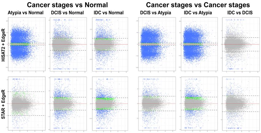
Figure Mean-average
6. 6.
Figure Mean‐average(MA) (MA)plots
plotsofof pairwise comparisonsofofall
pairwise comparisons allstages
stagesusing
using edgeR.
edgeR. HISAT2
HISAT2 (top)
(top)
andand STAR
STAR (bottom)
(bottom) gene
gene counts
counts to identify
to identify differentially
differentially expressed
expressed genes.
genes. Each
Each gene
gene is represented
is represented by a
by adot.
single single
Bluedot. Blue
dots dots represent
represent genes withgenes with significant
significant expression
expression difference
difference and LFCand ≥ 1.LFC≥1. Blue
Blue triangles
trianglesgenes
represent represent genes withexpression
with significant expressionand
significantdifference difference and
LFC is off LFCGreen
scale. is offdots
scale. Green dots
represent genes
with significant expression difference but LFC < 1; grey dots represent statistically non-significant
represent genes with significant expression difference but LFC LFC
having 1 and>1177
and 177 with
genes genes
LFC < 1 in
with LFC 1, 482 LFC < 1, and
comparisons. Normal versus DCIS and Normal versus IDC analysis revealed 1677 LFC >1, 482 LFC
2304
1, 1417 LFC 1, 1417 LFC < 1 differentially expressed genes, respectively (Figure 7, bottom panels). Similarly bottom
panels).differential
to edgeR, Similarly to edgeR, differential
expression analysis ofexpression
HISAT2 withanalysis
DESeq2of HISAT2 withproduced
consistently DESeq2 consistently
high numbers
produced high numbers of statistically significant differentially expressed genes
of statistically significant differentially expressed genes in atypia pairwise comparisons, in atypia pairwise
>19,000 genes
comparisons, >19,000 genes with LFC >1 (Figure 7, top panels). Normal versus Atypia, Normal versus
with LFC > 1 (Figure 7, top panels). Normal versus Atypia, Normal versus DCIS, and Normal versus
DCIS, and Normal versus IDC analysis revealed 19,419 LFC >1, 1212 LFC 1, 190 LFC
IDC analysis revealed 19,419 LFC > 1, 1212 LFC < 1, 1585 LFC > 1, 190 LFC < 1, and 2196 LFC > 1, 732
< 1, and 2196 LFC >1, 732 LFCJ. Pers. Med. 2019, 9, 18 9 of 18
J. Pers. Med. 2019, 9, 18 9 of 18
J. Pers. Med. 2019, 9, 18 9 of 18
Figure
Figure 7. Mean‐average
7. 7.
Figure Mean‐average(MA)
Mean-average (MA)plots
(MA) plotsof
plots ofpairwise
of pairwise comparisons
pairwise comparisonsof
comparisons of all
ofall stages
allstages using
stagesusing DeSeq2.
usingDeSeq2.
DeSeq2. HISAT2
HISAT2
HISAT2 (top)
(top)
(top)
and
and STAR
STAR
and STAR (bottom)
(bottom) gene
(bottom)gene counts
genecounts
countsforfor all
forall samples
allsamples were analyzed
samples were analyzed to
analyzed toidentify
to identifydifferentially
identify differentially
differentially expressed
expressed
expressed
genes.
genes. Each
genes. Each
Each gene
gene
gene is
isisrepresented
representedby
represented byaaasingle
by single dot.
single dot. Blue
dot. Blue dots
Blue dots represent
dotsrepresent genes
representgenes with
geneswith significant
withsignificant
significant expression
expression
expression
difference
difference and
difference
and andlog2‐fold change
log2‐foldchange
log2-fold (LFC) ≥
(LFC)≥≥ 1.
change(LFC) 1. Blue triangles
1. Blue triangles represent
trianglesrepresent genes
representgenes with
geneswith significant
withsignificant
significant expression
expression
expression
difference
difference and
difference
and andLFC
LFC
LFC isisoff
is off scale.
scale.Green
offscale. Greendots
Green dots represent
dots genes
represent genes
represent with
genes with significant
withsignificant expression
significantexpression
expression difference
difference
difference but
butbut
LFC
LFCLFC< 1;
< 1; grey
< 1; grey
grey dots
dots
dots represent statistically
representstatistically
represent non‐significant
statisticallynon-significant genes. Y‐axis
non‐significant genes.
genes. Y‐axis(all
Y-axis (allplots):
(all plots):log
plots): log
log 2 of
2 of expression
expression
2 of expression
fold
fold
fold change;
change;
change; X‐axis
X‐axis
X-axis (allplots):
(all
(all plots):log
plots): log ofmean
log222of
of mean value
mean value of
value of gene
geneexpression
gene expressionacross
expression acrossallall
across allstages.
stages.
stages.
3.4.3. Comparison
3.4.3.
3.4.3. ofofDESeq2
Comparisonof
Comparison DESeq2 and
DESeq2and edgeR
andedgeR Results
edgeRresults
results
The
TheThe
totaltotal
total number
number
number ofof statistically
statistically
of statistically significant
significant differentially
differentially
significant expressed
differentially expressed genes
genesincomparisons,
genes in pairwise
expressed inpairwise
pairwise
by comparisons,
aligner andby
comparisons, by alignerand
differential
aligner and differential
expression expression
tool,expression
differential tool,
tool, is
is summarized insummarized
is ininFigure
Figure 8. Overall,
summarized 8.8.
DESeq2
Figure Overall, DESeq2
produced
Overall, more
DESeq2
produced
inflated lists more inflated
comparing tolists comparing
edgeR.
produced more inflated lists comparing to edgeR. to edgeR.
Figure 8. Total number of differentially expressed genes in pairwise comparisons, by aligner (HISAT2
or STAR),
Figure and
Total
8. Total quantification
number of program expressed
of differentially
differentially (edgeR or DESeq2). (HISAT2
genes in pairwise comparisons, by aligner (HISAT2
or STAR), and quantification program (edgeR or DESeq2).
and quantification program (edgeR or DESeq2).
Next, to compare how similar these most common differential gene expression analysis tools,
edgeR
Next,and
Next, to DESeq2, calculate
to compare
compare how expression
how similar
similar differences
these most
these most common
common ondifferential
the same data,
differential genewe
gene comparedanalysis
expression
expression lists of tools,
analysis all
tools,
differentially
edgeR
edgeR and expressed
and DESeq2, genes generated
calculate expression
DESeq2, calculate by these programs
expression differences
differences on
on the and produced
the same
same data, Venn diagrams,
we compared
data, we compared listsfor each
lists of
of all
all
pairwise cancer
differentially stage comparison
expressed genes to normal
generated by samples.
these DESeq2
programs andand edgeR shared
produced Venn 14,220, 1433,
diagrams, forand
each
differentially expressed genes generated by these programs and produced Venn diagrams, for each
2137 of the differentially
pairwise expressed genes on the HISAT2DESeq2
alignment pairwise
edgeRcomparisons for Normal
pairwise cancer
cancer stage
stage comparison
comparison toto normal
normal samples.
samples. DESeq2 and and edgeR shared 14,220,
shared 14,220, 1433,
1433, and
and
versus
2137 of Atypia,
the Normal
differentially versus
expressed DCIS,
genes and
on Normal
the versus
HISAT2 IDC,
alignment respectively
pairwise (Figure
comparisons 9, top
for row).
Normal
2137 of the differentially expressed genes on the HISAT2 alignment pairwise comparisons for Normal
versus Atypia, Normal versus DCIS, and Normal versus IDC, respectively (Figure 9, top row).J. Pers. Med. 2019, 9, 18 10 of 18
J. Pers. Med. 2019, 9, 18
versus Atypia, Normal versus DCIS, and Normal versus IDC, respectively (Figure 9, top row).10Notably, of 18
at the Atypia stage, HISAT2 yielded a disproportionally high amount of differentially expressed
Notably, at the Atypia stage, HISAT2 yielded a disproportionally high amount of differentially
genes detected by both edgeR and DESeq2 programs (14,220 common genes, 6409 DESeq2 only,
expressed genes detected by both edgeR and DESeq2 programs (14,220 common genes, 6409 DESeq2
and 1929 edgeR only; Figure 9 top left panel), reflecting the global RNA-seq data misalignment to
only, and 1929 edgeR only; Figure 9 top left panel), reflecting the global RNA‐seq data misalignment
processed pseudogenes
to processed pseudogenes by HISAT2
by HISAT2 (Figures 4–7).
(Figures 4–7).DESeq2
DESeq2andand edgeR shared341,
edgeR shared 341,1678,
1678,and
and 2809
2809
of the
of thedifferentially
differentially expressed
expressedtranscripts
transcriptson
onthe
the STAR
STAR alignment pairwisecomparisons
alignment pairwise comparisonsforfor Normal
Normal
versus Atypia, Normal versus DCIS, and Normal versus IDC, respectively (Figure
versus Atypia, Normal versus DCIS, and Normal versus IDC, respectively (Figure 9, bottom row). 9, bottom row).
Overall,
Overall, STAR
STARalignment
alignmentyielded
yieldedthe
the highest
highest percent of overlapping
percent of overlappinggenes
genesbetween
betweendifferential
differential
expression
expression programs.
programs.
Figure Overlap
9. 9.
Figure Overlapamong
amonggenes
genesidentified
identified as
as differentially expressedby
differentially expressed byeither
eitherDESeq2
DESeq2oror edgeR
edgeR in in
HISAT2
HISAT2 or or STAR‐aligned
STAR-aligned RNA‐seqdata.
RNA-seq data.
3.4.4. Downstream
3.4.4. Analysis
Downstream AnalysisofofGene
GeneExpression
Expression
ToTo testtest
if if
downstream
downstreamanalysis
analysis of
of differentially
differentially expressed genesisisaffected
expressed genes affectedbybythe
thetype
type
of of
software
softwareused usedtoto
identify
identifythese
thesegenes,
genes,wewe performed
performed Gene Ontologyenrichment
Gene Ontology enrichmentstudies
studies with
with thethe
Visual Annotation
Visual AnnotationDisplay
Displaytool
tool(VLAD)
(VLAD)forfor genes
genes found
found significantly downregulatedininpairwise
significantly downregulated pairwise
comparisons
comparisons ofofcancer
cancerstages
stages(Atypia,
(Atypia, DCIS,
DCIS, IDC)
IDC) to normal
normal samples
samplesby byeach
eachprogram
program (DESEq2,
(DESEq2,
edgeR), using gene expression data only from STAR alignments because of the global
edgeR), using gene expression data only from STAR alignments because of the global misalignment to misalignment
to pseudogenes
pseudogenes by HISAT2.
by HISAT2. TheThe pathways
pathways representedininthe
represented theGO
GO category
category Molecular
MolecularFunction,
Function, with
with
data
data from
from expression
expression significantlydecreased
significantly decreased inin DCIS
DCIS or
or IDC
IDC compared
comparedtotonormal
normalsamples,
samples, indicate
indicate
phosphatidylinositolkinase
phosphatidylinositol kinasepathways
pathways (Figure
(Figure 10A),
10A), which
which corroborate
corroboratethe thepreviously
previouslypublished
published
work on this dataset. Our analysis extends these previous findings because weprovide
work on this dataset. Our analysis extends these previous findings because we provideevidence
evidence of of
fundamental developmental pathways being decreased across all stages compared to normal
fundamental developmental pathways being decreased across all stages compared to normal samples
samples (Figure 10B). In addition, significant decrease of extracellular matrix genes, such as basement
(Figure 10B). In addition, significant decrease of extracellular matrix genes, such as basement membrane,
membrane, was found in cancer stages comparing to normal (Figure 10C). Overall, there was high
was found in cancer stages comparing to normal (Figure 10C). Overall, there was high concordance
concordance among overrepresented Gene Ontology terms identified among either DESeq2 or
among overrepresented Gene Ontology terms identified among either DESeq2 or edgeR-identified genes
edgeR‐identified genes significantly downregulated in cancer (Supplemental Table S2). Similar
significantly downregulated in cancer (Supplemental Table S2). Similar concordance in significantly
concordance in significantly enriched GO terms between DESeq2 or edgeR‐identified genes was
enriched
observedGOfor terms
genesbetween DESeq2
upregulated or edgeR-identified
in cancer (SupplementalgenesTablewas
S3). observed for genes upregulated in
cancer (Supplemental Table S3).J. Pers. Med. 2019, 9, 18 11 of 18
J. Pers. Med. 2019, 9, 18 11 of 18
Figure 10. Overrepresented Gene Ontology terms
Figure among genes upregulated in normal samples
10. Cont.
comparing to cancer stages. (A): Molecular Function, (B): Biological Process, and (C): Cellular
Component Gene Ontology (GO) categories; Top to bottom: Atypia versus Normal, DCIS versus
Normal and IDC versus normal comparisons. Significant GO terms are shaded; Size of the bar
represents significance of p‐value, and p‐value ratios between edgeR and Deseq2.J. Pers. Med. 2019, 9, 18 12 of 18
J. Pers. Med. 2019, 9, 18 12 of 18
Figure
Figure 10.10. Cont.
Continued.J. Pers. Med. 2019, 9, 18 13 of 18
J. Pers. Med. 2019, 9, 18 13 of 18
Figure 10. Overrepresented Gene Ontology Figureterms among genes upregulated in normal samples
10. Continued.
comparing to cancer stages. (A) Molecular Function, (B) Biological Process, and (C) Cellular Component
Gene Ontology (GO) categories; Top to bottom: Atypia versus Normal, DCIS versus Normal and IDC
versus normal comparisons. Significant GO terms are shaded; Size of the bar represents significance of
p-value, and p-value ratios between edgeR and Deseq2.J. Pers. Med. 2019, 9, 18 14 of 18
4. Discussion
Personalized medicine is a data science approach that promises focused treatments based on
an individual’s sequenced genome to precisely target pathways underlying disease or its symptoms.
To date only a few genotypes are robustly identified in breast cancer [30], such as BRCA1 and BRCA2,
which is inadequate to achieve the full promise of personalized medicine. A promising alternative to this
genetic approach to personalized medicine is transcriptome-based identification of altered pathways of
the diseased tissue to target its underlying disrupted cellular and molecular machinery. Identification
of affected pathways using bioinformatics pipelines for RNA-seq data empowers clinicians to make
a focused and informed decision on specific altered genes and pathways as potential therapeutic
targets in precision medicine for individual patients. The goal of our studies was to unveil potential
hidden biases arising from different bioinformatics analysis pipelines, and to find practical solutions
to circumvent and mitigate these biases that impact the downstream analyses in transcriptomics
experiments. Our results indicate that STAR and edgeR are robust and well-suited bioinformatics
tools for transcriptomics pipelines of the most commonly used clinical specimens, biopsies from FFPE
tissues, to precisely and accurately align and detect differential gene expression.
After initial quality control checks on the raw output from the sequencer, alignment is the first
step in RNA-seq analysis and all subsequent analysis relies profoundly upon this initial step [31].
Typically, reads obtained from sequencing will be mapped and aligned to a reference genome, which
is particularly prone to errors for RNA-seq data because of the presence of output reads spanning
exon-exon splice junctions. The most common software platforms available for mapping to a reference
genome, TopHat [32], HISAT2 [12], and STAR [13], identify splice junctions. These platforms differ in
computational speed and memory usage, and in their algorithms for handling base and splice junction
alignment precision. TopHat is currently becoming obsolete and has been superseded by HISAT2 due
to relative computational inefficiency. TopHat and HISAT2 are built on the short read mapping program
Bowtie2 [20]. While all three aligners are considered fast, HISAT2 and STAR consistently outperform
TopHat with respect to computational speed [13,33,34]. Although all three aligners performed well
in aligning a read onto the respective genomic locus, notable discrepancies and deficiencies were
found for TopHat yielding insufficient genomic mapping for reliable downstream analysis. Given
these reasons, and the fact that TopHat performance has been evaluated previous [34,35], our studies
assessed the alignment performance between STAR and HISAT2.
The next step in bioinformatics pipelines, quantification of gene expression, is commonly
performed with DESeq2 or edgeR programs [14,15]. A common drawback during this step is that
difference in sequencing depth between samples or groups by itself can skew results when estimating
differences in gene expression levels. The relative expression level of genes is often estimated based
on the number of mapped reads. These counts are subjected to statistical tools to assess significant
differences between groups. However, there is much confusion in the literature when reporting relative
expression level units in RNA-seq data. The confusion stems from the different forms of normalization
required for within versus between sample comparisons. Many methods for within sample comparison
attempt to correct for sequencing depth and gene length. These methods produce the most frequently
reported unit of expressions for RNA-seq data, which are read per kilobase of exon per million reads
(RPKM), fragments per kilobase of exon per million of reads (FPKM), and transcripts per million
(TPM) [36]. The order in which RPKM and FPKM normalize the read counts causes differences within
samples that should not be ignored. Instead, when comparing within samples one should use TPM
values which eliminates the invariance [36]. A relationship among RPKM, FPKM, and TPM is further
discussed elsewhere [37]. In this study, to account for the impact of sequencing depth, we normalized
expression data to counts per million (CPM) [23], which equal TPM values in single-end sequencing
RNA-seq datasets, to perform quality comparison between the sample datasets. This normalization
has a number of advantages for FFPE samples, where RNA quality is low, captured cDNA is not
sheared, and there is no need to control for transcript length. Additional advantage of normalization is
conversion of gene expression data from counts to a continuous scale.J. Pers. Med. 2019, 9, 18 15 of 18
J. Pers. Med. 2019, 9, 18 15 of 18
In
In our
ourstudy,
study,STAR
STAR had thethe
had highest average
highest ratesrates
average of mapped reads for
of mapped each
reads stage,
for eachwhereas HISAT2
stage, whereas
aligned fewer reads and importantly, had increased rates of alignment
HISAT2 aligned fewer reads and importantly, had increased rates of alignment to pseudogenes to pseudogenes instead of
genes,
insteadwhich clearly
of genes, whichcompromised alignment fidelity,
clearly compromised alignment leading to skewed
fidelity, leadinggene expression
to skewed gene counts and
expression
likely erroneous outputs with either edgeR or DESseq2 programs,
counts and likely erroneous outputs with either edgeR or DESseq2 programs, albeit the latter albeit the latter produced more
expanded
produced lists moreofexpanded
differentially
listsexpressed genes. expressed
of differentially For these FFPEgenes. specimens,
For theseSTAR FFPE alignment
specimens,yielded
STAR
more precise
alignment and accurate
yielded resultsand
more precise withaccurate
the fewest misalignments
results with the fewestto pseudogenes
misalignments compared to HISAT2.
to pseudogenes
We speculate
compared the preferential
to HISAT2. alignment
We speculate the to pseudogene
preferential regions to
alignment of pseudogene
the genome is causedofby
regions thethe innate
genome
bias fromby 0
3 -end mRNA enriched libraries derived fromlibraries
FFPE samples contain a large proportion of
is caused the innate bias from 3’‐end mRNA enriched derived from FFPE samples contain
reads corresponding to 30 ends of mRNAs, which span into the poly(A) tails. Consequently, these reads
a large proportion of reads corresponding to 3’ ends of mRNAs, which span into the poly(A) tails.
better match tothese
Consequently, processed
readspseudogenes,
better match to which contain
processed poly(A) stretches
pseudogenes, whichabsent
contain in genes
poly(A) (Figure 11).
stretches
Indeed,
absent inalignment
genes (Figureof these
11). reads
Indeed, to alignment
a processed of pseudogene
these reads to will yield a higher
a processed score compared
pseudogene will yieldtoa
its
higher score compared to its actual gene, resulting in incorrect alignment by the algorithm.poly(A)
actual gene, resulting in incorrect alignment by the algorithm. STAR algorithm trims the STAR
sequences
algorithm trimsfrom the the reads
poly(A) [13]sequences
to counterfrom this common
the readslibrary
[13] tobias. Therefore,
counter differences
this common between
library bias.
aligners
Therefore, will be most pronounced
differences between aligners for thewill
FFPE be specimen-derived
most pronounced RNA-seq for the FFPE libraries, or any other
specimen‐derived
libraries
RNA‐seqfrom substantially
libraries, or any other degraded and
libraries fragmented
from mRNA
substantially that were
degraded andproduced
fragmented withmRNAoligo(dT)
that
priming, becausewith these libraries priming,
are extremely enriched 0
were produced oligo(dT) because these with 3 -end
libraries arereads. In cases
extremely when libraries
enriched with 3’‐endare
produced usingwhen
reads. In cases high-quality
librariesRNA samples with
are produced usingoligo(dT) priming,
high‐quality RNAsuch differences
samples will be less
with oligo(dT) visible
priming,
because a substantially smaller portion of areads would correspond to the 0 UTR-poly(A) junction
such differences will be less visible because substantially smaller portion of 3reads would correspond
in
to mRNA.
the 3’UTR‐poly(A) junction in mRNA.
Figure 11.Schematic
Figure 11. Schematicrepresentation
representation of aof
gene versusversus
a gene its processed pseudogene.
its processed Unlike genes,
pseudogene. processed
Unlike genes,
pseudogenes lack introns and have a poly (A) stretch at the 30 end. Blue represents a coding part of the
processed pseudogenes lack introns and have a poly (A) stretch at the 3’ end. Blue represents a coding
sequence, and red represents a 3 0 untranslated region (UTR). Orange arrowheads represent target site
part of the sequence, and red represents a 3’ untranslated region (UTR). Orange arrowheads represent
duplications (TSDs), a feature
target site duplications (TSDs),ofa processed
feature of pseudogene insertions. insertions.
processed pseudogene
Our results clearly demonstrate alignment impacts and play a large role in bioinformatics analysis
Our results clearly demonstrate alignment impacts and play a large role in bioinformatics
outcomes, especially to detect and identify differential gene expression. Our data, together with other
analysis outcomes, especially to detect and identify differential gene expression. Our data, together
comparative tests of different programs [34,35], indicate a single aligner program cannot be applied
with other comparative tests of different programs [34,35], indicate a single aligner program cannot
universally to RNA-seq datasets. It is possible that short output nucleotide sequences may have
be applied universally to RNA‐seq datasets. It is possible that short output nucleotide sequences may
contributed to the FM index generation utilized by HISAT2 with the annotated settings, propagating
have contributed to the FM index generation utilized by HISAT2 with the annotated settings,
misalignments to pseudogenes. While notable improvements in sequencing technology have increased
propagating misalignments to pseudogenes. While notable improvements in sequencing technology
nucleotide output read length to greater than 300 nucleotides, which may increase alignment accuracy
have increased nucleotide output read length to greater than 300 nucleotides, which may increase
and mitigate misalignment to pseudogenes, Chhanawala and co-authors [38] reported that output
alignment accuracy and mitigate misalignment to pseudogenes, Chhanawala and co‐authors [38]
reads >25 nucleotides had negligible impacts in detecting differential expression.
reported that output reads >25 nucleotides had negligible impacts in detecting differential expression.
A recent study [39] compared the performance and accuracy of the most commonly used differential
A recent study [39] compared the performance and accuracy of the most commonly used
expression tools available for RNA-seq analysis and discovered DESeq2 and edgeR outperformed all
differential expression tools available for RNA‐seq analysis and discovered DESeq2 and edgeR
other tools with the lowest false discovery rate (FDR) and highest true discovery rate (TDR). It appeared
outperformed all other tools with the lowest false discovery rate (FDR) and highest true discovery
DESeq2 slightly outperformed edgeR with respect to FDR in datasets with large number (>12) of
rate (TDR). It appeared DESeq2 slightly outperformed edgeR with respect to FDR in datasets with
biological replicate samples, however we observed DESeq2 over-predicted differentially expressed
large number (>12) of biological replicate samples, however we observed DESeq2 over‐predicted
genes. This differs from earlier reports of edgeR’s propensity to a higher FDR at higher number of
differentially expressed genes. This differs from earlier reports of edgeR’s propensity to a higher FDR
biological replicates. The addition of the estimateDisp function may have applied heavier weighted
at higher number of biological replicates. The addition of the estimateDisp function may have applied
likelihood empirical Bayes methods to obtain the posterior dispersion estimates [40]. Therefore, in
heavier weighted likelihood empirical Bayes methods to obtain the posterior dispersion estimates
studies with a large cohort of replicates, both DESeq2, and edgeR are recommended to be used with
[40]. Therefore, in studies with a large cohort of replicates, both DESeq2, and edgeR are recommended
the estimateDisp function to control FDR. More commonly for biomedical research and personalized
to be used with the estimateDisp function to control FDR. More commonly for biomedical research
medicine, i.e., in studies with fewer than 12 replicates, edgeR has advantage in reducing false negative
and personalized medicine, i.e., in studies with fewer than 12 replicates, edgeR has advantage in
rates (FNR).
reducing false negative rates (FNR).
Our study clearly demonstrates the need for heedful intent and meticulous review executing a
bioinformatics pipeline to assess differential expression of RNA‐seq data for clinical diagnoses,You can also read