Predicting Flight Delay with Spatio-Temporal Trajectory Convolutional Network and Airport Situational Awareness Map - arXiv
←
→
Page content transcription
If your browser does not render page correctly, please read the page content below
Predicting Flight Delay with Spatio-Temporal
                                               Trajectory Convolutional Network and Airport
                                                        Situational Awareness Map

                                           Wei Shao‡a,∗, Arian Prabowo‡a,b , Sichen Zhaoa , Piotr Koniuszb,c , Flora D.
                                                                             Salima
arXiv:2105.08969v1 [cs.LG] 19 May 2021

                                                        a Royal Melbourne Institute of Technology, Melbourne, Australia
                                                                         b DATA61 / CSIRO, Australia
                                                             c Australian National University, Canberra, Australia

                                         Abstract

                                         To model and forecast flight delays accurately, it is crucial to harness various
                                         vehicle trajectory and contextual sensor data on airport tarmac areas. These
                                         heterogeneous sensor data, if modelled correctly, can be used to generate a
                                         situational awareness map. Existing techniques apply traditional supervised
                                         learning methods onto historical data, contextual features and route information
                                         among different airports to predict flight delay are inaccurate and only predict
                                         arrival delay but not departure delay, which is essential to airlines. In this
                                         paper, we propose a vision-based solution to achieve a high forecasting accuracy,
                                         applicable to the airport. Our solution leverages a snapshot of the airport
                                         situational awareness map, which contains various trajectories of aircraft and
                                         contextual features such as weather and airline schedules. We propose an end-
                                         to-end deep learning architecture, TrajCNN, which captures both the spatial
                                         and temporal information from the situational awareness map. Additionally,
                                         we reveal that the situational awareness map of the airport has a vital impact
                                         on estimating flight departure delay. Our proposed framework obtained a good
                                         result (around 18 minutes error) for predicting flight departure delay at Los
                                         Angeles International Airport.

                                           ∗ Corresponding    author
                                          ∗∗ ‡Equal   contribution

                                         Preprint submitted to Neurocomputing                                             May 20, 2021
Keywords: Spatio-temporal Data Mining, Flight Delay Prediction, Feature
Engineering

1. Introduction

   Flight delay has a significant negative economic impact, as well as being
detrimental to the climate and international communications. In the United
States alone, more than US$26.6 billion are wasted due to the flight delays in
2017 based on the estimation of the Federal Aviation Administration (FAA)
[1]. Flight delay and cancellation also takes responsibility for nearly a third
of complaints from air travel passengers for selected airlines [1]. Additionally,
around a quarter of all commercial flights have been delayed or cancelled [2] in
recent years.
   Departure delay, the most common and intolerable flight delay, caused more
than 1600 overstayed flights in the airport for more than three hours during
the summertime between 2004 to 2010 in the United States [2]. However, its
root causes do not attract sufficient attention from researchers. Most existing
works focus on other types of delays since departure delay is influenced by the
air travel both and on-ground tarmac situations.
   Figure 1 illustrates the concept of departure delay by showing the sched-
uled against the real flight travel flow. The flight travel flow usually comprises
the following five stages: the airborne stage, taxi-in stage, turn around stage,
taxi-out stage and airborne again. Departure delay refers to the period between
the gate departure time and gate arrival time. The departure delay causes pas-
senger anxiety and the uncertainty of scheduled economic and social activities.
Therefore, an accurate departure delay prediction model is needed to alleviate
these problems [1].
   Most aerospace experts explored the correlation between environmental is-
sues (weather, wind, etc.), attributes of flight data (day of a week, season,
month, etc.) and flight delay time [3][4]. There are also recent works in relevant
Computer Science fields that have explored probabilistic models [5, 6], network

                                        2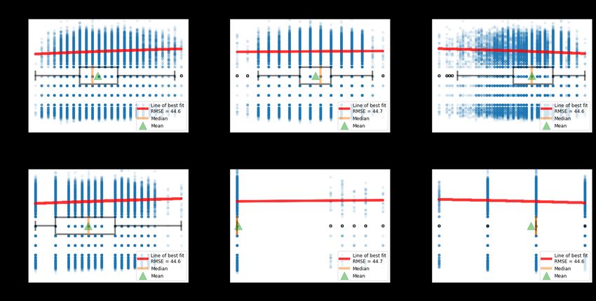
Event
Horizon
            Wheels-on          Gate-in         Gate-out     Wheels-off
              Time              Time            Time          Time

                 Observation             Predicting Departure                           Time
                  Window                    Gap      Delay
                                                                                  Schedule
                                                                         In air
                                                                                  Trajectory
      Start Gathering           Prediction                 Actual                 Actual
                                                                         Runway
         Features                 Time                    Gate-out                Trajectory
                                                                         Gate

Figure 1: An illustration of flight delay. We predict the departure delay which is between
the real gate-out time and scheduled gate-out time using the data extracted from observation
window.

representation [7, 6], and machine learning models [8, 9]. However, the problem
of departure delay is under-studied and more complex, as it is influenced by the
environmental factors, air traffic and also on-ground airport situations.
    Aerospace expert researchers have proposed a concept called air traffic com-
plexity (ATC) to describe airport traffic [10]. However, most works rely on es-
tablished equations based on empirical observations without offering any quan-
tification of the concept. In this context, Internet of Thing (IoT) -related tech-
niques such as sensor networks and big data analytics have the potential to
provide a scalable solution. Increasing works are exploring sensor networks in
the air traffic area [11, 12, 13]. They either use the sensor data to estimate the
traffic at the airport or monitor meteorological parameters.
    In this work, we address whether it is possible to predict the flight depar-
ture delay using big data from sensor networks, harnessing machine learning
and aerospace domain knowledge. Firstly, we represent the ATC using airport

                                                   3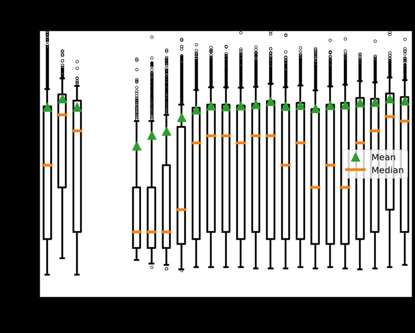
situational awareness maps (the trajectory of flights and vehicles at the air-
port). This work bridges the gap between the ATC – a concept proposed by
aerospace experts, sensor data fusion, and machine learning techniques. We ap-
ply two ways to represent the ATC: 1) we propose a group of features which are
extracted from sensor and radar data of aircraft at the airport, and 2) regard
the whole airport as a grid map and take a snapshot of each time period. The
locations, speed and other contextual information are represented as a sequence
of images. Secondly, we applied the factor analysis to both environmental data
and ATC data to explore the correlation between flight departure delay and
situational awareness map (ATC, weather, etc.). Thirdly, both of traditional
machine learning methods and a deep learning framework are used to predict the
flight departure delay with a real-world dataset of the Los Angeles International
Airport (LAX).
   The experimental results show that both the features we proposed to rep-
resent the ATC and the sequence of images we used to represent the airport
situational awareness map can be used to predict the flight departure delay,
and they are more effective than weather conditions and schedules. Addition-
ally, our proposed end-to-end deep learning framework also can predict the flight
departure delay with the comparable performance with machine learning-based
methods. We show that both the hand-crafted features based methods and the
end-to-end deep learning approaches can achieve similar results.
   The main contributions of this paper are the following:

   • We propose a generic framework to predict the departure delay using sit-
     uational awareness maps, original flight schedules and weather conditions.

   • We borrow a concept from aerospace area called Air Traffic Complexity
     (ATC), and use both aircraft trajectories and a sequence of snapshot of
     airport aircraft to represent this concept. We also analyse the importance
     of those features and compare them against previous delay-causing factors
     such as weather conditions and schedules.

   • We propose an approach to project the situational awareness map to a

                                       4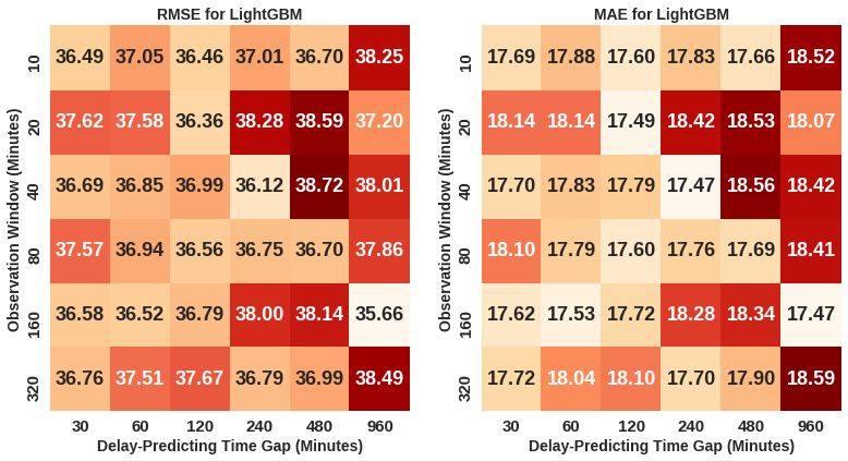
sequence of images and propose an end-to-end deep learning framework
     to predict the departure delay. The experimental results demonstrate the
     effectiveness of the approach to achieve a good result (less than 20 minutes
     prediction error).

   The paper is organised as follows: Section 2 discusses the related work; our
proposed methods are shown in Section 5; Section 6 shows the experiments
results; Section 7 discuss the current and future work, and Section 8 concludes
the paper.

2. Related Work

   There exists a large number of studies in the field of air traffic complex-
ity (ATC). However, the literature review shows that the majority of them are
considering using the complexity factors to indicate the currently existing or
expected impact on air traffic controller’s workload. Additionally, various stud-
ies on aircraft trajectory sensor data have shown to be effective in mobility
forecasting and map creation [14, 15].
   A polynomial equation was proposed by [10] which described ATC as the
combination of static sector characteristics and dynamic traffic patterns. An-
other metric approach called Dynamic Density (DD) was proposed as a measure
of ATC by NASA [16] and quickly became a well-known metric. The DD metric
is defined as a linear combination of multiple weighted traffic complexity factors
(TC); traffic density (TD) and air traffic controller intent (CI).
   A study proposed by NASA in 2007 [17] shows that the performance of the
complexity metrics varies at different facilities and conduct a further validation
on the 52 complexity variables for the Cleveland Centre. The paper by [18] lists
of all complexity factors proposed by the predecessors is given and an attempt
to reduce the size of that factor set is presented. The focus of the research by
[19] is to find a non-linear dynamical model which can differentiate the level of
the air traffic complexity based on vectorised aircraft locations.

                                         5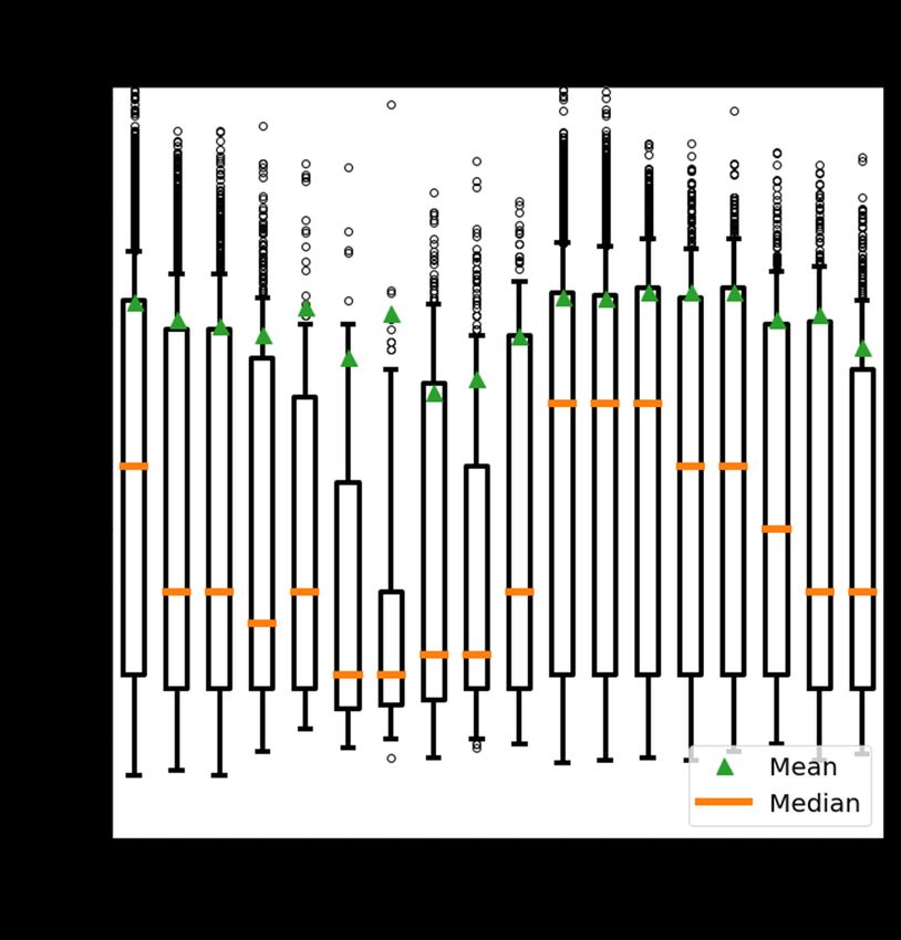
Since the researches mentioned above are mainly focused on the relationship
between ATC and air traffic controller workload, which normally exists in the
en-route environment. The research about airfield and airport traffic complexity
has received very little attention ([20], [21]), while the relationship between the
air traffic complexity and the gate-hold delay has had even fewer attention [6].
The study by [20] has a primary focus on the ATC around the tower area and its
influence on the air traffic controllers’ workload. It also shows that the relative
effectiveness of complexity metrics is site-specific due to the different layouts
and configurations of every airport. [21] proposed a new metric called Dynamic
Complexity which contains the features about the layout of a certain airport
and the traffic interactions in the airport itself and its vicinity.
   When considering predicting the departure delay of flights, the air traffic
complexity can be seen as one of the most important parts, since it connects
and captures the characteristics of several problems: the arrival delay prop-
agation problem, the runway sequencing problem. In [22], a snapshot of the
current departure delay state is used to characterise the current network state.
This snapshot is a 584-dimensional vector which comprises the current depar-
ture delay state of each link in a simplified US airport network and the delay
predictions at time t are made based on the snapshot at time t. The main fo-
cus of [23] is to classify the major factors that could cause or absorb the flight
delay. [6] discussed the seasonal weather trend the arrival flight delay propa-
gation effect but neglected factors that may describe the air traffic complexity.
In [6], departure delay is measured by the discrepancy between the scheduled
departure time and the actual departure time from the gate.

3. Definitions

3.1. Reference

   In what follows, we define a single flight, f = (fx , fy ), as a pair of vectors.
The vectors, fx and fy , represent the feature and label vectors respectively. Both
vectors contain ordered pairs of attributes and values associated with a single

                                          6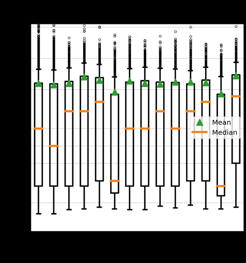
flight. All flights, f , are contained in the set, F. Furthermore, all flight features,
fx , and labels, fy , belong to their respective sets, Fx and Fy . The attributes of
a feature vector are listed in Table 1 and Table 2. This is also referred as the
reference data source.
   Meanwhile, the attributes of a label vector are:

   1. Delay Carrier (departure)
   2. Delay Weather (departure)
   3. Delay National Aviation System (departure)
   4. Delay Security (departure)
   5. Delay Late Aircraft Departure (departure)
   6. Departure Delay

   The Departure Delay is the sum of the total of all the other five types of
delays. Therefore, the performance metric is only based on the Departure Delay
attribute. The remaining attributes are used for labels to help with training.

3.2. ATC Features

   We define a GPS point, p ∈ P, as a vector of ordered pairs of attributes and
values. The attributes are:

   1. latitude
   2. longitude
   3. time
   4. speed
   5. heading

   There are also other attributes such as altitude and aircraft type, but we
removed these attributes during the data pre-processing step 5.1. These GPS
points are the basis for engineered features to capture Air Traffic Complexity
(ATC) as done in [24]. In this paper, we propose a novel set of ATC features
called TrajCNN Features based on these GPS points, described in Section 5.3.

                                          7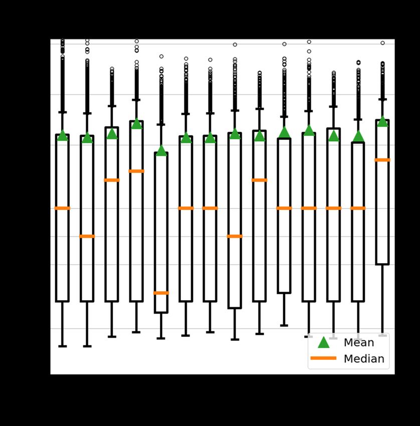
Table 1: The attributes feature vectors in the reference data source.

Attribute Name                 Description
                               The scheduled time when the aircraft
Scheduled departure
                               would depart from the gate. Also known
time
                               as gate-out time.
                               The scheduled duration when the aircraft
Scheduled elapsed
                               is on the air, between the current airport
time (departure)
                               (LAX), and the destination airport.
                               The scheduled time when the aircraft
Scheduled arrival
                               would arrive at the gate. Also known as
time
                               scheduled gate-in time.
                               The actual time when the aircraft arrived
Actual arrival time            at the gate. Also known as actual
                               gate-in time.
                               The scheduled duration when the aircraft
Scheduled elapsed
                               is on the air, between the origin and the
time (arrival)
                               current airport (LAX).
                               The actual duration when the aircraft
Actual elapsed time
                               was on the air, between the origin and the
(arrival)
                               current airport (LAX).
                               The actual time when aircraft wheel
Wheel on Time
                               touched the runway.
Delay carrier (arrival)        One of the five component of arrival delay.
Delay weather (arrival)        One of the five component of arrival delay.
Delay national aviation
                               One of the five component of arrival delay.
system (arrival)
Delay security (arrival)       One of the five component of arrival delay.
Delay late aircraft
                               One of the five component of arrival delay.
(arrival)
Arrival delay                  The total arrival delay.

                                        8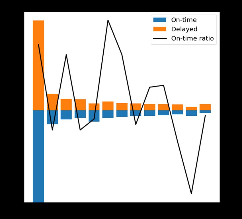
3.3. Problem definition

   Most airlines only have real-time details about their flights, but not flights
from other airlines. For this reason, to predict the Departure Delay, we will
only use features from the flight in question, fx , and not from any other flights.
However, to capture the spatio-temporal information on the airport tarmac,
airports could produce real-time aggregated and de-identified information with
posing significant privacy or security risk. We call these kinds of information as
ATC, defined in the previous subsection.
   Two factors affect the decision of when to make the prediction. On the one
hand, the prediction should be made as late as possible in order to capture the
most recent and relevant information. On the other hand, the earlier the predic-
tion, the more useful it will be for the airlines and the passengers. For example,
earlier delay predictions would allow passengers to adjust their schedules, while
late delay predictions might not allow for passengers to make any adjustment,
and thus, rendering the prediction obsolete. We decided that a realistic pre-
dicting gap is four hours as passengers are expected to arrive at the airport 3
hours before departure, giving appropriate time for passengers to adjust their
schedule before they arrive at the airports. We call this duration predicting gap.
   Our model will capture all the tarmac spatio-temporal information within
an observation window by creating a subset of P, called P0 . In turn, the ATC
features are constructed from P0 . Figure 1 illustrates predicting the time, ob-
servation window and the definition of departure delay, with is the difference
between the scheduled and actual departure (gate-out) time.
   Formally, for every flight, f ∈ F, we predict the Departure Delay, fy , using
only features about that particular flight, fx , and ATC constructed from a subset
of GPS points, P0 .

                                        9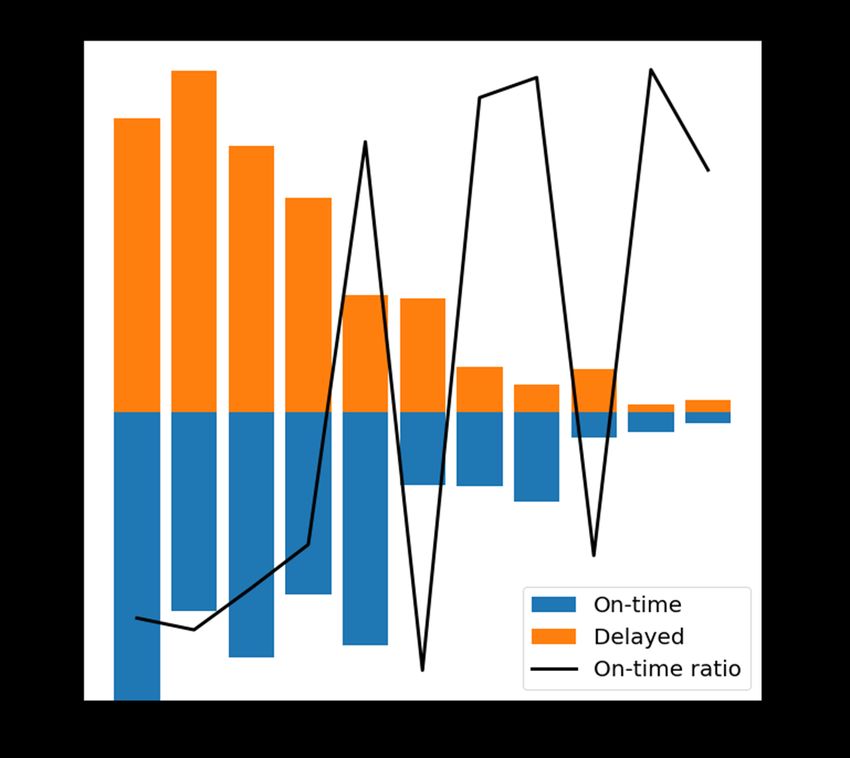
(a) Detailed statistics of historical flight delay   (b) Impact of Day of Week to flight delay.
in our dataset.

    (c) Impact of Tine of Day to flight delay. There were no flights between 3 and 5 AM.

 Figure 2: Detailed statistics of historical flight delay and the impact of temporal features.

                                               10
4. Dataset Analysis
4.1. Flight Delay
Figure 2(a) shows the detailed statistics of the flight delay in our dataset.
Note that departure delay exist for all flights, not just the ones delayed. Also,
departure delay can take negative value, meaning that the aircraft depart from
the gate early. Using very strict definition of on-time: departure delay ≤ 0, only
a little bit less than half of the flights are on time (49.4%) while the remaining
are delayed by at least one minutes. This is consistent with the median of the
delay being 1 minutes. However, this data is very skewed, as flights are unlikely
to leave very early, yet very long delay is more likely, thus the mean of the delay
(even including early departures) is 16 minutes, far higher than the median. The
problem of flight delay prediction is made difficult not by the average magnitude
of the delay, but by the high variability, measured by the standard deviation of
44.7 minutes.
It might be the case that these delay might easily be explained by a few
factors. However, in the remaining of this section, we will show that flight
delay prediction is a complex problem as it is not easily explained by any of the
features alone. Simple combinations of the features are explored in subsection
6.3.
The explainability of a feature is calculated through RMSE. The RMSE is
calculated by taking the average of each class and using it as the prediction.
Note that if we consider the entire dataset as one single class, then the RMSE
is equal to the standard deviation by definition. For this reason we use RMSE
as comparison of delay factor between different features.
Note that we do not use the airlines and airports information as features in
any of our models. The information are only provided here for completeness.
The full list of features are available in Table 1 and Table 2.
4.2. Day of Week and Time of Day
The first features we are going to analyse are the temporal features: Day
of Week (Figure 2(b)) and Time of Day (Figure 2(c)). Although the mean and
11median delay fluctuates throughout the week, the standard deviations remained
high. Taking the Day of Week effects into account, RMSE only goes down 0.05
from the standard deviation, showing that the Day of Week effect is small.
There is a stronger Time of Day effect compared to Day of Week effect. In
the morning before 10 AM, when the airport is more quiet, there are much less
delays. Nevertheless, the standard deviation within each hour is still very high.
Although the RMSE from Time of Day is smaller than Day of Week, it is still
only 1.1 minutes lower than the standard deviation.
4.3. Airlines and Airports
Next, we look at the effects of airlines, origin, and destination airports as
shown in Figure 3. The common theme is that although some airlines and some
airports has more delays than others, the variance within each group is still big,
with the lowest being destination airport with RMSE of 43.4.
As there are 77 origin and destination airports, we only pick the top 12 as
a part of our visualisation, and group the remaining into others. We pick the
number 12 as the combinations of these 12 airports represent more than 50% of
all the flights.
4.4. Weather
Finally, we analyse the relationship between many component of weather
with flight delay in Figure 4. For numerical variables, we draw the line of best fit
and calculate the RMSE from those. The weather condition of most flight is fair,
as expected from Californian cities. However, there are still sufficient variability
in weather conditions, temperature, humidity, and wind speed. Contrary to
expectation, fair weather has the lowest on-time ratio. This can be explained by
the fact that the standard deviation of delay during fair weather is higher than
the dataset (45.2 vs 44.7). This again suggested fair weather is not a significant
factor regarding delay. As also expected from most places, the geography of
a city is a huge determinant of wind direction, and thus we see that the wind
direction as clustered around Westerly winds.
12(a) (b)
(c) (d)
(e) (f)
Figure 3: The effect of airline and airport on departure delay.
13(a)
(b) (c)
(d) (e)
Figure 4: The effect of weather on departure delay.
14In this section, we conclude that temporal, airlines, airports, and weather
factors alone cannot satisfactory explain the huge variability in airport delay.
This suggests that we might need more information, such as spatial information
from within the airport, or that there are complex interplay of features that
necessitate the use of more powerful learners for flight delay prediction.
5. Methodology
The architecture of the flight departure delay time prediction system will be
described in this section. As shown in Figure 5, multiple datasets are gathered
including: the GPS sensor data of aircraft and vehicles in the tarmac area; the
historical flight data from major airline companies; and the associated weather
data. Besides the noise found, some datasets had redundant portions, and some
were incomplete. Therefore, a proper pre-processing procedure is required. To
this end, we apply the methods mentioned in [13] to make the datasets ready for
the next stage. More specific details will be discussed in the following section
5.1.
In the feature extraction stage, various methods were used to extract features
from the cleaned datasets. First, a partition of the whole ground surface of LAX
is used to separate different areas apart. Trajectories and GPS dots are counted
to represent the traffic density of those areas to form the baseline ATC, whereas
a more granular 2D histogram method was used to construct TrajCNN Features.
A principal component analysis (PCA) is used to reduce the dimensionality of
the weather data for the non-deep learning methods. The deep learning methods
could extract latent features directly from the raw data. We also extracted
multiple features from the combination of the historical flight scheduling data
and trajectory sensor data.
5.1. Data Pre-processing
As mentioned in the previous section, some datasets contain irrelevant and
redundant data. For example, the raw trajectory sensor data comprises the GPS
15Raw Flight Raw GPS Raw Weather
Schedule Record Data
Record
Data Cleaning One-hot Encoding
Arrival/Departure
Restore Trajectory PCA
Flight Matching
TrajCNN
Feature
Flight Reference
ATC Feature Weather Feature
Feature
Feature During
Observation Window
Flight Delay Experimental
Ground Truth Data
Figure 5: The demonstration of the overall system architecture.
(a) Three types of Tarmac area (b) Heatmap of the aircraft position
Figure 6: The tarmac area is classified into 3 types: apron/runway/parking area.
16records for ground vehicles, aircraft, and the historical flight scheduling data
contains ICAO (International Civil Aviation Organization) number. Besides
filtering out the irrelevant data points, it is also required to restore a continuous
trajectory of each flight based on the noisy data, which includes some random
jitter that falls within some impossible area. Therefore, we developed a data
pipeline that can ignore these random jitters. We also calculated the average
speed of the aircraft using the distance delta between two GPS records and
eliminated the outliers. After that, the pipeline could form a trajectory of each
flight based on its call sign and date since the same call sign is shared by all the
flights travelling on the same route. At the end of this stage, each trajectory will
be labelled into three different types based on which tarmac area the trajectory
encountered. An illustration of the three tarmac types: parking area, apron
area, and runway area are shown in Figure 6. Here the parking area indicates
that most aircraft move slowly in this area. Indeed, we checked the map of the
airport and found this area is for cargo purpose.
5.2. Feature Extraction
The features we used in this study can be classified into three categories:
Weather Features, ATC features and TrajCNN Features. The first two are
defined in Section 3; more details about the extraction of TrajCNN Feature are
described in the following section.
We matched every departure flight in LAX airport with their corresponding
arrival flight record in the historical scheduling table data. That will help to
introduce the possible delay propagation effect into consideration since the delay
of the current flight might not just come from the current situation, but also
has some relationship with the status of its previous arrival flight.
For the ATC data, we extracted features for each flight during its observation
window. As shown in Figure 1, the observation window is a duration period
before the prediction time. We extracted features from the ATC data listed in
Table 3. These features comprise a representation of the traffic density across all
17three aforementioned tarmac area areas. The number of potential landing/take-
off aircraft is also calculated to help reveal the complexity.
Table 2: The referenced weather features used in the feature vectors.
Attribute Name Description Type
Temperature The actual temperature at LAX (Fahrenheit). Real value
Dew point The temperature of dew point. Real value
Humidity Humidity at that time (%). Real value
Wind direction Wind Direction represented by string (e.g. SE). Categorical
The speed of the wind in that certain direction
Wind speed Real value
(mph).
Wind gust The potential increase in the speed of the wind. Real value
Pressure The ambient air pressure at LAX. Real value
Describing the state of the atmosphere in terms
Condition of temperature and wind and clouds and Categorical
precipitation (e.g. Cloudy).
For the non-deep learning methods, we performed a principal component
analysis (PCA) on the weather data to reduce the dimensionality. The PCA is
a statistical procedure which can reduce the dimension of a feature set while
still retaining most of the knowledge in it by transferring them into another set
of variables that are linearly uncorrelated [25]. After this process, the weather
data in Table 2 manages to get 18 principal components while still containing
its information. Furthermore, we use the most recent weather data within or
near the observation window for each flight.
Graph embedding is widely used in deep learning models especially for tra-
jectory data [26, 27]. However, for our model, we use the raw data because we
compared the results between using raw data and the graph embedding results
and found the raw data is a better option. It is because it is difficult for extract
accurate graph network from airport.
We converted the Wind Direction attribute, which was initially a categor-
18ical attribute (e.g. N/S/W/E/NW, etc.), to bearings in radians. We have
applied multiple machine learning approach to estimate the departure delay
with different data. We found that weather data, in most experiments, shows
no contributions to the prediction accuracy. Therefore, we did not consider it
in our deep learning model.
Table 3: The ATC feature description
Attribute Name Description
The number of aircrafts planning to take-off
takeoff plan
in the Delay-Prediction Time Gap.
The number of aircrafts that actually take-off
takeoff num
during the Observation Window.
The number of aircrafts planing to land in the
landing plan
Delay-Prediction Time Gap.
The number of aircrafts that actually land
landing num
during the Observation Window.
The discrete aircraft-GPS point count in the
apron point
apron area.
The discrete aircraft-GPS point count in the
runway point
runway area.
The discrete aircraft-GPS point count in the
patrol point
patrolling area.
The discrete aircraft-trajectory count in the
apron traj
apron area.
The discrete aircraft-trajectory count in the
runway traj
runway area.
The discrete aircraft-trajectory count in the
patrol traj
patrolling area.
195.3. TrajCNN Features
After we preprocess the GPS dataset, we then used these to construct Tra-
jCNN features to capture the spatio-temporal information from the airport tar-
mac for our deep learning model. For every flight, f , we first selected a subset of
GPS points that is within the flight’s observation window, P0 . Then, we divided
the airport into a 28 × 28 grid and perform three 2D histograms. We chose the
grid size of 28 as it is one of the common resolutions for CNN, such as MNIST.
The first channel is the counting channel while the subsequent two channels are
the of sum x- and y- velocity component on each grid, respectively. Then we use
a global scalar scaler to scale the pixel values between 0 and 1. We stack these
three channels into one image. This image is the TrajCNN features associated
with flight f .
5.4. SVR
Support Vector Machine (SVM) is a technique that was developed by Vladimir
Vapnik in 1995 [28]. It constructs a hyperplane in a high-dimensional feature
space. It was proposed to get a better result for classification problems. Later,
Drucker et al. [29] made some modifications to make it suitable for regression
tasks. This newer version is known as Support Vector Machine. The most cru-
cial step in this method is the production of the hyperplane. Exploiting kernel
methods to project the features into higher dimensional space could make the
classes linearly separable and improve results. There are two major factors in
this model: the parameter, ε, affects how close the fitting can be, and the pa-
rameter, C, controls model’s patience on the error. Changes in C causes the
degradation of the model’s generalisation ability.
5.5. MLP
The Multilayer Perceptron (MLP) is a feed-forward neural network, and its
structure is very self-explanatory. Each layer contains several units, and there
are one or more hidden layers that sit between the input and the output layer
[30]. An activation function can be applied to each node in this model, except the
20ones on the input layer. By introducing the activation function, the performance
on fitting non-linear relationships can be improved. In addition, increasing the
number of hidden layers can also help on the same goal, but might also cause
over-fitting. In our experiments, the MLP model has two hidden layers.
5.6. LightGBM
Gradient Boosting Decision Tree (GBDT) is a popular machine learning al-
gorithm in recent years, and it is an effective way of building a predictive model.
The basic idea is to generate multiple weak learners and use an additive model
on those weak learners to minimise the objective function, which is typically
formed as a loss function. In this paper, we use a newer variant of it, Light-
GBM, which was recently developed by Microsoft [31] as the GBDT framework
for the experiment. Although there are other implementations such as XGBoost
and pGBRT, the reason why we choose LightGBM is due to its several improved
features:
• The usage of histogram-based algorithms suppress the need of going through
all discrete values. That ends up in faster training speed and lower mem-
ory consumption.
• The implementation some advanced network communication algorithms
to utilise the multi-core processors for parallel learning.
As shown in Figure 7, the primary process in the LightGBM training is
to repeatedly create estimator, which is a weaker decision tree and test the
remaining loss based on all the weaker trees created so far.
Since departure delay prediction is a regression task, we use the Root Mean
Squared Error (RMSE) as the loss function.
5.7. TrajCNN
The Convolutional Neural Network (CNN) is one of the first architecture
in the now ubiquitous deep learning paradigm [32] [33]. It has been shown to
work well with image and image-like data [34] [35] [36]. As a result, many have
21Figure 7: The illustration of the LightGBM model creation process
GPS Point TrajCNN Features CNN
MLP
ATC
Latitude
Latent
… Features
Input Convolutional Pooling Output
Layer Layer Layer Layer
Longitude
Delay
.
Schedule Weather Schedule .
Time
.
Features
Weather .
.
Features .
Figure 8: TrajCNN architecture. We develop TrajCNN features to capture the spatiotemporal
information from the GPS points on the airport tarmac. We use CNN to map these features
into Air Traffic Complexity (ATC) latent features to represent the delay related complexity
of the airport. Then, we fuse this with the schedule information before feeding it to an MLP
regressor.
22attempted to engineer image-like features out of various problems [37]. This
includes spatio-temporal predictions such as traffic predictions [38] [39] [40].
Airport tarmac contains spatio-temporal information that would aid in solv-
ing the flight delay prediction problem [24]. Unlike the previous work that
divides the airport into tailored areas, we construct a novel TrajCNN feature
that would capture more information at a higher granularity as we make less
amounts of aggregation. The deep learning architecture would pick up latent
spatial-temporal features that might be lost during the coarse level aggregation
of the previous work.
The CNN architecture is as follows. The TrajCNN features are firstly fed into
two blocks of convolutional blocks. Each block consists of a convolutional layer,
a ReLu activation layer, and a 2 × 2 max-pooling layer, and the convolutional
layer has only one 3 × 3 filter. After flattening, it outputs the ATC latent
features that capture the delay related complexities of the airport. We fuse this
with the remaining flight features, fx ) and use it as an input to a fully connected
multilayer perceptron (MLP) with the delays fy as the output. The detail of
our architecture can be shown in Figure 8.
6. Experiment and Results
6.1. Datasets
In this section, we describe all data we used for our prediction in details.
6.1.1. Schedule Table Data
The first dataset consists of reference data operated by the Bureau of Trans-
portation Statistics of the United State Department of Transportation [41]. This
dataset is an open dataset, and we extracted the relevant parts from it which
comprise all flight records from the 1st of July, to the 31st of August. Both
arrival and departure flight information occurred in LAX are included since we
can extract features about the delay propagation effect from the former while
the latter provides the ground truth of the departure delay that we tried to pre-
dict. Except for the overall flight delay (both arrival and departure), the delay
23is partitioned and categorised into five different types for various causes. Addi-
tionally, it also contains the Call-sign/Tail-number, which helps us to match it
with our GPS trajectories data.
6.1.2. Weather Data
The second dataset in this experiment is reference data collected from web-
site [42]. This weather data mainly covers the Los Angeles Airport (LAX) and
some surrounding regions. It is gathered hourly, which provides a fine-grade
tracking of the weather condition. The essential numerical-based features are
temperature and humidity level. Meanwhile, the categorical features, Condition
and Wind Direction, are critical for later stages. We apply one-hot encoding on
the categorical features. More details are shown in Table 1.
6.1.3. Airport GPS Trajectories Sensor Data
The third reference dataset is a private dataset which consists of GPS ob-
servation of all vehicles and aircraft in the LAX (Los Angeles Airport). It
is collected by the United States’ Federal Aviation Administration’s (FAA’s)
System Wide Information Management (SWIM) program. Trajectories of all
vehicles can be restored based on this dataset. In the spatial domain, it covers
all the tarmac area of LAX while the vertical altitude goes up to 15000 metres.
In the temporal domain, the data contains seven weeks of data from the 1st of
July, 2016, to the 18th of August, 2016. There are around 11 million GPS points
fall within this range, which include both ground vehicles and aircraft locations.
We managed to restore 43,503 trajectories from it, which belongs 6,518 vehicles.
6.2. Experimental Setup
We withhold the last (28.6%, 2 weeks) of the dataset for testing, while we
use the remaining (71.4%, 5 weeks) for training and validation. We performed
cross-validation by dividing the dataset into 5 folds. The reason we chose this
method of cross-validation, instead of using the random split method, is because
each data point is temporally correlated with the other. We do this to ensure
no temporal correlation among each fold.
246.2.1. MLP
The hyper-parameter search space for MLP consist of:
• Number of nodes sampled from the following probability distribution:
N (x) = {nint(N × 2x )|x is distributed randomly over 2 ≤ x ≤ 12} where
N is a normalisation constant
• Number of layers sampled from the following probability distribution:
L(x) = {nint(R × x)|x is distributed randomly over 1 ≤ x ≤ 11} where L
is a normalisation constant
• Adam learning rate is sampled from the following probability distribution:
R(x) = {R × 2−x |x is distributed randomly over 9 ≤ 17 ≤ 2} where R is
a normalisation constant
Where nint(x) is a nearest integer rounding function.
6.2.2. LightGBM
The hyper-parameters for LightGBM in this experiment are shown in Ta-
ble 4, which also summarise the hyper-parameters for other models as well.
The three most important parameters are: learning rate, number of estimators,
and number of leaves. We also applied the early stop mechanism to avoid the
overfitting. All other parameters were left at their default settings. All hyper-
parameters are held unchanged through the whole testing procedure, which
includes a 5-fold cross-validation experiment and its following application on
the testing data-set.
6.2.3. TrajCNN
Since the training process for deep learning models is time-consuming, we
did not perform 5-fold validation. Instead, we randomly split the data with the
ratio of 7-1-2 for training-validation-testing, respectively. Our hyper-parameter
search space is as follows:
25• The number of fully connected layers is sampled from the following prob-
ability distribution: L(l) = {nint(L × l)|l is distributed randomly over
1 ≤ l ≤ 2} where L is a normalisation constant.
• The number of nodes in the fully connected layer is sampled from the
following probability distribution: N (n) = {nint(N × 2n )|n is distributed
randomly over 1 ≤ n ≤ 11} where N is a normalisation constant.
• The number of convolutional layers is sampled from the following prob-
ability distribution: C(c) = {nint(C × c)|c is distributed randomly over
1 ≤ c ≤ 4} where C is a normalisation constant.
• The number of filter in convolutional layer is sampled from the following
probability distribution: F(f ) = {nint(F × 2f )|f is distributed randomly
over 1 ≤ f ≤ 6} where F is a normalisation constant.
• The batch size is sampled from the following probability distribution:
B(b) = {nint(N × 2b )|b is distributed randomly over 1 ≤ b ≤ 8} where B
is a normalisation constant.
• The Learning rate is sampled from the following probability distribution:
R(r) = {N × 10−r |r is distributed randomly over 3 ≤ r ≤ 6} where R is
a normalisation constant.
We performed around 100 experiments and chose the hyper-parameter set
with the best validation RMSE. The best hyper-parameters can be found in
table 4. We then use this hyper-parameter set to train the final model on both
the training and validation dataset. Finally, we evaluate the final model on the
test dataset.
6.3. Experimental Results
In this section, we conducted three sets of experiments. In this first exper-
iment, we evaluated the prediction results using different combinations of data
sources and machine learning models. In the second experiment, we tested the
26Table 4: The Hyper-parameter using in this experiment
Hyper-parameter Attribute Name Value
Model SVR
Kernel type kernel rbf
The error term C 10000
Model MLP
Dropout is dropout False
Num of epoch n epoch 3000
Early stopping round n patience 50
Num of layers n layer 2
Num of node n node 1553
Adam learning rate adam learning rate 0.00976563
Model LigtGBM
Learning rate learning rate 0.01
Number of estimators n estimators 16000
Number of leaves num leaves 39
Model TrajCNN
Num of fully connected layer n fc layer 1
Num of node in fully connected layer n fc 429
Num of convolutional layer n conv layer 2
Num of filter in convolutional layer n conv 1
Batch Size batch size 15
Num of epoch n epoch 200
Early stop patience n early stop patience 20
Optimizer optimizer Adam
Learning rate adam lr 3.48981e-05
27temporal sensitivity of the learning model and validated the robustness of the
model in flight delay time prediction. In the last set of experiments, we com-
pared the importance of different features that we extracted and created from
the historical, ATC, and weather datasets. We conducted these three sets of
experiments to evaluate the performance of our proposed flight delay prediction
framework and the importance of our proposed ATC features.
In the first set of experiments, we apply four conventional machine learning
regressors: Linear Regression (LR), Support Vector Regressor (SVR), Multi-
layer Perceptron (MLP), LightGBM, and our proposed deep learning architec-
ture, TrajCNN, to predict the flight delay using different combination of data
sources (Historical, weather, and GPS data). In this experiment, we use the
traditional regression evaluation metrics: Root Mean Square Error (RMSE) to
measure the performance of flight delay time prediction using different models
and combinations of data sources. A Lower RMSE shows less error between
prediction value and ground truth.
As shown in Table 5, LightGBM has the best overall performance. We can
found out that there is a clear performance boost after adding spatiotemporal
information, either in the form of ATC features, or TrajCNN features. In fact,
without the spatiotemporal information, the RMSE of most algorithms is only
around the standard deviation of the label.
The best results come from the experiments that combines flight reference
data, ATC features, and weather data. These results indicate that the ATC
features play a significant role in predicting flight departure delay.
Linear Regression performs poorly no on linear features such as ATC fea-
tures, which other algorithms able to exploit well. Moreover, since we linearly
decorrelate the data using PCA, linear regression is received a minor boost in
improvement.
In the second set of experiments, we choose two temporal parameters to
validate the robustness of the prediction result. We use only LightGBM in this
experiment because it is one of the best performers with the shortest train-
ing time. The first parameter is the length of the observation window. As
28illustrated in Figure 1, the observation window is between the time point we
predict the flight delay and the time point we start to collect ATC and weather
data. The other parameter is the delay-predicting gap which starts from pre-
diction time and gate-out time (flight close the gate). From intuition, Longer
delay-predicting gap is likely to lead to worse results due to higher uncertainty.
Meanwhile, shorter observation window means less training data is used in the
model, which is likely to cause worse performance.
Figure 9: The RMSE and MAE flight departure delay prediction result by LightGBM using
the different observation window (x) and delay-prediction time gap (y) combinations.
In summary, prediction accuracy is stable with even less training data. Fur-
thermore, even the prediction time is four hours ahead of the flight delay event,
the accuracy (around 17 minutes) is acceptable.
In the third experiment, we compare the importance of features we used in
ATC dataset, weather condition dataset and historical dataset. We use the pa-
rameter f eature importance recorded by the LightGBM regressor, which cap-
tures the numbers of times a specific feature is used to ‘split’ a tree [43]. The
higher times this value is, the more information this feature provides, which
helps the model to differentiate the situation.
Figure 10 shows the feature importance after the training process. Firstly,
29Scheduled departure time 2948
* Num of aircraft actual land 1755
* GPS points in apron area 1732
* Num of aircraft plan to land 1681
* Num of aircraft plan to takeoff 1547
* GPS points in patrol area 1460
* Num of aircraft actual takeoff 1364
* Trajectories in patrol area 1131
weather feature_10 1030
weather feature_16 1004
weather feature_8 1002
* GPS points in runway area 973
weather feature_5 954
914
Importance
weather feature_12
* Trajectories in runway area 907
weather feature_14 887
weather feature_4 882
weather feature_1 864
weather feature_18 855
weather feature_17 813
Trajectories in apron area 793
weather feature_13 787
weather feature_2 730
weather feature_6 710
weather feature_3 687
weather feature_11 602
weather feature_15 579
weather feature_9 548
weather feature_7 424
0 500 1000 1500 2000 2500 3000
Feature Name
Figure 10: The feature importance for Weather and ATC features. All ATC features in this
graph has a red asterisk before them.
30Table 5: The RMSE result for different models and different combination of different data
sources. (* Not Applicable as TrajCNN have to use images from TrajCNN features to work.)
RMSE LR MLP SVR LightGBM TrajCNN
Flight Reference Only 44.3648 44.5027 44.3945 40.1237 *
Reference+Weather 44.3060 45.6198 44.0933 39.2137 *
Reference+ATC 44.3553 44.4964 43.9669 38.2711 *
Reference+Weather+ATC 44.3117 44.0964 43.896 37.9478 *
Reference+TrajCNN Features * * * * 37.2533
Reference+Weather
* * * * 38.6123
+TrajCNN Features
the historical data is still the most important feature (Schedule Departure Time)
in predicting departure delay. Secondly, we can find that most of our selected
ATC features have significantly higher importance than the weather features,
which also supports the result in the first experiment that the ATC features
does contribute more in this task.
7. Discussion and Future Work
Our proposed features and framework achieve an acceptable prediction per-
formance in flight departure delay problem. However, there remain many lim-
itations and potential work for the future. Firstly, this work mainly focuses
on predicting the departure delay using airport traffic data. We did not con-
sider many other traditional factors such as air traffic or airport traffic control
system. Secondly, due to the difficulty to collect data from airports, we only
chose the data from one airport, which limits the generalisation of our proposed
methods. Although our proposed solutions do not rely on any specific factor
of this airport, various data are still needed. Additionally, the seasonal pat-
tern also plays an important role in flight delay as well. However, due to the
range of the data provided by FAA, we only evaluate our system using a few
31months data. We plan to apply our proposed framework to different airports
in a longer time in future work. Thirdly, the proposed deep learning networks
can still be improved with more state-of-the-art techniques such as attention
mechanism and assign the temporal prediction ability to this network using re-
current components. Fourthly, due to the purpose of this paper is to estimate
the departure delay using only on-ground data at the airport, many factors such
as conditions of air route, destination, and airline (Hub or Non-Hub) are not
taken into account, which can also significantly affect the departure time. We
plan to incorporate these factors with on-ground GPS data to achieve higher
accuracy in the future. Additionally, many STOA CNN-based models have not
been applied to this data since the rapid development of the deep learning area.
Lastly, the existing work predicts the flight delay 4 hours before the scheduled
departure time based on the observation window. However, sometimes, people
or airport traffic controller needs a long horizontal prediction. We plan to apply
the existing model to various needs and long-term prediction in the future.
8. Conclusion
We have proposed to use airport traffic complexity (ATC) data combined
with traditional environmental factors to predict the flight departure delay from
heterogeneous sensor data. We have designed, implemented, and evaluated an
end-to-end deep learning-based framework to infer the delay time from a se-
quence of the snapshot of aircraft trajectories at the airport. We show in
our evaluation that our approach allows for estimating flight departure de-
lay with average deviations to the ground truth of fewer than 20 minutes.
http://www.cs.sjtu.edu.cn/ yaobin/ccf.htm Also, we have demonstrated that
the airport situational awareness map plays a more critical role in departure de-
lay time prediction than weather conditions, and analyse the correlation between
flight departure delay and ATC components. We also demonstrated that Light-
GBM outperforms other classic regressors using ATC feature, and a sequence
of the snapshot of aircraft can be used to represent the aircraft trajectories and
32predict the flight delay.
Acknowledgement
This research is funded by Northrop Grumman Corporations USA for ”Spatio-
temporal Analytics for Situation Awareness in Airport Operations” project,
RMIT University. We would like to also acknowledge the support of the CSIRO
Data61 Scholarship for Arian Prabowo and RMIT Research Stipend Scholarship
(RRSS) for Sichen Zhao. We also acknowledge the support of ARC Discovery
Project DP190101485.
References
[1] U.S. Government Accountability Office, Airline consumer protections addi-
tional actions could enhance dot’s compliance and education efforts, Tech.
rep., Department of Transportation (Nov 2018).
[2] U.S. Government Accountability Office, Airline passenger protections more
data and analysis needed to understand effects of flight delays, Tech. rep.,
Department of Transportation (Sep 2011).
[3] Y. J. Kim, S. Choi, S. Briceno, D. Mavris, A deep learning approach to
flight delay prediction, in: AIAA/IEEE Digital Avionics Systems Confer-
ence - Proceedings, Vol. 2016-December, 2016. doi:10.1109/DASC.2016.
7778092.
[4] A. Sternberg, J. Soares, D. Carvalho, E. Ogasawara, A Review on Flight
Delay PredictionarXiv:1703.06118.
URL http://arxiv.org/abs/1703.06118
[5] S. Ahmadbeygi, A. Cohn, M. Lapp, Decreasing airline delay propagation
by re-allocating scheduled slack, IIE transactions 42 (7) (2010) 478–489.
[6] Y. Tu, M. O. Ball, W. S. Jank, Estimating flight departure delay
distributions-a statistical approach with long-term trend and short-term
33pattern, Journal of the American Statistical Association 103 (481) (2008)
112–125.
[7] K. F. Abdelghany, S. S. Shah, S. Raina, A. F. Abdelghany, A model for
projecting flight delays during irregular operation conditions, Journal of
Air Transport Management 10 (6) (2004) 385–394.
[8] J. J. Rebollo de la Bandera, Characterization and prediction of air traffic
delays, Ph.D. thesis, Massachusetts Institute of Technology (2012).
[9] S. AhmadBeygi, A. Cohn, Y. Guan, P. Belobaba, Analysis of the potential
for delay propagation in passenger airline networks, Journal of air transport
management 14 (5) (2008) 221–236.
[10] R. H. Mogford, J. Guttman, S. Morrow, P. Kopardekar, The complexity
construct in air traffic control: A review and synthesis of the literature.,
Tech. rep., CTA INC MCKEE CITY NJ (1995).
[11] R. Trüb, D. Moser, M. Schäfer, R. Pinheiro, V. Lenders, Monitoring mete-
orological parameters with crowdsourced air traffic control data, in: Pro-
ceedings of the 17th ACM/IEEE International Conference on Information
Processing in Sensor Networks, IEEE Press, 2018, pp. 25–36.
[12] A. Prabowo, P. Koniusz, W. Shao, F. D. Salim, Coltrane: Convolutional
trajectory network for deep map inference, in: The 6th ACM International
Conference on Systems for Energy-Efficient Buildings, Cities, and Trans-
portation (BuildSys ’19), November 13–14, 2019, New York, NY, USA,
IEEE, 2019.
[13] W. Shao, F. D. Salim, J. Chan, K. Qin, J. Ma, B. Feest, Onlineairtrajclus:
An online aircraft trajectory clustering for tarmac situation awareness, in:
2019 IEEE International Conference on Pervasive Computing and Commu-
nications (PerCom, IEEE, 2019, pp. 192–201.
[14] G. A. Vouros, A. Vlachou, G. M. Santipantakis, C. Doulkeridis, N. Pelekis,
H. V. Georgiou, Y. Theodoridis, K. Patroumpas, E. Alevizos, A. Artikis,
34et al., Big data analytics for time critical mobility forecasting: Recent
progress and research challenges., in: EDBT, 2018, pp. 612–623.
[15] G. Andrienko, N. Andrienko, Creating maps of artificial spaces to explore
trajectories, in: Proceedings of the Workshop on Advanced Visual Inter-
faces AVI, ACM, 2018.
[16] I. V. Laudeman, S. Shelden, R. Branstrom, C. Brasil, Dynamic density:
An air traffic management metric, Tech. rep., NASA (1998).
[17] P. Kopardekar, A. Schwartz, S. Magyarits, J. Rhodes, Airspace com-
plexity measurement: An air traffic control simulation analysis, in: 7th
USA/Europe Air Traffic Management R&D Seminar, Barcelona, Spain,
2007.
[18] J. Djokic, B. Lorenz, H. Fricke, Air traffic control complexity as workload
driver, Transportation research part C: emerging technologies 18 (6) (2010)
930–936.
[19] D. Delahaye, S. Puechmorel, J. Hansman, J. Histon, Air traffic complexity
based on non linear dynamical systems, 2003.
[20] A. Koros, P. S. Rocco, G. Panjwani, V. Ingurgio, J.-F. D’Arcy, Complex-
ity in air traffic control towers: A field study. part 1. complexity fac-
tors, Tech. rep., FEDERAL AVIATION ADMINISTRATION TECHNI-
CAL CENTER ATLANTIC CITY NJ (2003).
[21] T. K. Simić, O. Babić, Airport traffic complexity and environment effi-
ciency metrics for evaluation of atm measures, Journal of Air Transport
Management 42 (2015) 260–271.
[22] J. J. Rebollo, H. Balakrishnan, Characterization and prediction of air traffic
delays, Transportation research part C: Emerging technologies 44 (2014)
231–241.
35[23] N. Xu, L. Sherry, K. Laskey, Multifactor model for predicting delays at us
airports, Transportation Research Record: Journal of the Transportation
Research Board 10 (2052) (2008) 62–71.
[24] W. Shao, A. Prabowo, S. Zhao, S. Tan, P. Koniusz, J. Chan, X. Hei,
B. Feest, F. D. Salim, Flight delay prediction using airport situational
awareness map, in: 27th ACM SIGSPATIAL International Conference on
Advances in Geographic Information Systems (SIGSPATIAL ’19), Novem-
ber 5–8, 2019, Chicago, IL, USA, IEEE, 2019.
[25] J. Li, R. R. Linear, Principal component analysis (2014).
[26] C. Chen, C. Liao, X. Xie, Y. Wang, J. Zhao, Trip2vec: a deep embed-
ding approach for clustering and profiling taxi trip purposes, Personal and
Ubiquitous Computing 23 (1) (2019) 53–66.
[27] X. Wang, C. Chen, Y. Min, J. He, B. Yang, Y. Zhang, Efficient metropoli-
tan traffic prediction based on graph recurrent neural network, arXiv
preprint arXiv:1811.00740.
[28] A. J. Smola, B. Schölkopf, A tutorial on support vector regression, Statistics
and computing 14 (3) (2004) 199–222.
[29] H. Drucker, C. J. Burges, L. Kaufman, A. J. Smola, V. Vapnik, Support
vector regression machines, in: Advances in neural information processing
systems, 1997, pp. 155–161.
[30] S. Haykin, Neural networks: a comprehensive foundation, Prentice Hall
PTR, 1994.
[31] G. Ke, Q. Meng, T. Finley, T. Wang, W. Chen, W. Ma, Q. Ye, T.-Y. Liu,
Lightgbm: A highly efficient gradient boosting decision tree, in: Advances
in Neural Information Processing Systems, 2017, pp. 3146–3154.
[32] Y. LeCun, B. Boser, J. S. Denker, D. Henderson, R. E. Howard, W. Hub-
bard, L. D. Jackel, Backpropagation applied to handwritten zip code recog-
nition, Neural computation 1 (4) (1989) 541–551.
36[33] Y. Le Cun, L. D. Jackel, B. Boser, J. S. Denker, H. P. Graf, I. Guyon,
D. Henderson, R. E. Howard, W. Hubbard, Handwritten digit recognition:
Applications of neural network chips and automatic learning, IEEE Com-
munications Magazine 27 (11) (1989) 41–46.
[34] K. Simonyan, A. Zisserman, Very deep convolutional networks for large-
scale image recognition, arXiv preprint arXiv:1409.1556.
[35] K. He, X. Zhang, S. Ren, J. Sun, Deep residual learning for image recog-
nition, in: Proceedings of the IEEE conference on computer vision and
pattern recognition, 2016, pp. 770–778.
[36] A. Krizhevsky, I. Sutskever, G. E. Hinton, Imagenet classification with
deep convolutional neural networks, in: Advances in neural information
processing systems, 2012, pp. 1097–1105.
[37] Y. Tas, P. Koniusz, Deep residual learning for image recognition, in:
BMCV, 2018.
[38] H. Yao, X. Tang, H. Wei, G. Zheng, Z. Li, Revisiting spatial-temporal
similarity: A deep learning framework for traffic prediction, in: AAAI
Conference on Artificial Intelligence, 2019.
[39] J. Wang, Q. Gu, J. Wu, G. Liu, Z. Xiong, Traffic speed prediction and
congestion source exploration: A deep learning method, in: 2016 IEEE
16th International Conference on Data Mining (ICDM), IEEE, 2016, pp.
499–508.
[40] X. Ma, Z. Dai, Z. He, J. Ma, Y. Wang, Y. Wang, Learning traffic as images:
a deep convolutional neural network for large-scale transportation network
speed prediction, Sensors 17 (4) (2017) 818.
[41] Weather-Underground, Los angeles international airport, california,
https://www.wunderground.com/history/daily/us/ca/los-angeles/
KLAX/date/2016-7-31/, [Online; accessed 5-Apr-2019].
37You can also read