Evaluation of the dual-polarization weather radar quantitative precipitation estimation using long-term datasets
←
→
Page content transcription
If your browser does not render page correctly, please read the page content below
Hydrol. Earth Syst. Sci., 25, 1245–1258, 2021
https://doi.org/10.5194/hess-25-1245-2021
© Author(s) 2021. This work is distributed under
the Creative Commons Attribution 4.0 License.

Evaluation of the dual-polarization weather radar quantitative
precipitation estimation using long-term datasets
Tanel Voormansik1,2 , Roberto Cremonini3,4 , Piia Post4,5 , and Dmitri Moisseev4,5
1 Institute of Physics, University of Tartu, Tartu, Estonia
2 Numerical   Modeling Department, Estonian Environment Agency, Tallinn, Estonia
3 Regional Agency for Environmental Protection of Piemonte, Department for Natural and Environmental Risks, Turin, Italy
4 Institute for Atmospheric and Earth System Research/Physics, University of Helsinki, Helsinki, Finland
5 Radar Science, Finnish Meteorological Institute, Helsinki, Finland

Correspondence: Tanel Voormansik (tanel.voormansik@ut.ee)

Received: 20 November 2019 – Discussion started: 10 January 2020
Revised: 3 December 2020 – Accepted: 2 February 2021 – Published: 12 March 2021

Abstract. Accurate, timely, and reliable precipitation obser-      threshold exhibited the best agreement with gauge values in
vations are mandatory for hydrological forecast and early          all accumulation periods. In both countries reflectivity-based
warning systems. In the case of convective precipitation, tra-     rainfall QPE underestimated and specific differential-phase-
ditional rain gauge networks often miss precipitation max-         based product overestimated gauge measurements.
ima, due to density limitations and the high spatial variability
of the rainfall field. Despite several limitations like attenu-
ation or partial beam blocking, the use of C-band weather
radar has become operational in most European weather              1   Introduction
services. Traditionally, weather-radar-based quantitative pre-
cipitation estimation (QPE) is derived from horizontal re-         Detailed surface rainfall information is of great importance
flectivity data. Nevertheless, dual-polarization weather radar     in many fields, not only for agricultural or hydrological ap-
can overcome several shortcomings of the conventional              plications. In the recent past the COST 717 Action entitled
horizontal-reflectivity-based estimation. As weather radar         “Use of radar observations in hydrological and NWP mod-
archives are growing, they are becoming increasingly im-           els” investigated the assimilation of weather-radar-based pre-
portant for climatological purposes in addition to operational     cipitation in numerical weather prediction (NWP; Macpher-
use. For the first time, the present study analyses one of the     son, 2004). Weather radar data have been assimilated in a
longest datasets from fully operational polarimetric C-band        variety of assimilation systems and models of increasing res-
weather radars; these are located in Estonia and Italy, in very    olution. At the beginning, latent heat nudging was the most
different climate conditions and environments. The length          popular technique (Gregorc̆ et al., 2000), while researchers
of the datasets used in the study is 5 years for both Esto-        have recently moved towards volume reflectivity assimilation
nia and Italy. The study focuses on long-term observations         techniques: for example, Schraff et al. (2016) proposed the
of summertime precipitation and their quantitative estima-         KENDA (ensemble Kalman filter for convective-scale data
tions by polarimetric observations. From such derived QPEs,        assimilation) operator to assimilate reflectivity volume data
accumulations for 1 h, 24 h, and 1-month durations are cal-        in the COSMO (COnsortium for Small-scale MOdelling)
culated and compared with reference rain gauges to quantify        model. For decades, gauge networks have provided the best
uncertainties and evaluate performances. Overall, the radar        reference datasets. The E-OBS 50-year daily European grid-
products showed similar results in Estonia and Italy when          ded interpolated dataset has been widely used in climato-
compared to each other. The product where radar reflectiv-         logical studies (Cornes et al., 2018). Gauge-based datasets
ity and specific differential phase were combined based on a       have well-known shortcomings in their low spatial resolu-
                                                                   tion and to a lesser degree temporal resolution. Precipitation

Published by Copernicus Publications on behalf of the European Geosciences Union.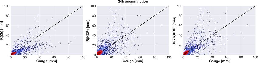
1246                   T. Voormansik et al.: Evaluation of the dual-polarization weather radar quantitative precipitation

data from satellites provide good spatial coverage but still        from the archive of weather radar scans set up for opera-
not in very high temporal resolution, especially in higher lat-     tional surveillance in the meteorological services. Secondly,
itudes (Sun et al., 2018). Polar-orbiting satellites provide bet-   the study areas are from heterogeneous climatologies, the
ter spatial resolution data in higher latitudes, but they are       weather radars being located in Estonia and Italy. This is
very limited in temporal resolution (Tapiador et al., 2018).        also the first ever study evaluating weather radar QPE in Es-
What is more, satellite-based precipitation estimates are lim-      tonia. What is more, we will assess the effect of the radar
ited by the accuracy of the estimates. The accuracy of the          scan interval as the radar data scan frequency is 5 and 15 min
estimates has a regional dependency and therefore can vary          from Italy and Estonia respectively. The study analyses result
due to the physiography of the study areas (e.g. precipitation      first in a few selected cases. The whole dataset is analysed at
climate, land use, and geomorphology) (Petropoulos and Is-          three accumulation intervals of 1 h, 24 h, and 1 month. Three
lam, 2017). Now that weather radars have already been used          radar QPE products are generated for comparison: first the
for decades in many countries, their archives are getting long      horizontal-reflectivity-based product R(ZH ), then the spe-
enough to use the data in climate studies (Saltikoff et al.,        cific differential-phase-based product R(KDP ), and as a third
2019). In the last decade, various studies have used multi-         radar QPE product, an R(ZH ) and R(KDP ) combination. To
year single-polarization weather radar data successfully in         investigate the performance of all these weather-radar-based
deriving rainfall climatology with high spatio-temporal res-        QPE products, they are compared with gauge accumulations.
olution (Overeem et al., 2009; Goudenhoofdt et al., 2016).             The paper is organized as follows. Section 2 describes the
However, quantitative precipitation estimation (QPE) with           rainfall estimation datasets from radar and rain gauges and
single-polarization C-band radar is strongly affected by at-        methods used for comparisons. The results are discussed in
tenuation of the electromagnetic wave in heavy precipitation        Sect. 3. In Sect. 4 conclusions are provided.
or a wet radome, hail contamination, partial beam blockage,
and absolute radar calibration (Krajewski et al., 2010; Cifelli
et al., 2011).
   All prior shortcomings can be mitigated by the use of
                                                                    2     Data and methods
dual-polarization weather radar data. Several studies have
shown that rainfall retrieved from dual-polarimetric radar
differential phase measurements outperforms rainfall esti-          2.1    Statistical methods for comparison
mated from horizontal reflectivity, especially in heavy pre-
cipitation (Wang and Chandrasekar, 2009; Vulpiani et al.,           To estimate the performance of the radar rainfall products,
2012; Wang et al., 2013; Crisologo et al., 2014). Because           they were compared with gauge accumulations. The study
differential phase measurements tend to be noisy and less re-       period was limited to the warm season (May–September
liable in low-intensity precipitation, Crisologo et al. (2014)      for Estonia and April–October for Italy). In Estonia, the
and Vulpiani and Baldini (2013) improved the robustness of          mean annual precipitation is 649 mm. Precipitation clima-
their rainfall retrieval technique by employing a combina-          tology has distinct seasonality, with a maximum in summer
tion of horizontal radar reflectivity R(ZH ) and specific dif-      (215 mm) followed by autumn (198 mm), winter (128 mm),
ferential phase R(KDP ), where a threshold was set below            and spring (108 mm). The summer maximum of seasonal
which R(ZH ) was used and above which R(KDP ) was used.             mean precipitation is especially pronounced in the continen-
Bringi et al. (2011) also compared performances of R(ZH ),          tal part of Estonia (246 mm in Mauri, south-east Estonia)
R(KDP ), and the combination product of the two on a rela-          (Tammets et al. 2013).
tively long set of data of 4 years.                                    In Piemonte, close to the radar, the mean annual precipi-
   The main aim of this study is to evaluate the potential of       tation is 870 mm having a bimodal distribution with peaks in
using polarimetric weather radar QPE on long-term warm-             spring (266 mm) and autumn (255 mm) (Devoli et al. 2018).
season datasets in various climatological environments. Pre-           Radar-based QPEs have been accumulated to the 1 h du-
vious studies in which the benefits of dual-polarimetric radar      ration, and longer durations have been calculated based
QPE have been shown are mostly based on selected short pe-          on these accumulations. Accumulations were calculated by
riods or only single events (Wang and Chandrasekar, 2010;           adding subsequent instantaneous radar QPE values without
Chang et al., 2016; Montopoli et al., 2017; Cao et al., 2018).      any space–time interpolation. No missing data for radar or
While the performance of the QPE methods can be com-                gauges were tolerated to prevent underestimation. A thresh-
pared based on short periods as well, only a study based            old of 0.1 mm was set and applied such that both gauge and
on long-term data can prove the robustness of a method and          radar QPE values must exceed this value to make the pair
suitability for long-term operational use. The uniqueness of        valid.
this paper is ensured by various features. First of all, we            The quality of the rainfall estimates was estimated by the
have a long 5-year dataset, starting already from 2011, de-         following verification measures (where ri is the ith out of n
rived by operational dual-polarimetric C-band weather radar         radar precipitation estimates, gi the ith out of n gauge ob-
made by different manufacturers. The dataset is gathered            servations, rm the mean of all n radar precipitation estimates,

Hydrol. Earth Syst. Sci., 25, 1245–1258, 2021                                        https://doi.org/10.5194/hess-25-1245-2021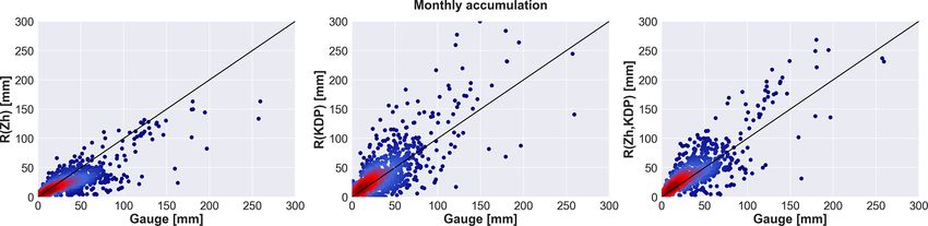
T. Voormansik et al.: Evaluation of the dual-polarization weather radar quantitative precipitation                          1247

and gm the mean of all n gauge observations).                     ated a regional automatic gauge network made up of about
                                                                  380 tipping-bucket gauges. Most of the gauges are heated to
Pearson’s correlation coefficient:
              Pn                                                  avoid solid precipitation accumulation during the cold sea-
                 i=1 (ri − rm ) · (gi − gm )                      son. The temporal resolution of the gauges network is 1 min.
 CC = qP                        qP                   .     (1)
            n
                (r  −  r   ) 2·     n
                                        (g   − g  )2              The Arpa Piemonte weather stations are equipped with CAE
            i=1   i      m          i=1    i    m
                                                                  PMB2 tipping-bucket rain gauges. Their resolution (0.2 mm)
Normalized mean absolute error:                                   is the amount of precipitation for one tip of the bucket. The
          Pn
                |ri − gi |                                        working range of measures is from 0 mm to 300 mm/h, with
 NMAE = i=1  Pn            .                               (2)    underestimation for high precipitation intensities. Such er-
               i=1 gi                                             rors are corrected according to results of the WMO Field In-
Normalized mean bias:                                             tercomparison of Rainfall Intensity Gauges (Vuerich et al.,
         Pn
              (ri − gi )                                          2009). An automatic data quality check is run on real-time
 NMB = i=1  Pn           .                                 (3)    data, followed by offline manned data validation. In this
              i=1 gi
                                                                  study, a network subset made of 42 rain gauges close to
Root mean squared error:                                          Turin, Italy, has been considered (Fig. 1). Precipitation mea-
         r
             1 Xn                                                 surements range from 2012 to 2016.
 RMSE =                (r − gi )2 .
                   i=1 i
                                                           (4)
             n
Nash–Sutcliffe efficiency:                                        2.3   Weather radar precipitation estimation
               Pn
                       (ri − gi )2                                Data from C-band dual-polarization Doppler weather radars
 NASH = 1 − Pni=1                 2
                                    .                      (5)
                  i=1 (gi − gm )                                  in Estonia and Italy were used in this study. The weather
The Nash coefficient is typically used to assess the accu-        radars considered in this study are from different manufac-
racy of hydrological predictions, but it has also been used for   turers, in Estonia Vaisala WRM200 and in Italy Leonardo
weather-radar-based rain rates and gauge comparisons (Nash        Germany GmbH METEOR 700C radar. Figure 1 illustrates
and Sutcliffe, 1970).                                             the location of the Estonian radar (Sürgavere) and the Ital-
                                                                  ian radar (Bric della Croce), together with the locations of
2.2   Rain gauge measurements                                     available rain gauges.
                                                                     Sürgavere radar, located in central Estonia at an altitude of
In Estonia major renewal and automation of the rain gauge         128 m a.s.l., has been operational since May 2008, but for
network run by the Estonian Environment Agency (EstEA)            this study data starting from 2011 were used because the
started in 2003. From 2003 to 2006 the network was up-            gauge network had been updated by that time. The radar per-
dated to automatic tipping-bucket gauges. Starting from 2006      forms a surveillance volume scan at eight elevation angles
the tipping-bucket gauges were progressively replaced by          (0.5, 1.5, 3.0, 5.0, 7.0, 9.0, 11.0, and 15.0◦ ) every 15 min,
weighted gauges. This process was finished by the end of the      starting each scan from the lowest elevation angle. Only the
year 2011. By that time there were 33 automatic weighted          lowest elevation angle data were used. The resolution of the
gauge stations and 27 stations with tipping-bucket gauges.        raw radar data is 300 m in range and 1◦ in azimuth. Data up
According to the comparative study of parallel measurements       to 10 km from radar were discarded because of the ground
of the tipping-bucket gauges and weighted gauges, the latter      clutter and unreliable KDP estimation. Close to the radar, sta-
exhibited much higher quality (Alber et al., 2015). From the      ble and reliable differential phase observations are not avail-
end of 2010, the data were recorded with a 10 min interval.       able due to both the antenna itself and the TR limiter’s re-
Until 2010 the temporal resolution was 1 h. Both 10 min and       sponse time or the dual-polarization switch in the case of
1 h data have been saved by EstEA since then, but only 1 h        alternate transmission. A Doppler filter was used to elim-
data have been quality-controlled by EstEA staff. Because         inate residual non-meteorological fixed clutter. In addition
the 10 min data are not quality-controlled, 1 h gauge data        to speckle and clutter-to-signal ratio filtering at the signal
were used in this study as a more reliable ground truth. The      processor level, polarimetric hydrometeor classification was
offline manned data quality control includes using mainly         used to filter non-meteorological targets from the display
weather sensor data as an additional source for comparisons       (Chandrasekar et al., 2013). After careful analysis, some of
but also neighbouring stations and weather radar data on          the data from Sürgavere radar had to be omitted completely.
some occasions. Only weighted gauge data were used be-            The years 2014 and 2015 were excluded because of gradu-
cause of the higher quality of these measurements and to          ally decreasing polarimetric data quality caused by a broken
ensure uniformness of the dataset. In this work, eight rain       limiter which was replaced in March 2016. Data from 2017
gauges close to Sürgavere, Estonia, are included (Fig. 1).        were discarded because the quality was inconsistent as a re-
Data have a resolution of 0.1 mm.                                 sult of a broken stable local oscillator (STALO), which was
   Since 1987, Arpa Piemonte, the Regional Agency for the         replaced in May 2018. From Estonia, the investigated period
Protection of the Environment, in Piemonte, Italy, has oper-      ranges then from 2011–2018 and includes 5 years of data.

https://doi.org/10.5194/hess-25-1245-2021                                      Hydrol. Earth Syst. Sci., 25, 1245–1258, 2021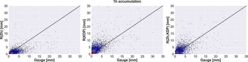
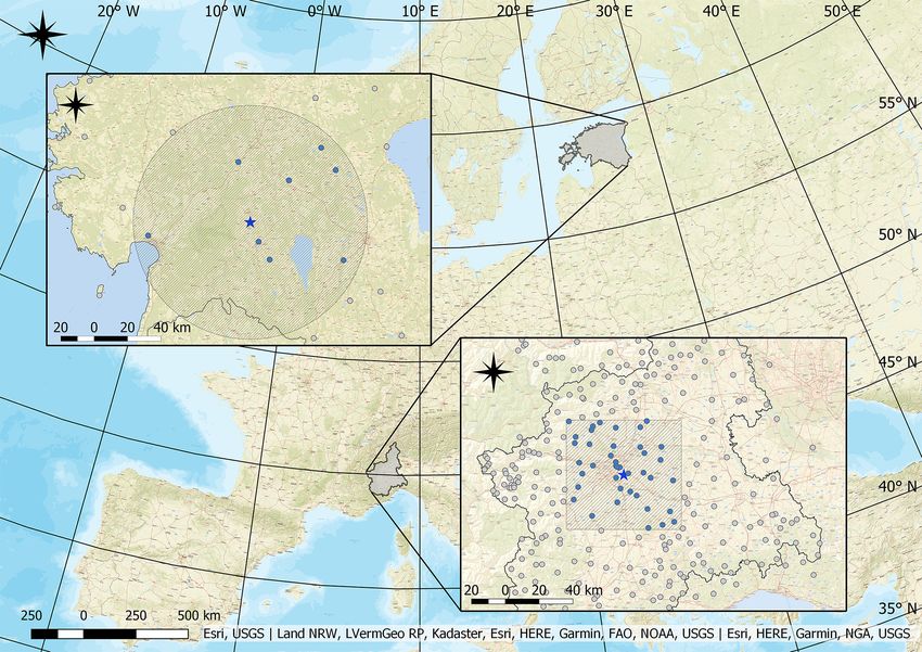
1248                    T. Voormansik et al.: Evaluation of the dual-polarization weather radar quantitative precipitation

Figure 1. Study areas (shaded) located in Estonia (upper left zoomed-in area) and in Piemonte, Italy (lower right zoomed-in area). Grey dots
denote gauge locations of both the Estonian and Piemonte region and blue dots gauges inside the study area. Blue stars reveal radar locations.

   On the Turin hill, at an altitude of 770 m a.s.l., the opera-         42 gauges respectively. By limiting data analysis to the warm
tional dual-polarization Doppler C-band weather radar Bric               season, and constraining the maximum radar range, we were
della Croce is located. The radar site is in the central part of         able to ensure that radar data were mainly originating from
the Piemonte region: toward west and north at about 20 km                liquid precipitation (hail can also occur), which is required
the Alps start, with peaks 2500–3000 m above sea level. The              for more reliable rainfall intensity estimation. The possible
radar performs fully polarimetric volume scans, made up of               occurrence of hail was not removed from the data because
11 elevations up to the 170 km range, with 340 m range bin               of the intention to keep additional data processing minimal
resolution. Bric della Croce observations used in the study              and to allow for equal comparison of the various QPE meth-
ranged from 2012 to 2016, whereas observations from 2012                 ods. In the case of Italy, the applied range limit is also aimed
to 2013 have a 10 min interval and from 2013 to 2016 have a              at eliminating uncertainties due to complex orography, like
5 min interval. As can be seen from Fig. 1, a circular area              shielding by the mountains, overshooting, and bright-band
around the radar is used in Estonia, but in Italy a rectan-              contamination.
gular area is used. The reason for this is that orography in                QPEs, based on horizontal reflectivity, are extensively de-
Piemonte is very complex, ranging from flat plains in the                scribed by Cremonini and Bechini (2010) and by Cremonini
Po valley (about 100 m a.s.l.) to the Alps up to more than               and Tiranti (2018); meanwhile, KDP precipitation estimates
4000 m a.s.l. The Bric della Croce weather radar is located              are derived according to Wang and Chandrasekar (2009).
on Turin hill, which is about 30 km from the Alps. Therefore,            When KDP was equal to or less than zero, then R(KDP ) was
the elegant and simple limitation in range by some kilometres            set to zero. The area close to the weather radar up to 8 km has
from the radar site does not work. To avoid mountainous ar-              been left out due to heavy ground clutter contamination and
eas, where there is partial and total beam blocking and where            unreliable estimations of KDP .
heavy ground contamination increases, a rectangle area, that                The Sürgavere radar specific differential phase product
extends towards flat grounds, has been preferred.                        (KDP ) and differential propagation phase product (ØDP ) were
   The maximum distance of the gauges to be included in                  recalculated from raw ØDP data using the Python ARM
the comparison was limited to a 70 km radius from the radar              Radar Toolkit (Py-ART) (Helmus and Collis, 2016) func-
location in the case of Estonia and up to 30 km distance in              tion phase_proc_lp (Giangrande et al., 2013), with carefully
Italy. Thus, in Estonia and Italy rainfall data were from 8 and          tuned parameter values according to data specifics. With de-

Hydrol. Earth Syst. Sci., 25, 1245–1258, 2021                                               https://doi.org/10.5194/hess-25-1245-2021
T. Voormansik et al.: Evaluation of the dual-polarization weather radar quantitative precipitation                           1249

fault parameter values, the rays where differential propaga-        verification measures introduced in Sect. 2.1 (Eqs. 1–5). The
tion phase folding occurred did not unfold correctly, and           verification results are presented in Table 1. The QPE product
thus the function did not produce correct specific differen-        based on recalibrated reflectivity (R(ZH cal )) shows clearly
tial phase values. To fix the folding issue, function parame-       superior results compared to the non-calibrated reflectivity-
ters self_const (self-consistency factor) and low_z (the low        based product (R(ZH def )), most notably by decreasing the
limit for reflectivity – reflectivity below this value is set to    negative bias.
this limit) had to be tuned. The self-consistency factor takes         To convert reflectivity ZH to rainfall rate R (mm/h), the
into account the spatial variability of reflectivity and differ-    following relation was used:
ential reflectivity within a given path. It is used to improve
                                                                    ZH = 300R 1.5 .                                            (6)
KDP field behaviours to more closely follow the cell patterns
found in ZH . The default values for self_const and low_z           Specific differential phase KDP was converted to rainfall rate
were 60000.0 and 10.0 respectively, and after testing with          using the expression suggested by Leinonen et al. (2012):
various combinations of various values the values 12000.0                    0.720
                                                                    R = 21.0KDP    .                                           (7)
and 0.0 were found to produce optimal results and there-
fore were chosen for final calculations. The values were first      The QPE of R(ZH ) can be affected by attenuation on C-
chosen after preliminary tests with single scans from mul-          band radars, especially in heavy precipitation and at long dis-
tiple years between 2011–2018 and then confirmed after a            tances. While this can be corrected using ØDP in our study,
final test with 1 month of 1 h accumulation data from August        it was not applied to the reflectivity data so as to not intro-
2018. The quality of the results was evaluated by using the         duce another possible source of error between the results of
verification measures introduced in Sect. 2.1 (Eqs. 1–5). The       Estonia and Italy that could not be easily quantified. The ef-
final test results are shown in Table 1. The product with opti-     fectiveness of attenuation correction using ØDP is hampered
mal values for the KDP processing algorithm (R(KDP tuned ))         by its temperature, shape, and size distribution dependence,
improves all verification measures when compared to the             which affect the accompanying error (Vulpiani et al., 2008).
product based on the KDP processing with default parame-            The QPE of R(ZH ) can also be affected by the effect of the
ter values (R(KDP def )). The KDP retrieval process involves        non-uniform vertical profile of reflectivity (VPR). In the cur-
filtering that reduces the range resolution of KDP to approx-       rent study, the effect of VPR will be limited because only
imately 1 km. Horizontal reflectivity (ZH ) was recalibrated        data from the warm season were used, and distance limits
using a method that utilizes the knowledge that ZH , ZDR (dif-      to the radar data were set (70 km for Estonia and 30 km for
ferential reflectivity), and KDP are self-consistent with one       Italy, respectively).
another and that one can be computed from two of the oth-              Several studies have shown that R(KDP ) provides much
ers. ZDR is not suitable for QPE on C-band radars, but it can       more reliable intensity estimates in heavy rainfall (Vulpi-
be used in this calibration methodology after applying strict       ani et al., 2012; Wang et al., 2013; Chen and Chandrasekar,
restrictions on the data used for this purpose. The calibration     2015). On the other hand, it has been indicated that KDP
was carried out using the self-consistency theory set down in       retrieval itself is less reliable in light precipitation condi-
Gorgucci et al. (1992, 1999) and Gourley et al. (2009), where       tions (Giangrande and Ryzhkov, 2008; Ryzhkov et al., 2014).
the methodology is described in detail. The method essen-           Thus, combining the two methods has the potential to be su-
tially compares the observed differential propagation phase         perior to using each method separately. For example, Vulpi-
product (ØobsDP ) to a calculated theoretical differential propa-   ani et al. (2013) used a weighted combination of R(ZH ) and
gation phase product (ØDP th). The data used for calibration        R(KDP ), where only reflectivity data were used for bins with
had to be filtered using several restrictions: only data from       KDP less than or equal to 0.5◦ /km, and KDP was used addi-
June to September were allowed; only data from 0.5◦ ele-            tionally with increasing weight above that value up to 1◦ /km,
vation and 10–70 km range were used; only bins where the            above which it was solely used. Cifelli et al. (2011) used
horizontal and vertical polarization channel correlation co-        a simple threshold method where R(KDP ) was used when
efficient was over 0.92 were used; any bins where ØDP was           R(ZH ) exceeded 50 mm/h intensity. Several authors have
greater than 12◦ were removed; whole rays where reflectiv-          successfully added R(ZDR )-based intensity estimation to the
ity was greater than 50 dBZ were removed; whole rays where          combination of S-band weather radars (e.g. Ryzhkov and Zr-
ZDR was greater than 3.5 dB were rejected; only rays where          nic, 1995; Ryzhkov et al., 2005; Chandrasekar and Cifelli,
1Øobs                         ◦
     DP was greater than 8 and where the consecutive rain           2012). Due to residual effects such as resonance, noise, and
path was at least 10 km were used; any scans in which precip-       attenuation, R(ZDR ) should not be used for C-band radars
itation occurred on top of the radome were removed. As a re-        (Ryzhkov and Zrnic, 2019).
sult, ZH bias values from the range of −2.0 to −5.0 dB were            In our study rainfall from a combined threshold ap-
obtained depending on the date. The bias values were used to        proach was used for both weather radars as a third product
correct the corresponding observed ZH before to rain rate es-       R(ZH , KDP ). In the combined product, R(ZH ) was used in
timation. The impact of the recalibration was evaluated on 1        areas with ZH less than or equal to 25 dBZ and R(KDP ) oth-
month of 1 h accumulation data from August 2018 using the           erwise if available. The ZH threshold value was selected after

https://doi.org/10.5194/hess-25-1245-2021                                        Hydrol. Earth Syst. Sci., 25, 1245–1258, 2021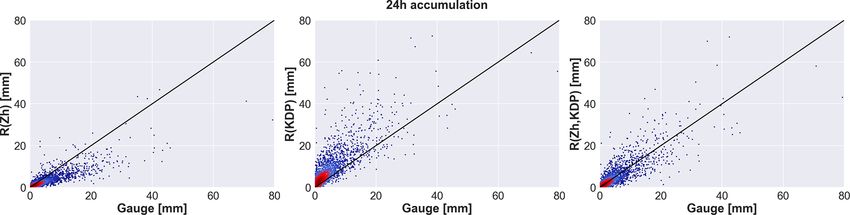
1250                   T. Voormansik et al.: Evaluation of the dual-polarization weather radar quantitative precipitation

Figure 2. The 1-month 1 h rainfall cumulative accumulations for      Figure 3. The 1-month 1 h rainfall cumulative accumulations for
Sürgavere radar data and Jõgeva station gauge data. ZH is not cor-   Sürgavere radar data and Tartu-Tõravere station gauge data. ZH is
rected for attenuation.                                              not corrected for attenuation.

                                                                     pensation is applied, QPE estimated by R(ZH ) shows lower
testing with various reflectivity levels. The reflectivity thresh-
                                                                     NMAE in Estonia. The difference in NMAE of R(KDP ) and
old was selected after verifying QPE performances at differ-
                                                                     R(ZH ) QPEs might stem from different precipitation regimes
ent reflectivity levels from 15 to 35 dBZ in 5 dBZ steps. The
                                                                     (more intense precipitation in Italy).
evaluation was based on 1 h accumulation rainfall for August
2018 in Estonia, and the verification statistics introduced in
Sect. 2.1 (Eqs. 1–5) were applied using the same gauges em-          3     Results and discussion
ployed in the latter parts of the study as reference. From Ta-
ble 1 it can be seen that the best scores are reached using          3.1    Case comparisons
25 dBZ (QPE product R(ZH25 , KDP )). The same evaluation
for the R(ZH , KDP ) algorithm was carried out for Bric della        In this section radar QPE products are compared with single-
Croce in Italy with a 1 h accumulation period, and it also con-      location gauge measurements of selected short periods from
firmed the suitability of the 25 dBZ level. The threshold level      Estonia and Italy. This allows for evaluating the performance
is considerably lower than some of the thresholds used in the        of the radar QPE against gauge measurements from a time-
literature referred to above, but on our datasets it performed       series viewpoint.
the best.                                                               Figure 2 shows 1 month of precipitation at the Jõgeva
   The impact of the temporal sampling was analysed using            station location (60 km away from the radar site) in Es-
Italian Bric della Croce weather radar second-elevation PPI          tonia with 1 h temporal resolution. Overall, radar products
(plan position indicator) data, which produce a 5 min inter-         follow the gauge measurements well, but there are consid-
val dataset. A degraded dataset of a length of 1 d, 10 Octo-         erable differences among them. Reflectivity-based product
ber 2020, with a 15 min sampling rate, was created by re-            R(ZH ) is not affected by noise and clutter in clear weather
moving two out of three files. Hourly accumulation was cal-          or light rain cases, but on the other hand, it underesti-
culated based on both sampling rates, which resulted in a            mates rainfall amounts particularly in medium- to heavy-
sample size of 253 514. As expected from the comparison of           precipitation cases. By the end of the month, its sum of
these accumulation pairs, the obtained normalized mean bias          40.5 mm was 19.6 mm less than gauge-measured accumu-
was close to zero (0.03), while the correlation coefficient was      lation (70.1 mm). R(KDP ) then again heavily overestimates
0.922, and the normalized mean absolute error was 0.21.              precipitation amounts, especially during light rain cases. By
   If we compare different skill scores for 1 h QPEs in Esto-        the end of the month, the accumulated amount of 150.2 mm
nia and Italy, part of the differences in correlation coefficient    was more than double the gauge sum. The third product,
and normalized mean absolute error can be explained as be-           R(ZH , KDP ), showed the best performance of all the three
ing due to different time sampling. Table 2 below summa-             compared, and it correlated well with gauge accumulation
rizes correlation coefficient and normalized mean absolute           time series; the 1-month accumulation of 69.5 mm was just
error values in Estonia and Italy.                                   0.6 mm lower than the rain gauge sum.
   Compensating the values obtained in Estonia for loss                 Gauge and radar accumulations are not always so well cor-
of correlation (0.078) and increased NMAE (0.21) due to              related as Fig. 3 demonstrates. In this accumulation period,
15 min time sampling with values estimated in Italy, it is vis-      there are rainfall events which show that gauge values can
ible that CC and NMAE are comparable in Estonia and Italy            be both under- and overestimated by radar products. Rainfall
(last row in Table 2). It is worth noting that after the com-        around 11 June 2016 is overestimated by all radar QPE prod-

Hydrol. Earth Syst. Sci., 25, 1245–1258, 2021                                         https://doi.org/10.5194/hess-25-1245-2021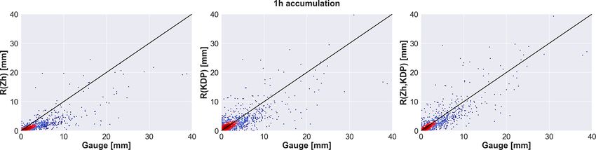
T. Voormansik et al.: Evaluation of the dual-polarization weather radar quantitative precipitation                                        1251

Table 1. Verification results of the test dataset of 1 month (August 2018) of the radar-based rainfall 1 h accumulation products of Estonia.
ZH is not corrected for attenuation.

                             R           R              R              R      R(ZH15 ,    R(ZH20 ,      R(ZH25 ,   R(ZH30 ,    R(ZH35 ,
                       (ZH cal )   (ZH def )   (KDP tuned )     (KDP def )      KDP )       KDP )         KDP )      KDP )       KDP )
       CC                0.699      0.699           0.659          0.428          0.687       0.721       0.726      0.713       0.705
       NMAE              0.572      0.634           1.074          1.491          0.855        0.69       0.605      0.596       0.595
       NMB              −0.212     −0.421           2.652          4.958          1.441       0.655       0.067     −0.118      −0.184
       RMSE (mm)         1.611      1.709           2.329          2.656          2.071       1.832       1.714      1.718       1.704
       NASH              0.247      0.202          −0.088         −0.241          0.032       0.144       0.199      0.197       0.204

Table 2. Verification of the 1 h accumulation QPE products of Estonia and Italy and differences without (“Difference”) and with (“Comp.
diff”) compensating for the impact of the temporal sampling. CC and NMAE values are obtained from Tables 3 and 4. ZH is not corrected
for attenuation.

                                         R          R         R (ZH ,                             R          R     R(ZH ,
                                       (ZH )     (KDP )        KDP )                            (ZH )     (KDP )    KDP )
                    CC (Estonia)      0.679      0.674         0.697    NMAE (Estonia)         0.537       0.868    0.594
                    CC (Italy)        0.843      0.808         0.870    NMAE (Italy)           0.531       0.514    0.423
                    Difference       −0.164     −0.134        −0.173    Difference             0.006       0.354    0.171
                    Comp. diff.      −0.086     −0.056        −0.095    Comp. diff.           −0.204       0.144   −0.039

ucts, with the smallest overestimation by R(ZH ) and greatest
by R(KDP ), which overestimated the gauge by more than 2
times in this event. In the following days until 21 June 2016,
light to medium precipitation was recorded by the gauge, and
during this time R(KDP ) mostly overestimated the gauge ac-
cumulations, while R(ZH ) underestimated rainfall. On the
21 June 2016, a convective rainfall event occurred during
which 51 mm of rainfall was measured in 2 h with a gauge.
All radar QPE products underestimated the rainfall amount
during this event. By the end of the month-long accumu-
lation period, R(ZH , KDP ) was closest to the gauge value
(underestimation by 16.6 mm), while R(ZH ) underestimated
even more, and R(KDP ) again overestimated gauge measure-
ments.                                                                       Figure 4. The 1 h rainfall cumulative accumulations from
   Figure 4 illustrates a case from Italy, a comparison of a                 Verolengo gauge, located 29 km from the radar, and co-located Bric
gauge located within 30 km distance from the radar to Bric                   della Croce radar QPE. ZH is not corrected for attenuation.
della Croce radar precipitation estimation products. At the
end of the 34 h period, the specific differential-phase-based
product R(KDP ) has the smallest error compared to gauge
as it overestimates the gauge measurement of 40.6 mm by                      pared to gauge data. At the end of the period, the accumu-
2.0 mm. On the other hand, in light rain R(KDP ) overesti-                   lated value for R(ZH , KDP ) was 26.7 mm.
mated significantly – in the first 13 h when a gauge mea-                       In all selected cases the general behaviour of QPEs is simi-
sured 3.4 mm of accumulated rainfall, it had already esti-                   lar. Weather radar estimations, even when sampled by 15 min
mated 12.2 mm. R(ZH ) underestimated, even in light rain,                    interval observations, follow gauge measurements with good
and in heavy rain, the difference compared to gauge mea-                     agreement, although the second case from Estonia illustrated
surement increased further. At the end of the period, the un-                well that a longer scan interval increases the scatter and par-
derestimation was nearly 3-fold (15.6 mm compared to gauge                   ticularly with small-scale convective precipitation, for which
accumulation of 40.6 mm). The R(ZH , KDP ) product showed                    a minimal sampling interval is the most beneficial. From
good correlation with gauge measurement in light precipita-                  Italy, the example case was much shorter, but the precipi-
tion as it was mostly based on reflectivity data, but in the case            tation intensity was higher. In both cases, R(KDP ) generally
of more intense precipitation, it still underestimated com-                  overestimates precipitation amounts, especially in light rain
                                                                             cases. In Italy, the R(KDP ) overestimation is smaller. One of

https://doi.org/10.5194/hess-25-1245-2021                                                 Hydrol. Earth Syst. Sci., 25, 1245–1258, 2021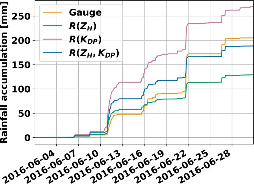
1252                   T. Voormansik et al.: Evaluation of the dual-polarization weather radar quantitative precipitation

Table 3. Verification of the radar-based rainfall 1 h accumulation      Table 3 presents the verification results for the hourly ac-
products of Estonia. ZH is not corrected for attenuation.            cumulation interval in Estonia. Figure 5 shows the corre-
                                                                     sponding scatter plots. As can be seen, the R(ZH ) estimation
                              R          R      R(ZH ,               generally underestimates rainfall, especially heavy events,
                            (ZH )     (KDP )     KDP )               while it has the best error verification values (Nash–Sutcliffe
           CC              0.679      0.674      0.697               efficiency 0.214, NMAE 0.537, NMB −0.143, and RMSE
           NMAE            0.537      0.868      0.594               1.615 mm). R(KDP ) on the other hand overestimates ac-
           NMB            −0.143      1.861      0.298               cumulations for low-intensity events as could be presumed.
           RMSE(mm)        1.615      2.131      1.677               R(ZH , KDP ) shows considerable improvement by combining
           NASH            0.214     −0.037      0.184               strong aspects of the two methods. It has the highest correla-
                                                                     tion coefficient (0.697) of all the products.
                                                                        Nevertheless, it can be seen from the scatter plots that there
Table 4. Verification of the radar-based rainfall 1 h accumulation   is a lot of scatter in the hourly radar accumulations with all
products of Italy. ZH is not corrected for attenuation.
                                                                     products. Mostly, it can be linked to the low spatial repre-
                                                                     sentativeness of the point measurements of rain gauges. This
                               R        R      R(ZH ,
                                                                     effect is more pronounced on a short timescale, and it orig-
                             (ZH )   (KDP )     KDP )
                                                                     inates from a scarce gauge network and insufficient radar
           CC               0.843     0.808     0.870                scan rate. Small-scale effects like wind drift might also be
           NMAE             0.531     0.514     0.423                more influential on a shorter accumulation period (Lauri et
           NMB             −0.296     0.678     0.120                al., 2012). The reason why R(ZH ) might have the best per-
           RMSE(mm)         3.136     3.037     2.750                formances when NMAE and RMSE are considered is that
           NASH             0.364     0.385     0.443
                                                                     there are not very many heavy rainfall cases in Estonia, and
                                                                     this tends to favour R(ZH ) in the verification comparisons.
                                                                        From Italian hourly accumulation scatter plots in Fig. 6,
the causes of this behaviour might be more intense precipi-          it can be seen that the overall behaviour of the radar prod-
tation in Italy for which KDP measurement was more accu-             ucts is similar to Estonia, although from Fig. 6 it can be no-
rate. More intense rainfall on the other hand caused greater         ticed that of the four highest 1 h accumulations measured by
underestimation of R(ZH )-based precipitation accumulation           the gauge, three of them have significantly higher radar es-
from gauge values compared to Estonia. Another cause of              timates for R(ZH , KDP ) than either R(ZH ) or R(KDP ). This
differences between the two countries might be differences           could be explained by precipitation that was very variable in
in the drop size distribution climatologies. Rainfall retrieval      intensity and also in spatial coverage in these three cases,
relations also cause errors, and to keep the comparison as           which in turn caused unsteady behaviour of the precipita-
uniform as possible, we decided to use the same relations for        tion estimates. ZH underestimates high intensities, but with
both Italy and Estonia. These example cases demonstrated             low intensities, KDP becomes noisy, and the rainfall inten-
that radar can be used for 1 h accumulations, but system-            sity estimation is not feasible. Finally, to reduce KDP uncer-
atic errors cannot be excluded. These cases also presented           tainties, range averaging is mandatory, leading to underesti-
the shortcomings of studies based only on a few cases. The           mation in the case of very localized showers. By blending
performance of a QPE method depends heavily on a chosen              both R(ZH ) and R(KDP ), a better rainfall estimation is ex-
case, and it might perform differently on a long-term analy-         pected. Table 4 presents the corresponding verification re-
sis. Errors and uncertainties will be calculated and how QPEs        sults. R(ZH ) underestimates rainfall, particularly for intense
compare to gauge measurements on a longer scale will be              precipitation events. R(KDP ) generally overestimates hourly
looked at in the next sections.                                      accumulations, especially at low-intensity cases: as stated by
                                                                     Wang et al. (2013), R(KDP ) generates noisier estimations at
3.2    Comparison of 1 h accumulations                               low rain rates. R(ZH , KDP ) outperforms both other products
                                                                     in Italy, which is confirmed by verification metrics as it over-
The quality of the rainfall estimates is compared at various         comes the shortcomings of the other estimations.
accumulation intervals. Comparing different intervals can               Less random scatter is visible in Italian hourly data due to
also be useful to point out representativeness issues caused         the more frequent scan strategy. R(ZH ) underestimated accu-
by low radar scan rates. The investigated period covers the          mulations more than in Estonia as expected because in Italy
years 2011–2018 in Estonia and 2012–2016 in Italy.                   intense rainfall is more frequent – it has a larger RMSE and
   First, in this section hourly accumulations are analysed.         an even more negative NMB. Probably for the same reason,
Hourly accumulations are especially important for small              R(KDP ) is more accurate in Italy than in Estonia as it has a
basins and in extreme precipitation climatology analysis.            smaller NMAE and NMB while having a larger RMSE due
Hourly rainfall maxima can provide valuable data for flash           to higher rainfall intensities recorded in Italy.
flood nowcasting and other hydrological applications.

Hydrol. Earth Syst. Sci., 25, 1245–1258, 2021                                         https://doi.org/10.5194/hess-25-1245-2021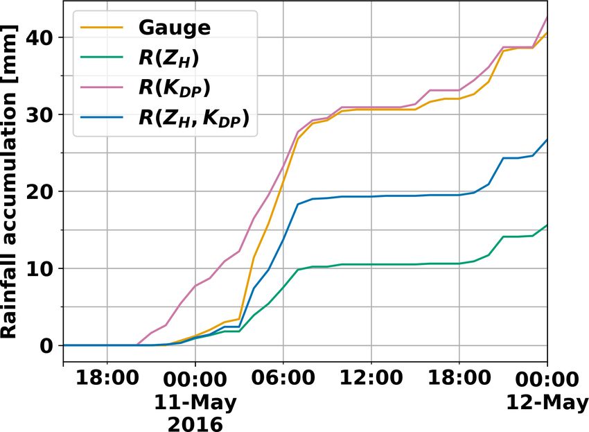
T. Voormansik et al.: Evaluation of the dual-polarization weather radar quantitative precipitation                                      1253

Figure 5. Scatter plots of radar-based rainfall estimates against rain gauge observations for 1 h accumulation intervals in Estonia 2011–2018.
The corresponding verification measures are presented in Table 3. The number of radar–gauge data pairs with eight gauges and accumulations
>0.1 mm is 7019. ZH is not corrected for attenuation.

Figure 6. The 1 h accumulations for Italy, 2012–2016. The corresponding verification measures are presented in Table 4. The number of
radar–gauge data pairs with 42 gauges and accumulations >0.1 mm is 1233. ZH is not corrected for attenuation.

Table 5. Verification of the radar-based rainfall 24 h accumulation      3.3    Comparison of 24 h accumulations
products of Estonia. ZH is not corrected for attenuation.

                               R          R      R(ZH ,                  Table 5 shows the verification results for the daily accumu-
                             (ZH )     (KDP )     KDP )                  lation interval in Estonia, while Fig. 7 presents the corre-
                                                                         sponding scatter plots. As expected, much less scatter can be
           CC               0.831      0.792      0.827
                                                                         seen than on the daily level, but overall, the results are con-
           NMAE             0.475      0.845      0.438
           NMB             −0.050      2.290      0.343                  sistent with the hourly interval verification outcomes. Using
           RMSE(mm)         4.366      7.195      3.992                  longer accumulation intervals leads to less severe errors as
           NASH             0.335     −0.097      0.392                  the longer period compensates for both underestimates and
                                                                         overestimates. The reflectivity-based product, R(ZH ), still
                                                                         underestimated rain depths, while the negative bias is consid-
                                                                         erably smaller than in hourly interval data. By looking at the
Table 6. Verification of the radar-based rainfall 24 h accumulation      definition of NMB in Eq. (3), it can be seen that in the case
products of Italy. ZH is not corrected for attenuation.                  that the same underlying samples are used, NMB should be
                                                                         equal on all accumulation lengths. In our study, the underly-
                               R         R      R(ZH ,                   ing samples were different as the 0.1 mm threshold was ap-
                             (ZH )    (KDP )     KDP )                   plied after the accumulation as the last step before calculating
                                                                         the verification metrics. This emphasizes the importance of
            CC              0.692      0.661     0.708
                                                                         low-intensity precipitation for total accumulations. R(KDP )
            NMAE            0.504      0.636     0.553
            NMB             −0.01      0.789     0.459                   is the least accurate of the three products, also on a daily
            RMSE(mm)        8.909     11.071    10.552                   accumulation level, with the lowest correlation and highest
            NASH            0.238      0.054     0.098                   error scores. The combined product, R(ZH , KDP ), removes
                                                                         the negative bias of R(ZH ) and shows better correlation and
                                                                         substantial improvement in terms of both the systematic er-
                                                                         ror and the overall error compared to R(KDP ). R(ZH , KDP )
                                                                         has the smallest NMAE of 0.438, a RMSE of 3.992 mm, and

https://doi.org/10.5194/hess-25-1245-2021                                               Hydrol. Earth Syst. Sci., 25, 1245–1258, 2021
1254 T. Voormansik et al.: Evaluation of the dual-polarization weather radar quantitative precipitation
the highest Nash–Sutcliffe efficiency, equal to 0.392. Overall Table 7. Verification of the radar-based rainfall monthly accumula-
there is noticeably less scatter in the daily radar accumula- tion products of Estonia. ZH is not corrected for attenuation.
tions compared to the 1 h interval.
Table 6 shows the verification results for the daily accumu- R R R(ZH ,
lation interval in Italy, while Fig. 8 presents the correspond- (ZH ) (KDP ) KDP )
ing scatter plots. R(ZH ) slightly underestimated accumula- CC 0.877 0.789 0.875
tions compared to gauge results, and surprisingly it outper- NMAE 0.360 0.822 0.214
forms other competing products in all metrics except Pear- NMB −0.284 1.042 0.109
son’s correlation coefficient. R(KDP ) again overestimated RMSE(mm) 27.448 62.466 16.704
accumulations the most and has the lowest correlation with NASH 0.155 −0.924 0.486
gauge data. R(ZH , KDP ) notably improves the R(KDP ) in all
verification metrics but does not exceed R(ZH ), except for
Table 8. Verification of the radar-based rainfall monthly accumula-
the correlation coefficient, which is the highest of all three tion products of Italy. ZH is not corrected for attenuation.
products with an r of 0.708. In Italy, the decrease in scatter of
radar accumulations cannot be observed compared to the 1 h R R R(ZH ,
level. In Fig. 7 two regimes can be observed, and we assume (ZH ) (KDP ) KDP )
that VPR correction leads to these regimes. Bric della Croce
weather radar is located on a top of a hill at 770 m a.s.l., and CC 0.776 0.726 0.799
NMAE 0.375 0.488 0.408
during the winter season, a vertical profile reflectivity cor-
NMB −0.128 0.310 0.337
rection (VPR) is applied (Koistinen, 1991). This correction
RMSE(mm) 23.737 30.802 24.914
is manually switched on at the beginning of the cold season, NASH 0.288 0.076 0.253
and it is switched off at the end. In the case of convective pre-
cipitation, this correction may lead to rainfall overestimation.
On the other hand, stratiform cold precipitation is heavily un-
metrics indicate better performance of the radar products on
derestimated when VPR correction is switched off.
a monthly scale compared to daily intervals. The correlation
coefficient is higher and the NMAE is lower for all the prod-
3.4 Comparison of monthly accumulations
ucts when the two timescales are compared.
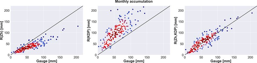
Table 7 shows the verification results for the monthly accu-
mulation interval in Estonia, while Fig. 9 presents the cor- 4 Conclusions
responding scatter plots. Compared to shorter timescales,
overall on a monthly scale the correlation of all the prod- In the present study polarimetric rainfall retrieval methods
ucts with gauge accumulations is higher. R(ZH ) underesti- for the fully operational C-band radars in Sürgavere, Estonia,
mated accumulations, with a larger mean bias (−0.284) than and Bric della Croce, Italy, have been analysed. The study
on a daily level but with a smaller normalized mean ab- focuses on the warm period of the year, and a long period of
solute error (0.360). R(KDP ) showed less scatter than on multi-year data is used. From Estonia 5 years of data from
shorter timescales like other products while it still heav- 2011 to 2018 has been included; from Italy, the data interval
ily overestimated accumulations (NMB equal to 1.042 with ranges from 2012 to 2016. Reflectivity data were calibrated
a RMSE equal to 62.466 mm). On the monthly accumu- following a self-consistency theory, and measured horizon-
lation level, R(ZH , KDP ) outperforms the two other prod- tal reflectivity (ZH ) was corrected accordingly. To calculate
ucts to a great extent. It is well correlated to gauge values rainfall from polarimetric variables, the differential propaga-
with small scatter as it performs very well, both in low- tion phase product (ØDP ) was reconstructed, and based on
and high-accumulation cases. The correlation coefficient is that the specific differential phase product (KDP ) was re-
nearly identical to R(ZH ), but it removes the systematic un- trieved. To achieve this the transparently implemented algo-
derestimation of R(ZH ) and overestimation of R(KDP ) and rithm phase_proc_lp (Giangrande et al., 2013) in the open-
exceeds them in all other verification metrics. source toolkit Py-ART was used for Estonian data. For Ital-
Table 8 shows the verification results for the monthly ac- ian data, KDP precipitation estimates were obtained follow-
cumulation interval in Italy, while Fig. 10 presents the corre- ing the theory set down in Wang et al. (2009).
sponding scatter plots. Scatter plots reveal similar character- Three radar rainfall estimation products were computed:
istics to the daily level accumulations of the products. R(ZH ) a horizontal reflectivity-based product R(ZH ), a specific
underestimated rainfall, also on a monthly scale, and R(KDP ) differential-phase-based product R(KDP ), and a combined
overestimated rainfall. R(ZH , KDP ) still overestimated rain- product based on the previous two R(ZH , KDP ). Rain gauge
fall but with a decreased RMSE compared to the R(KDP ) network data of Italy and Estonia were used as ground truth.
product. It also exhibits the highest correlation coefficient of The 1 h, 24 h, and monthly accumulations were derived from
the three. According to the verification results, most of the the radar products and gauge data.
Hydrol. Earth Syst. Sci., 25, 1245–1258, 2021 https://doi.org/10.5194/hess-25-1245-2021T. Voormansik et al.: Evaluation of the dual-polarization weather radar quantitative precipitation 1255
Figure 7. The 24 h accumulations for Estonia, 2011–2018. The corresponding verification measures are presented in Table 5. The number of
radar–gauge data pairs with eight gauges and accumulations >0.1 mm is 2148. ZH is not corrected for attenuation.
Figure 8. The 24 h accumulations for Italy, 2012–2016. The corresponding verification measures are presented in Table 6. The number of
radar–gauge data pairs with 42 gauges and accumulations >0.1 mm is 3010. ZH is not corrected for attenuation.
Time-series comparison revealed that even with a 15 min Overall the results show that the combined product
scan interval, radar is suitable for QPE, at least with more R(ZH , KDP ) performs better in almost all of the verification
widespread precipitation like stratiform rain. Still, on the measures in both countries compared to R(ZH ) and R(KDP )
shortest accumulation period of 1 h, the scarcer radar data as it successfully uses the benefits of each other product and
from Estonia had more scatter than data from Italy, where the eliminates the weaknesses. R(ZH ) was good at low precipi-
scan interval was 10 min on older data and 5 min since 2013. tation intensities, but in general, it underestimated precipita-
As an overall trend, the longer the accumulation period, the tion. It had an average NMB of −0.159 for all accumulation
less scattering that was visible. The case comparisons also lengths in Estonia and −0.145 in Italy. R(KDP ) performed
revealed the shortcomings of analysis based only on selected well at higher intensities but in general overestimated pre-
short periods. The performance of the QPE methods then de- cipitation. It had an average NMB of 1.731 for all the ac-
pends on the representativeness of the chosen cases, and re- cumulation lengths in Estonia and 0.592 in Italy, while the
sults can easily be skewed. Using a dataset with a length of at combined product R(ZH , KDP ) slightly overestimated pre-
least several years without preselection provides more robust cipitation, with an average NMB of 0.250 for all the accu-
results and allows for evaluating the operational usability of mulation lengths in Estonia and 0.305 in Italy. In both coun-
the methods. tries the R(ZH , KDP ) product also had the highest average
When the three products are compared to each other based CC over all the accumulation lengths, with CC of 0.800 in
on the full length of 5 years of data, in the case of Estonia, Estonia and 0.792 in Italy. Generally, the CC was higher the
the R(ZH , KDP ) was superior to R(ZH ) and R(KDP ) in all longer the accumulation period was, with the highest CC in
accumulation periods. Especially on the monthly accumula- monthly accumulations (R(ZH , KDP ) CC of 0.875 in Estonia
tion scale, it performed distinctly better as it had a RMSE and 0.799 in Italy).
39% lower than the nearest competitor, the R(ZH ) product, In Estonia, the overestimation of R(KDP ) was noticeably
and even 73% lower than R(KDP ). In Italy, the R(ZH , KDP ) higher than in Italy. We hypothesize that this is mostly due
product exceeded the two others clearly on an hourly level. to different climatological regimes between Italy and Esto-
On 24 h and monthly accumulation scale, it had the highest nia as high-intensity rainfalls occur more frequently in Italy,
correlation with gauge measurements, but the error verifica- although one has to keep in mind that the radars were from
tion measures were slightly higher than those of the R(ZH ). different manufacturers and thus also the KDP retrieval algo-
Nevertheless, it outperformed R(KDP ) on all timescales. rithms used were different, which might be the cause of some
discrepancy. Another source of error might originate from the
https://doi.org/10.5194/hess-25-1245-2021 Hydrol. Earth Syst. Sci., 25, 1245–1258, 20211256 T. Voormansik et al.: Evaluation of the dual-polarization weather radar quantitative precipitation
Figure 9. Monthly accumulations for Estonia, 2011–2018. The corresponding verification measures are presented in Table 7. The number of
radar–gauge data pairs with eight gauges is 179. ZH is not corrected for attenuation.
Figure 10. Monthly accumulations for Italy, 2012–2016. The corresponding verification measures are presented in Table 8. The number of
radar–gauge data pairs with 42 gauges is 675. ZH is not corrected for attenuation.
implemented ZH –R and KDP –R relations, which might not Competing interests. The authors declare that they have no conflict
perform equally in different climates. Overall the results of of interest.
the study showed that dual-polarimetric radar QPE and espe-
cially the combined product R(ZH , KDP ) show good poten-
tial to be used on long-term datasets if certain limitations are Acknowledgements. The authors are grateful to the Meteorological
considered. Observation Department of the Estonian Environment Agency for
Synoptic patterns could be used as an additional source for providing rain gauge datasets. The authors would also like to thank
editor Laurent Pfister, reviewer Hidde Leijnse, and two anonymous
classifying the radar accumulations. This would enable the
reviewers for their constructive comments that helped to signifi-
performance of each radar product to be verified for strati-
cantly improve the manuscript.
form and convective events. Moreover, it could be used to
investigate if frequent scans play a bigger role in convective
events than stratiform events as could be hypothesized and to Financial support. This research has been supported by the Esto-
quantify the effect. nian Ministry of Education and Research (grant no. IUT20-11), the
For future studies, it would also be useful to calcu- Estonian Research Council (grant no. PSG202), and the European
late probabilities and return periods of extreme rainfall for Regional Development Fund within the National Programme for
weather-radar-based rainfall climatology. Addressing Socio-Economic Challenges through R&D (grant no.
RITA1/02-52-07).
Code and data availability. The code used to conduct all analyses
in this paper is available by contacting the authors. Gauge and radar Review statement. This paper was edited by Laurent Pfister and re-
data used in this study are available by contacting the authors. viewed by Hidde Leijnse and two anonymous referees.
Author contributions. TV, RC, PP, and DM directly contributed to
the conception and design of the work. TV and RC collected and
processed the various datasets and wrote the original draft with in-
References
put from PP and DM. All authors reviewed and edited the final draft.
Alber, R., Jaagus, J., and Oja, P.: Diurnal cycle of pre-
cipitation in Estonia, Est. J. Earth Sci., 64, 305–313,
https://doi.org/10.3176/earth.2015.36, 2015.
Hydrol. Earth Syst. Sci., 25, 1245–1258, 2021 https://doi.org/10.5194/hess-25-1245-2021T. Voormansik et al.: Evaluation of the dual-polarization weather radar quantitative precipitation 1257
Bringi, V. N., Rico-Ramirez, M. A., and Thurai, M.: Rain- phase processing, J. Atmos. Ocean. Tech., 30, 1716–1729,
fall estimation with an operational polarimetric C-band radar https://doi.org/10.1175/JTECH-D-12-00147.1, 2013.
in the United Kingdom: comparison with a gauge net- Gorgucci, E., Scarchilli, G., and Chandrasekar, V.: Calibration of
work and error analysis, J. Hydrometeorol., 12, 935–954, radars using polarimetric techniques, IEEE T. Geosci. Remote,
https://doi.org/10.1175/JHM-D-10-05013.1, 2011. 30, 853–858, https://doi.org/10.1109/36.175319, 1992.
Cao, Q., Knight, M., and Qi, Y.: Dual-pol radar measurements Gorgucci, E., Scarchilli, G., and Chandrasekar, V.: A proce-
of Hurricane Irma and comparison of radar QPE to rain gauge dure to calibrate multiparameter weather radar using proper-
data, in: Proceedings of the 2018 IEEE Radar Conference, ties of the rain medium, IEEE T. Geosci. Remote, 37, 269–276,
Oklahoma City, OK, USA, 23–27 April 2018, 0496–0501, https://doi.org/10.1109/36.739161, 1999.
https://doi.org/10.1109/RADAR.2018.8378609, 2018. Goudenhoofdt, E. and Delobbe, L.: Generation and verifica-
Chandrasekar, V. and Cifelli, R.: Concepts and principles of rainfall tion of rainfall estimates from 10-yr volumetric weather
estimation from radar: Multi sensor environment and data fusion, radar measurements, J. Hydrometeorol., 17, 1223–1242,
Indian J. Radio Space, 41, 389–402, 2012. https://doi.org/10.1175/JHM-D-15-0166.1, 2016.
Chandrasekar, V., Keränen, R., Lim, S., and Moisseev, D.: Re- Gourley, J. J., Illingworth, A. J., and Tabary, P.: Abso-
cent advances in classification of observations from dual lute calibration of radar reflectivity using redundancy
polarization weather radars, Atmos. Res., 119, 97–111, of the polarization observations and implied constraints
https://doi.org/10.1016/j.atmosres.2011.08.014, 2013. on drop shapes, J. Atmos. Ocean. Tech., 26, 689–703,
Chang, W. Y., Vivekanandan, J., Ikeda, K., and Lin, P. L.: Quan- https://doi.org/10.1175/2008JTECHA1152.1, 2009.
titative precipitation estimation of the epic 2013 Colorado flood Gregorč, G., Macpherson, B., Rossa, A., and Haase, G.: As-
event: Polarization radar-based variational scheme, J. Appl. Me- similation of radar precipitation data in NWP Models–
teorol. Climatol., 55, 1477–1495, https://doi.org/10.1175/JAMC- a review, Phys. Chem. Earth Pt. B, 25, 1233–1235,
D-15-0222.1, 2016. https://doi.org/10.1016/S1464-1909(00)00185-4, 2000.
Chen, H. and Chandrasekar, V.: The quantitative precipita- Helmus, J. J. and Collis, S. M.: The Python ARM Radar Toolkit
tion estimation system for Dallas–Fort Worth (DFW) ur- (Py-ART), a Library for Working with Weather Radar Data in
ban remote sensing network, J. Hydrol., 531, 259–271, the Python Programming Language, J. Open Res. Softw., 4, e25,
https://doi.org/10.1016/j.jhydrol.2015.05.040, 2015. https://doi.org/10.5334/jors.119, 2016.
Cifelli, R., Chandrasekar, V., Lim, S., Kennedy, P. C., Koistinen, J.: Operational correction of radar rainfall errors due
Wang, Y., and Rutledge, S. A.: A new dual-polarization to the vertical reflectivity profile, Proceedings of the 25th
radar rainfall algorithm: Application in Colorado pre- Radar Meteorology Conference, American Meteorological So-
cipitation events, J. Atmos. Ocean. Tech., 28, 352–364, ciety, Paris, France, 91–96, 1991.
https://doi.org/10.1175/2010JTECHA1488.1, 2011. Krajewski, W. F., Villarini, G., and Smith, J. A.: Radar-
Cornes, R. C., van der Schrier, G., van den Besselaar, E. J., and Rainfall Uncertainties: Where are We after Thirty
Jones, P. D.: An Ensemble Version of the E-OBS Tempera- Years of Effort?, B. Am. Meteorol. Soc., 91, 87–94,
ture and Precipitation Data Sets, J. Geophys. Res.-Atmos., 123, https://doi.org/10.1175/2009BAMS2747.1, 2010.
9391–9409, https://doi.org/10.1029/2017JD028200, 2018. Lauri, T., Koistinen, J., and Moisseev, D.: Advection-Based Adjust-
Cremonini, R. and Bechini, R.: Heavy rainfall monitoring by ment of Radar Measurements, Mon. Weather Rev., 140, 1014–
polarimetric C-band weather radars, Water-Sui., 2, 838–848, 1022, https://doi.org/10.1175/MWR-D-11-00045.1, 2012.
https://doi.org/10.3390/w2040838, 2010. Leinonen, J., Moisseev, D., Leskinen, M., and Petersen, W.
Cremonini, R. and Tiranti, D.: The Weather Radar Obser- A.: A climatology of disdrometer measurements of rain-
vations Applied to Shallow Landslides Prediction: A Case fall in Finland over five years with implications for global
Study From North-Western Italy, Front. Earth Sci., 6, 134, radar observations, J. Appl. Meteorol. Climatol., 51, 392–404,
https://doi.org/10.3389/feart.2018.00134, 2018. https://doi.org/10.1175/JAMC-D-11-056.1, 2012.
Crisologo, I., Vulpiani, G., Abon, C. C., David, C. P. C., Macpherson, B., Lindskog, M., Ducrocq, V., Nuret, M., Gre-
Bronstert, A., and Heistermann, M.: Polarimetric rainfall re- goric, G., Rossa, A., Haase, G., Holleman, I., and Al-
trieval from a C-Band weather radar in a tropical environ- beroni, P. P.: Assimilation of Radar Data in Numerical
ment (The Philippines), Asia-Pac. J. Atmos. Sci., 50, 595–607, Weather Prediction (NWP) Models, in: Weather Radar – Prin-
https://doi.org/10.1007/s13143-014-0049-y, 2014. ciples and Advanced Applications, Springer, Berlin, Germany,
Devoli, G., Tiranti, D., Cremonini, R., Sund, M., and Boje, S.: Com- https://doi.org/10.1007/978-3-662-05202-0_9, 2004.
parison of landslide forecasting services in Piedmont (Italy) and Montopoli, M., Roberto, N., Adirosi, E., Gorgucci, E., and Baldini,
Norway, illustrated by events in late spring 2013, Nat. Hazards L.: Investigation of Weather Radar Quantitative Precipitation Es-
Earth Syst. Sci., 18, 1351–1372, https://doi.org/10.5194/nhess- timation Methodologies in Complex Orography, Atmosphere-
18-1351-2018, 2018. Basel, 8, 34, https://doi.org/10.3390/atmos8020034, 2017.
Giangrande, S. E. and Ryzhkov, A. V.: Estimation of rain- Nash, J. E. and Sutcliffe, J. V.: River flow forecasting through con-
fall based on the results of polarimetric echo classi- ceptual models part I: A discussion of principles, J. Hydrol., 10,
fication, J. Appl. Meteorol. Climatol., 47, 2445–2462, 282–290, https://doi.org/10.1016/0022-1694(70)90255-6, 1970.
https://doi.org/10.1175/2008JAMC1753.1, 2008. Overeem, A., Holleman, I., and Buishand, A.: Deriva-
Giangrande, S. E., McGraw, R., and Lei, L.: An applica- tion of a 10 year radar-based climatology of rain-
tion of linear programming to polarimetric radar differential fall, J. Appl. Meteorol. Climatol., 48, 1448–1463,
https://doi.org/10.1175/2009JAMC1954.1, 2009.
https://doi.org/10.5194/hess-25-1245-2021 Hydrol. Earth Syst. Sci., 25, 1245–1258, 2021You can also read