Feasibility Study for the Implementation of Algae Cell Monitoring in Raw Water Using an Optical Sonde at the Görväln Drinking Water Treatment ...

Rapport
Diarienummer Projektnummer
NV Rapport 2021-10 Examensarbete, 15 hp

Feasibility Study for the Implementation of Algae Cell
Monitoring in Raw Water Using an Optical Sonde at the
Görväln Drinking Water Treatment Plant
Examensarbete, Högskoleingenjörsexamen Kemiteknik, KTH

Louise Ulveland
KTH i samarbete med Norrvatten

2021-06-23

DEGREE PROJECT IN CHEMICAL ENGINEERING,
 FIRST CYCLE, 15 HP
 STOCKHOLM, SWEDEN 2021

 Feasibility Study for the
 Implementation of Algae Cell
 Monitoring in Raw Water
 Using an Optical Sonde at the
 Görväln Drinking-Water
 Treatment Plant

 LOUISE ULVELAND

KTH ROYAL INSTITUTE OF TECHNOLOGY
SCHOOL OF ENGINEERING SCIENCES IN CHEMISTRY,
BIOTECHNOLOGY AND HEALTH

DEGREE PROJECT
 Bachelor of Science in
 Chemical Engineering

Title: Feasibility Study for the Implementation of Algae
 Cell Monitoring in Raw Water Using an Optical
 Sonde at the Görväln Drinking-Water Treatment
 Plant

Swedish title: Genomförbarhetsstudie för implementering av
 algövervakning i råvatten med optisk sond vid
 Görvälnverket

Keywords: Algae Monitoring, Chlorophyll, Fluorescence

Workplace: Norrvatten

Supervisor at
workplace: Ewelina Basiak-Klingspetz

Supervisor at
KTH: Susanna Höglund Lenninger

Student: Louise Ulveland

Date: 2021-06-21

Examiner: Susanna Höglund Lenninger

Abstract
Each year, algae blooms occur in lake Mälaren in Stockholm and can cause complications in drinking-
water treatment plants. It is predicted that the risk for algae bloom in Mälaren will increase due to the
effects of climate change. To monitor levels of algae can be time consuming but installing an on-line
sensor for real-time monitoring can be beneficial and act as an early warning system. The aim of this
project is to support Norrvatten in their work to implement an automated early warning system for the
detection of cyanobacteria (aka blue-green algae), at their drinking-water treatment plant at Görväln.

In pursuit of this aim, the feasibility of using the EXO2 sensor was explored where chlorophyll was
measured as a proxy parameter for total algae. The study took 10 weeks where on-site data collection
was conducted, and validation of measurements was done by comparing data with laboratory results.
The EXO2 has potential to be used as a monitoring instrument for an early warning system for algae
bloom. It can measure chlorophyll concentrations above 10 μg/l in raw water at the Görväln plant with
a 95% confidence when correction factors are applied. The level of chlorophyll can furthermore be
translated to algae cell density which can be used as an indicator for total algae bloom. To maintain high
confidence in the chlorophyll measurements, the sonde should be checked once a week with a new
reference solution with known concentrations. This solution can be stored and used for one week,
maximum two depending on the composition of the solution.

Sammanfattning
Varje år sker det algblomning i Mälaren i Stockholm och kan orsaka svårigheter i reningsprocesser hos
vattenverk. Studier visar att risken för algblomning i Mälaren kommer att öka över åren på grund av
temperaturökning från klimatförändringen. Att installera en analysteknik, där man med en on-linesensor
detekterar alger kontinuerligt, skulle vara effektivare tidsmässigt än att räkna alger. En on-line sensor
skulle även kunna fungera som ett tidigt varningssystem för algblomning i Mälaren. Syftet med detta
projekt är att stödja Norrvatten i deras arbete med att implementera ett automatiserat system för tidig
varning för cyanobakterier (blågröna alger) vid Görvälnverket.

Möjligheten att använda EXO2-sensorn undersöktes där klorofyllhalten mättes som proxy för totala
alger. Studien tog 10 veckor där datainsamling genomfördes och validering av mätningar gjordes genom
att jämföra data från laboratorieresultat. EXO2-sensorn har potential att användas som för ett tidigt
varningssystem för algblomning. Det kan mäta klorofyllhalter över 10 μg/l i råvatten vid Görvälnverket
med 95% konfidens när korrigeringsfaktorer tillämpas. Nivån av klorofyll kan dessutom översättas till
densitet av algceller som kan användas som en indikator för total algblomning. För att upprätthålla högt
förtroende för klorofyllmätningarna bör sonden kontrolleras en gång i veckan med en ny referenslösning
med kända koncentrationer. Denna lösning kan lagras och användas i en vecka, högst två beroende på
lösningens sammansättning.

Acknowledgments
This project has been a real pleasure to work on and it is all thanks to the people who made it possible. I
want to first and foremost thank my supportive supervisor at Norrvatten, Ewelina Basiak-Klingspetz.
From introducing me to the world of municipal drinking-water treatment to bouncing ideas and
calculations with me. She was a great teacher who always made time for my questions and trusted me to
work independently. Thank you, Ewelina. Then I want to thank Stephan Köhler who has been like a
second supervisor for me. He has contributed with many ideas and suggestions during the project as well
as shared his passion for water research, which I was inspired by. He was a great support and was always
available to answer questions. Thank you, Stephan. I also want to thank Daniel Hellström who was my
first point of contact at Norrvatten. He recognized my passion for water early on and has supported it
throughout this project. I am grateful he took a chance on me, allowing me to do my project at Norrvatten.
Thank you, Daniel. Then I want to thank my supervisor at KTH, Susanna Höglund Lenninger. Even with
her busy schedule, she found time to support me by answering my questions, bouncing calculations with
me and encouraging my decisions. She allowed me to work independently and I felt her trust and support
throughout the project. Thank you, Susanna. Finally, I want to thank my friend and classmate Johnny
Hagelin, our weekly chats about our respective projects gave me many ideas and motivation during the
project. It was very rewarding to have a friend by my side, cheering me on.

Table of Contents
1 Introduction ........................................................................................................................................ 1
 1.1 Aim, Objective and Research Questions ...................................................................................... 2
2 Theoretical Background ..................................................................................................................... 3
 2.1 Chlorophyll in Algae ..................................................................................................................... 3
 2.2 Measuring Chlorophyll with Fluorescence ................................................................................... 4
 2.3 Calibration for Chlorophyll Fluorescence .................................................................................... 5
 2.4 Interferences and Other Parameters ............................................................................................ 6
3 Methodology ...................................................................................................................................... 8
 3.1 Data collection and Materials....................................................................................................... 8
 3.1.1 Reference Solutions ............................................................................................................. 9
 3.1.2 Full Factorial Experiment................................................................................................... 11
 3.1.3 Raw Water Sampling and Measurements ..........................................................................12
 3.1.4 UV measurement of chlorophyll sample ............................................................................ 13
 3.2 Data Processing and Analysis...................................................................................................... 13
 3.2.1 Temperature and turbidity correction ................................................................................14
 3.2.2 Statistical analysis of collected data ...................................................................................14
 3.2.3 Calculations for the full factorial experiment ..................................................................... 15
 3.2.4 Graphical comparison of collected data ............................................................................. 15
 3.3 Methods of Selection ...................................................................................................................16
 3.4 Reliability and Validity ................................................................................................................16
 3.5 Ethical Considerations ................................................................................................................16
 3.6 Limitations of the Study .............................................................................................................. 17
4 Results .............................................................................................................................................. 18
 4.1 Reference Solutions.....................................................................................................................19
 4.2 Precision of Measurements ........................................................................................................ 22
 4.3 Full Factorial Experiment .......................................................................................................... 22
 4.4 Geometric Mean Regression ...................................................................................................... 24
 4.5 Algae Cells as a Function of Chlorophyll .................................................................................... 26
 4.6 Chlorophyll stabilization using a MgCaO 3 Mg(OH)2 solution .................................................... 26
5 Discussion ........................................................................................................................................ 28
 5.1 Stability of Reference solutions .................................................................................................. 28
 5.2 Precision of EXO2 Measurements ............................................................................................. 28
 5.3 Variables with largest effect on chlorophyll concentration measurements ............................... 29
 5.4 Accuracy of the EXO2 measurements ........................................................................................ 29
 5.5 Quantifying of algae cells using chlorophyll concentrations ...................................................... 29
 5.6 Chlorophyll stability ................................................................................................................... 29
 5.7 Sources of Error and Suggested Improvements ......................................................................... 29
6 Conclusion ....................................................................................................................................... 30
References ................................................................................................................................................ 31
Appendix I. List of Materials ...................................................................................................................... I
Appendix II. Statistical calculations ......................................................................................................... II

Abbreviations
Colored Dissolved Organic Matter (cDOM)

Dissolved Organic Matter (DOM)

Drinking-Water Treatment Plants (DWTP)

Fluorescence Dissolved Organic Matter (fDOM)

Formazine Nephelometric Units (FNU)

Geometric Mean Intercept (GMI)

Geometric Mean Regression (GMREG)

Geometric Mean Regression Slope (GMS)

Inner Filter Effect (IFE)

Light-Emitting Diode (LED)

Parts Per Billion (ppb)

Quinine Sulfate Units (QSU)

Sustainable Development Goals (SDGs)

World Health Organization (WHO)

Water Tracer (WT)

1 Introduction

In 2015, all members states of the United Nations agreed on a global partnership for sustainable
development. The partnership, also known as the 2030 Agenda, is grounded in the Sustainable
Development Goals (SDGs) that act as aspirational goals for all UN member states to achieve. SDG
number six, Clean Water and Sanitation for All, is arguably one of the most fundamental goals of the
2030 Agenda as it has strong links to poverty reduction, access to education, gender equality and more
(WHO/UNICEF, 2017). SDG 6 highlights the importance of having access to safe drinking water but
also warns UN member states to be aware that drinking-water quality is at risk due to the impacts of
climate change such as the rise in temperature (UN-Water, 2018).

One of the recommended actions to maintain good water quality is to implement early warning systems
for contaminants. This way, operational measurements can be taken before there is an accumulation that
risk the efficiency of the water treatment. Some contaminants are more predicable than others, but
contaminants caused by seasonal variability, such as algae, are highly important to monitor as climate
patterns are changing and the global temperature is increasing (WHO, 2017).

General algae are not classified as toxic per se but where there is algae bloom, cyanobacteria (aka. blue-
green algae) can also be present as they grow in similar conditions. Cyanobacteria can produce and
release toxins into the water and cause health damage if ingested (Rapala et al., 2002). The World Health
Organization (WHO) recommend that drinking-water treatment plants (DWTP) monitor algae levels as
an indicator for both general biomass and cyanobacteria. The monitoring should take place at the raw
water intake as it can cause much damage to the primary steps in the treatment process (WHO, 2017).

Each year algae blooms occur in lake Mälaren in Stockholm. It is predicted that the lake’s temperature
will continue to rise as an effect of climate change which increases the risk for algae bloom (Ejhed,
2020). Algal blooms can cause filter blockages at DWTP and there is an increased risk of cyanobacteria
accumulating in the process water if there are no preventative measures taken.

Quantifying algae in water can be done by measuring cell density [no. cells/ml] or measuring the
chlorophyll concentration [μg/l] (Almuhtaram et al., 2018). Cell density measurement is often done
though a cell count using a microscope, which is time consuming and not very precise. Likewise, the
method for determining chlorophyl concentration is commonly done by using spectrophotometry, which
can also time consuming as the water sample needs to be filtered and processed (Kong et al., 2014). A
more time effective method of analysis is installing on-line monitoring for real-time data collection. The
main issue regarding this method is that calibration and the reliability of the measurements are highly
site specific and needs to be considered before installation (Bertone, Burford and Hamilton, 2018).

Norrvatten is a municipal association working with drinking water treatment and distribution. They
distribute drinking water to 14 municipalities in northern Stockholm, covering nearly 700 000 people.
Their treatment plant, Görväln, is located by lake Mälaren in Järfälla municipality. There they produce
nearly 1600 liters per second resulting in roughly 50 million cubic meters per year (Norrvatten, no date).
Norrvatten are part of a research project called DiCyano where universities, drinking-water treatment
plants and companies have come together to create a digital platform for algae data. The focus is on
cyanobacteria to better understand its growth due to climate change and evaluating how to implement
early warning systems at DWTP (DiCyano, 2021).

 1

1.1 Aim, Objective and Research Questions
The aim of this study is to support Norrvatten in their work to implement an automated early warning
system for the detection of cyanobacteria, at their DWTP at Görväln. The objective is to explore the
feasibility of using the optical sonde called EXO2 as the detection device and chlorophyll as the
parameter for the warning system. To explore this objective, the project is guided by the following
research questions:

 - How should the sonde be used for the detection and quantification of algae cells and how reliable
 are the measurements?

 - How often does the EXO2 sonde need to be calibrated and which variables have the largest effect
 on the measurement of chlorophyll concentrations?

 2

2 Theoretical Background

This chapter gives an overview of algae, why we measure chlorophyll-a, how to measure it and the
technical workings of the measurements.

2.1 Chlorophyll in Algae
Algae is a group term of aquatic eucaryotic plants. There are different types of algae, such as red, green
and blue-green, and one of the main properties they have in common is that they contain chloroplasts
which give them the ability to photosynthesize (Andersen, 2021). The main molecule for photosynthesis
inside the algae’s chloroplast is chlorophyll (Tanaka and Tanaka, 2019), which can be divided into five
categories of a,b,c,d and f. All categories of chlorophyll consist of a magnesium ligand structure but have
different end groups. The differences in the end groups make certain chlorophylls more or less
electronegative. These differences in chemical structure is what sets the categories apart and all
categories have their own unique absorption spectra. Chlorophyll-a absorbs blue and red light (Chen,
2014) and is the least electronegative and most common of the chlorophylls in photosynthetic biomass
(Hoober, Eggink and Chen, 2007). The structure of chlorophyll-a is shown in figure 1.

 Figure 1. Chemical Structure of Chlorophyll a
 (https://pubchem.ncbi.nlm.nih.gov/compound/12085802#section=2D-Structure)

Chlorophyll-a is the most common of the chlorophylls to measure when it comes to algae monitoring as
it exists in all types of algae (Kong et al., 2014). In regard to algae monitoring for the purpose of drinking-
water quality, the main algae of interest is cyanobacteria (aka. blue-green algae), which is one of the
many algae that contain chlorophyll-a (Rapala et al., 2002). Cyanobacteria can produce toxins that can
cause damage to the liver and gastrointestinal systems if swallowed. The WHO (2015) recommends that
even though not all cyanobacteria produce toxins, all should be considered as toxic. Cyanobacteria can
also, like any algae, cause filter clogging and prohibit coagulation in drinking-water treatment plants
(WHO, 2017).

The risk of cyanobacteria in drinking-water treatment plants is when there is excessive growth, or so-
called algal bloom (WHO, 2015). Blooms are a consequence of natural water circulation which impacts
the temperature of the water but also of heightened levels of nitrogen and phosphorus from human
activity, which cause eutrophication (Sellner, Doucette and Kirkpatrick, 2003). Climate change is also a
contributing factor to algae bloom as it changes temperature patterns and therefore water patterns
(Bertone, Burford and Hamilton, 2018). There are signs of this from lake Mälaren where there is an
increase in run-off to the lake, causing an increase in temperature which is favorable for blooms. Each
year, algae blooms occur during the summer season in lake Mälaren and it is predicted to become more
frequent with climate change (Ejhed, 2020).

 3

Monitoring of cyanobacteria can be done through measuring levels of chlorophyll-a, measuring levels
total phosphorous, taking a sample under a microscope (WHO, 2015) or measuring levels of the pigment
phycocyanin (Kong et al., 2014). Phycocyanin is a pigment-protein that is uniquely produced by
cyanobacteria and measuring it gives an indication of concentration of cyanobacteria, but not
concentration of toxins that could be present (Bertone, Burford and Hamilton, 2018). Measuring
chlorophyll-a will give a general measurement of total algal biomass as all photosynthetic algae contains
chlorophyll-a. However, while it’s a less specified indicator, this biomass also includes cyanobacteria
and with that chlorophyll-a can be used as a parameter for early warning systems for algal blooms (WHO,
2015). Chlorophyll-a will hereafter only be referred to as chlorophyll.

2.2 Measuring Chlorophyll with Fluorescence
Chlorophyll can be measured with an optical fluorescence sensor (YSI, 2015). Fluorescence is a
measurement of light being emitted from a molecule. All fluorescent molecules each fall into a specific
emission spectrum, making it possible for quantitative and qualitative analysis. The principle of the
measurement lies within the energy states of a molecule. When a molecule is met with a ray containing
enough energy, it can transition from its normal orbital ground state to an excited state. The excitation
itself is the absorption of the light source, which is a photon of energy exciting the electrons to a higher
orbital energy state (Royer, 1995). This excitation does not last long and the molecule will quickly
transition back between the energy levels to reach back to the ground state, so-called relaxation. During
this transition, a photon is emitted at a certain wavelength depending on the “path” the excited molecules
transition back on, se figure 2.

As the excitation and relaxation pathways are different, the photon absorbed compared to the photon
released will have different wavelengths, or different energies, and that is what can be measured. In other
words, a fluorescence sensor will measure the intensity of the emission (Harris, 2016). To measure
chlorophyll in a water sample, the EXO2 uses a light-emitting diode (LED) to emit a blue light of 470
nm to excite the chlorophyll molecules. The emission from the excited chlorophyll is at 685 nm in the
form of a red light, which is registered by the sonde (Smith, 2018).

 Relaxation
Excited State
 Energy

 Absorption
 & excitation Fluorescence
 emission

 Ground State

 Figure 2. Fluorescence depicted through excitation and emission. Based on Harris (2016), p.446

 4

2.3 Calibration for Chlorophyll Fluorescence
To calibrate the EXO2 for chlorophyll measurements, the red dye, Rhodamine Water Tracer (WT)
(2,5%), is used as a secondary calibration standard (YSI, 2015). Like chlorophyll, Rhodamine is also a
fluorescent molecule and is shown in figure 3.

 Figure 3. Chemical Structure of Rhodamine WT
 (https://pubchem.ncbi.nlm.nih.gov/compound/Rhodamine-WT#section=2D-Structure)

Reason for using Rhodamine instead of a primary standard of the actual chlorophyll pigment is that
Rhodamine WT is relatively more stable and not too costly (Smith, 2018). Rhodamine is soluble in water
and a commonly used dye for fluorescent water measurements, the WT in the same even stands for
“Water Tracer” (Smith, 2020). Rhodamine is easy to detect by sensors as well as falls in a unique
fluorescence spectrum what covers only a select group of molecules normally found in water, narrowing
the risk of interferences. The excitation spectrum is around 558 nm and emission around 582 nm se figure
4 (Wilson, Cobb and Kilpatrick, 1986). These spectra covers the same spectra of both chlorophyll and
phycocyanin, where excitation is at 590 nm and emission at 685 nm, same emission as chlorophyll
(Smith, 2018).

 5

Rhodamine WT
 Excitation spectrum Emission spectrum
 (peak 558 nm) (peak 582 nm)

 Chlorophyll excitation with Chlorophyll emission (685 nm)
 blue light (470 nm)

Figure 4. Excitation and emission spectrum of calibration solution, Rhodamine WT (Based on Wilson, Cobb and
Kilpatrick, 1986), along with excitation and emission wavelengths for chlorophyll (Smith, 2018).

2.4 Interferences and Other Parameters
Known factors which can influence fluorescence measurements in water are turbidity, pH, quenching
and so-called inner-filter effects (Brand and Johnson, 2000). Temperature has shown to change the
fluidity of the membrane lipids of chloroplasts which consequently impacts fluorescence of chlorophyll
inside. Reasoning behind this phenomenon is believed to be due to the hydrophilic end of the chlorophyll
will have different mobility in the membrane when it’s colder as the fluidity of the membrane is more
crystalline (Murata and Fork, 1975). Temperature has also shown to have an inverse relationship with
fluorescence, which also could be a consequence of the chlorophyll mobility, but it is said to also be due
to general algae structure. In other words, as the temperature increases, the concentrations from the
fluorescence readings decreases (Smith, 2018).

Turbidity can interfere with the light from the sensor as well as the light emitted from the excited
molecule. The higher turbidity, the higher risk the light will scatter and interfere with the fluorescence.
To mitigate this, the manufactures of the EXO2 sonde recommend to simultaneously measure the
turbidity with an attached turbidity sensor as chlorophyll measurements are being made (Smith, 2018).
Another interference is the Inner Filter Effect (IFE). It is similar to interference caused by turbidity, but
instead of blocking the light, IFE is when other particles absorb the light, impacting the fluorescence
measurement (Brand and Johnson, 2000). These particles that can absorb the emitted light from an
excited molecule are called quenchers and they too can be fluorescent and give off their own emission.
Therefore, it’s recommended to verify measurement results with laboratory measurements as well
(Smith, 2018).

Dissolved organic matter (DOM) exists in all raw water in various compositions of molecules but is
mainly defined as dissolved organic carbon but also nitrogen, phosphorus and sulfur. DOM can be
divided into two categories, separated by spectroscopic measurements where colored DOM (cDOM)
which absorbs ultraviolet light and then there is fluorescence DOM (fDOM) which is the organic matter
that is fluorescent (Hartnett, 2018). Both can be used for measuring DOM but in this project fDOM is
the parameter used. To calibrate a fDOM sensor, quinine sulphate is used as its excitation wavelength is

 6

365 nm and emission is around 480 nm, which covers the spectra for DOM. The unit for fDOM is most
commonly expressed in Quinine Sulfate Units (QSU), which is defined as parts per billion (ppb) quinine
sulfate (YSI, 2015).

A part from fDOM, turbidity is an essential parameter to measure as it can interfere with the chlorophyll
measurements (Smith, 2018). Turbidity is a measurement of how light scatters due to suspended
particles, in other words, it’s a measurement of the transparency of the water (WHO, 2017). Turbidity is
usually defined in formazine nephelometric units (FNU) and drinking-water in Sweden has a limit of 0,5
FNU, above that is no longer considered as potable water (Livsmedelsverket, 2017). A sensor can be
calibrated by using a formazine standard solution but also polymer-based solutions are being used (YSI,
2015). Furthermore, measuring the water’s pH is also important where NaHCO3 is commonly used as a
pH buffer (PubChem, no date). The EXO2 sensor uses an pH electrode containing a Ag/AgCl reference
electrode and a glass electrode to measure the difference in potential (YSI, 2015).

 7

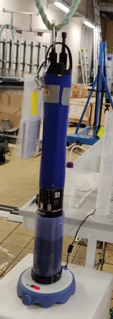
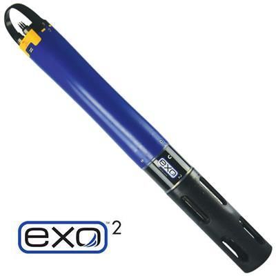
3 Methodology

The study took 10 weeks and was approached from three different fronts: a literature review, on-site data
collection and data analysis. All three components were addressed during a regular week where three
days would be spent on literature review and data analysis and the remaining days would be for on-site
data collection. The literature review consisted of a desk study based on evaluating scientific articles,
published reports and technical briefs on research pertaining to algae monitoring, sensor optimization,
validation of analysis and drinking-water quality. The research site for data collection took place at
Norrvatten’s DWTP, Görväln. It is located in Järfälla municipality, right next to lake Mälaren, where the
raw water samples were taken from. Data collection took place once to twice a week for five weeks. All
collected data were quantitative measurements using the YSI EXO2 water quality optical sonde, for more
details see 3.1 Data Collection and Materials.

The first research question pertains to the detection and quantification of algae cells using the sonde as
well as the reliability and validity of the measurements. As the sonde does not quantity number of cells
per se, the concentration of chlorophyll is measured as a proxy parameter. To test the validity of the
chlorophyll measurements [μg/l], water samples were sent to an external laboratory, Eurofins, to confirm
the concentration. Furthermore, the measurements were also compared to Norrvatten’s own laboratory
results where cell density [106cells/l] was counted. To test if the EXO2 data can act as an early warning
system, the collected data was also uploaded to Norrvatten’s data management system aCurve (Germit
Solutions, Sweden) where alerts were put in place for when the chlorophyll concentrations in the raw
water would reach certain limits.

The second research question focuses on the frequency at which the sonde needs to be calibrated.
Calibration frequency is defined through the use of reference solutions. The intended purpose of the
solutions is to act as verification of the sonde’s calibration settings by simply measuring the chlorophyll
concentration and comparing it to a standard solution, aka reference solution. The calibration frequency
will then be defined by how long these reference solutions can be stable for, in other words, how long
until the change in chlorophyll concentrations become statistically significant. To further explore how
and why the reference solutions change over time, a full factorial experiment was done, for more details,
see section Data Collection and Material.

3.1 Data collection and Materials
Data collection was divided into three parts;

 1. Measuring reference solutions over time to evaluate the stability of the solutions;

 2. A full factorial experiment to see which variable has the largest effect on the measurement of
 chlorophyll concentrations;

 3. Measuring chlorophyll concentrations in raw water at the Görväln DWTP;

The materials used for this study are listed in appendix I. The main analysis instrument was the EXO2
(YSI EXO2 599502-00, USA) which is a multiparameter sonde that can simultaneously measure pH,
temperature, turbidity, chlorophyll and other water quality parameters. Measurement data is
automatically stored in the sonde and can periodically be transferred in a CSV-file to a computer via
Bluetooth for further interpretation and analysis (YSI, 2015). Figure 5 shows the EXO2 with the
protective casing at the end. Underneath the casing are seven available ports to place different sensors,
along with a wiper that can clean the tips of all the sensors. The sensor is roughly 70 cm long, with a 7,6
cm diameter and weights 3,6 kg.

 8

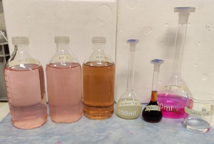
Figure 5. EXO2 Multiparameter Sonde (YSI, 2021)

The EXO2 sonde that was used for this project was calibrated by Norrvatten in accordance with the user
manual where 5 ml of the Rhodamine WT (2,5%) solution was taken out and filled to 1000 ml with
distilled water, giving a concentration of 125 mg/L. In turn, 5 ml of this solution was taken out and filled
to 1000 ml, giving a solution of 0,625 mg/L. This solution was then used for a calibration of chlorophyll
[μg/l] using the relationship in table 1 (YSI, 2015).

Table 1. Temperature's [°C] relationship to chlorophyll measurements [μg/l] at a rhodamine concentration at
0,625 mg/l.

 Solution
 Temperature 30 28 26 24 22 20 18 16 14 12 10 8
 [°C]

 (Rhodamine
 0,625 mg/l)
 56,5 58,7 61,3 63,5 66 68,4 70,8 73,5 76 78,6 81,2 83,8
 Chlorophyll
 [μg/l]

3.1.1 Reference Solutions
The purpose of the reference solutions is to act as a calibration check for the EXO2 sonde and reason for
testing them over time is to see how long a solution can be stored for. During the first week of data
collection, three reference solutions were prepared and labeled REF 1, REF 2 and REF 3. The solutions
contained different levels of rhodamine, bentonite, NaHCO3, Coca-Cola and distilled water. Rhodamine
was for chlorophyll measurements, bentonite for turbidity, NaHCO3 as a pH buffer and then to mimic
fDOM in, decarbonated Coca-Cola was used (Köhler, 2021). For details see table 2.

Table 2. Composition of the three reference solutions (REF 1, 2, and 3).

 Coca-Cola
 NaHCO3 Bentonite Rhodamine Distilled Total
 Solution (diluted
 (1 M) (5 g/l) (180 μg/l) water volume
 0,2 times)
 REF 1 100 ml 30 ml 5 ml 75 ml 790 ml 1000 ml
 REF 2 100 ml 10 ml 20 ml 75 ml 795 ml 1000 ml
 REF 3 300 ml 30 ml 0 ml 75 ml 595 ml 1000 ml

 9

3.1.2 Preparing and measuring the reference solutions
During the first week of data collection, 2000 ml of each reference solution was prepared. During the
course of data collection phase, these bottles were stored in a refrigerator at 3°C and taken out once a
week for measurements. Figure 6 shows the three reference solutions (REF 1, 2 and 3) as well as their
ingredients.

 Bentonite (5 g/l)
 REF 1 REF 2 REF 3

 Rhodamine (180 μg/l)

 Coca-Cola
 (diluted 0,2 times)

 NaHCO3 (1M)

 Figure 6. Reference solutions (REF 1, 2,and 3) were prepared with different concentrations of bentonite for
 turbidity, Coca-Cola for fDOM and NaHCO3 as a pH buffer. Levels of rhodamine were constant in the three
 solutions for chlorophyll measurements.

The EXO2 was hung up by rope and each sample was measured using the sonde’s own calibration cup.
Reason for this is the calibration cup has a blue tint and may block out some of the light in comparison
to a transparent, colorless beaker. Before each measurement, the sensors on the sonde and calibration
cup were rinsed with distilled water and the sensors were wiped clean by the sonde’s own brush system.
A magnet was placed inside the protective casing and the sonde was placed over a stirrer, see figure 7
for the setup.

 EXO2 sonde

 Calibration cup used for
 measuring samples

 Magnetic stirrer

Figure 7. Measurement set-up with the EXO2 sonde, its blue calibration cup for samples and a magnetic stirrer.

 10

The calibration cup was rinsed with the reference solution twice before the reference solution was poured
in to the first line on the cup, which is roughly 400 ml. The magnet stirrer was set to 300 rpm and the
sonde was left for one minute for the sensors to adjust to the sample before recording the data. For each
reference solution, 15 measurements were recorded, taken at one second apart.

Each week, a new reference solution was prepared in the same way as the original solutions and labeled
REF 1*, REF 2* and REF 3*. Measurements of these solutions was conducted using the same method
as the original solutions made the first week of data collection. The data of both the original reference
solutions and the weekly solutions were compared with each other to check the stability of the
chlorophyll concentration over time and to see how the solution changes, see section 4 Results.

3.1.3 Full Factorial Experiment
To assess which variables have the largest effect on the measurements of the chlorophyll concentrations,
a full factorial experiment was conducted. The purpose of a full factorial experiment is to evaluate
selected variables individually as well as combined to see if there is an effect and how large it is. The
outcome in this experiment is the concentration of chlorophyll. The selected variables are fDOM, pH
and turbidity. The different trials, or sample solutions, consisted of high and low levels of these three
variables, while the concentration of chlorophyll was kept constant in all trials. All four parameters were
measured simultaneously using the same measuring method as for the reference solutions, se description
above. As there were three variables with two levels, it’s was a so-called 23 full factorial experimental
design, meaning eight trials were needed as 23= 8 (Blomqvist, 2017). The variables were fDOM, pH and
turbidity and the eight trial solutions were based on the same “recipe” as the reference solutions where
chlorophyll was measured to 75 ml of rhodamine and low/high levels of the variables were added and
filled to 1000 ml with distilled water. Table 3 specifies the volume of each variable and level. Each trial
sample was prepared and immediately measured and all samples were measured 14 times.

 Table 3. List of variables and the volumes defining their low and high level.

 Low level High level
 Variable
 (-1) (1)
 A: fDOM 100 ml 300 ml
 B: pH 10 ml 30 ml
 C: Turbidity 5 ml 20 ml

 11

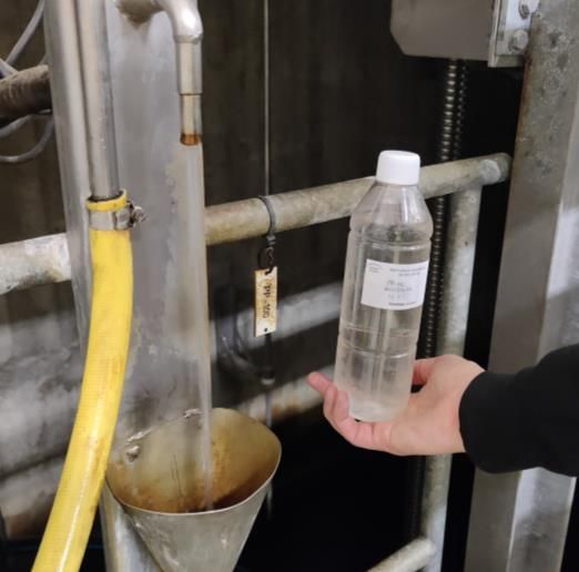
The design matrix is presented in table 4, where “-1” signifies a low level of a variable and “1” a high
level. With three variables at two levels, all combinations are covered in these eight trials.

 Table 4. Design Matrix for the Full Factorial Experiment detailing levels for each trial (low -1 and high 1).

 Trial A B C
 1 -1 -1 -1
 2 1 -1 -1
 3 -1 1 -1
 4 1 1 -1
 5 -1 -1 1
 6 1 -1 1
 7 -1 1 1
 8 1 1 1

3.1.4 Raw Water Sampling and Measurements
The raw water data was collected once a week where the EXO2 was submerged in the water overnight,
recording chlorophyll concentrations every 20 minutes. The measurement site is called PP100 and is
placed after a primary filtration of the raw water but it is still considered as raw water. The water samples
were taken the following day, at the same location. Using two sample bottles of 500 ml each, water was
collected from a tap pouring from the PP100 point, se figure 8.

 Figure 8. Sample bottle of 500 ml at sample collection site called PP100. Raw water coming out the tap for
 collecting raw water.

 12

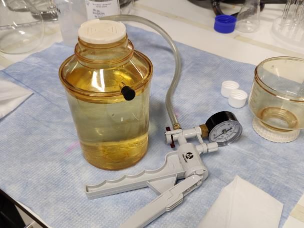
Each sample bottle was rinsed with the sample water twice before filling up the bottle. Immediately after
sampling, the 1000 ml of the sample was measured out in a volumetric flask. Three milliliters of 1%
MgCaO3 Mg(OH)2 solution was added to the 1000 ml sample. The water sample was then filtered through
a suction filtration apparatus using a 47 mm filter (Whatman GF/C, VWR 513-5227) and a handheld
pump, se figure 9. The filter was then removed from the filter head using plastic tweezers and folded
once in the middle with the filtered particles on the inside. To remove excess water the folded filter was
first placed on paper towels followed by a being placed in a plastic container containing silica beads. The
sample was frozen until shipped to the Eurofins laboratory where the levels of chlorophyll would be
measured in accordance with SS 028146-1. In this standardized spectrophotometric method, chlorophyll
is first extracted with acetone followed by absorbance measurements at 664, 647 and 630 nm (SIS, 2004).

 Figure 9. Suction filtration apparatus with handheld pump used to filter raw water samples to collect biomass
 on filter paper.

3.1.5 UV measurement of chlorophyll sample
The purpose of adding MgCaO3 Mg(OH)2 solution to the raw water sample is to stabilize the Mg-ligand
of the chlorophyl molecules. To test the difference in stability, a quick UV-measurement was conducted.
Two samples from PP100 were taken where one sample was processed as described above with adding
three milliliters of MgCaO3 Mg(OH)2 solution, and the other sample was processed the same way but
without the added solution. Each sample was run though a UV spectrometer (PerkinElmer LAMBDA
365, USA) at 254 nm at 1000 RPM for 400 seconds.

3.2 Data Processing and Analysis
Measurements collected at PP100 were stored in the EXO2 until transferred to a laptop via Bluetooth.
The data first appears in the sonde’s software, KorEXO, but can be downloaded as a CSV. file. All raw
data files were transferred directly into the data management software, aCurve. A copy of the data was
also made for analysis in Microsoft Excel. To make the files more manageable in Excel, the files were
trimmed leaving only data of the following list:

 - Date (MM/DD/YYYY)
 - Time (HH:MM:SS)
 - Site Name
 - Chlorophyll (µg/l)
 - fDOM (QSU)

 13

- Turbidity (FNU)
 - pH
 - Temperature (°C)
All collected data was compiled in Excel where statistical calculations (see section 3.2.2) were conducted
as well as compared graphically (see section 3.2.3) to identify patterns and potential correlations between
the collected data of the parameters listed above.

3.2.1 Temperature and turbidity correction
The raw data of Chlorophyll and fDOM measurements were then processed in Excel with correction
factors to account for temperature, turbidity and IFE. The correction factors and equations are based on
previous research and empirical data (Köhler, 2021). Equation 1 shows the temperature correction for
the chlorophyll measurements. Equations 2 corrects for fDOM absorbance which occurs at 254 nm.
Equation 3 and 4 accounts for the temperature as well as the turbidity of the fDOM readings. Finally,
equation 5 corrects for possible IFE, resulting in the final fDOM value used to data analysis. The
reference temperature (TempRef) is set to 25°C.

 ChlorophyllTemp = ChlorophyllEXO + ChlorophyllEXO ∙ 0,015(TempEXO − TempRef ) (Eq. 1)

 fDOMEXO
 fDOMA254 = 1 + (Eq. 2)
 3,5

 fDOMTemp = fDOMEXO + fDOMEXO ∙ 0,012(TempEXO − TempRef ) (Eq. 3)

 fDOMTemp
 fDOMTemp & Turb = −0,004687∙Turbidity + 0,3041 ∙ e−0,0003624∙TurbidityEXO (Eq.4)
 0,7225∙e EXO

 fDOMA254
 fDOMTemp,turb & IFE = fDOMTemp & Turb + fDOMTemp & Turb ∙ 0,2508 ∙ (Eq. 5)
 100

3.2.2 Statistical analysis of collected data
The purpose of the reference solutions was to see how long they can be stored for if they are stored in a
dark refrigerator. Original reference solutions (REF, 1 2 and 3) were created first week of data collection
and tested once a week for five weeks. They were also compared to newly made reference solutions
(REF 1*, 2* and 3*). The hypothesis is a statistical analysis can be used to evaluate when the chlorophyll
concentrations deviate too much from each other which indicates either the stability of the solutions is
questionable or the EXO2 needs to be recalibrated. To statistically evaluate this, a F-test and a t-test were
conducted. An F-test compares standard deviations between two measurements and a t-test is to see when
the standard deviations become significantly different. The F-test was only done on the measurements
that showed the greatest standard deviation in comparison to the other measurements. The F-test is based
on two values, Fcalculated and Ftable. If Fcalculated > Ftable then the difference in measurements is significant
and the measurement should be rejected. Equation 6 shows how Fcalculated was calculated. All statistical
equations are from Harris (2016).

 s2
 Fcalculated = s12 (Eq. 6)
 2

In order to calculate Fcalculated, one must first calculate the standard deviation, s. The formula “=STDEV”
was used in Excel to where the equation 7 is used to calculate the standard deviation. Equation 8 shows
the spooled standard deviation which is a term for a set of several standard deviations pooled together.
The spooled was used in the F-test to compare one measurement with the rest of the set.

 14

∑(xi−x̅)2
 sx = √ (Eq. 7)
 n−1

 2 s21 +s22 +s23 +⋯
 spooled = (Eq. 8)
 Nset

To get the Ftable value, the formula “=F.INV.RT” was used with a 95% confidence interval and the
corresponding degree of freedom to the data being analyzed. The Degrees of freedom is defined by
equation 9.

 Degrees of freedom = n1 + n2 + n3 + ⋯ − Nset (Eq. 9)

As for the t-test, if tcaclulated > ttable it means the change is significant with a 95% confidence interval. For
the t-test, equation 10 was used, along with equation 8 for spooled.

 |x̅ −x̅2 | n1 ⋅n2
 t calculated = s 1 √n (Eq. 10)
 pooled 1 +n2

To evaluate the precision of the measurements, equation 11 was used. This equation accounts for errors
by rejecting the 2,5th percentile, and putting the 95th percentile in relation to the median. This resulting
in an understanding of the variance in the measurements.

 (97th percentile−2,5thpercentile)
 95% within rage of the median = (Eq. 11)
 Median

3.2.3 Calculations for the full factorial experiment
The purpose of a full factorial experiment is to determine the effects of the variables of interest. To
calculate the main effects, β1, β2, and β3, as well as the interaction effects β4- β7,equation 12 was used
where the +/- was determined on whether it was a high (+) or low (-) level and m= number of trails,
which is eight.
 ̅1 ±y
 ±y ̅2 ±y
 ̅3 …±y
 ̅7
 βi = (Eq. 12)
 m

As there are multiple measurements, a pooled standard deviation was calculated using equation 8. A 95%
confidence interval was calculated using equation 13.

 ts
 x̅ ± (Eq.13)
 √n

3.2.4 Graphical comparison of collected data
In order to compare the EXO2 chlorophyll measurements in the raw water from the EXO2 with the
results from the Eurofins laboratory, the data was first tabulated where differences and quotients were
calculated. The data was then graphically compared doing a geometric mean regression (GMREG). The
method is grounded in a cross-comparison where the variables on the x-axis are seen as independent and
the variables on the y-axis as dependent. Two graphs were made titled adaptation 1 and 2 where the
adaptation 1 had EXO2 results was on the x-axis and the Eurofins results on the y-axis and vice versa
for adaptation 2. Using these two graphs, a combined linear relation could be calculated in the form of a

 15

geometric mean regression slope (GMS) and geometric mean intercept (GMI) could be calculated using
equation 14 and 15.
 1/2
 k
 GMS = (k adptation 1 ) (Eq.14)
 adaptation 2

 GMI = y̅Eurofins − GMS(x̅EXO ) (Eq. 15)

Using the GMS and GMI, a GMREG line can be defined by the equation 16 and was applied to the data
from adaptation 1, for full GMREG graph, see section 4 Results.

 GMREG = GMS ∙ x + GMI (Eq.16)

To compare the EXO2 measurements with the cell count from the laboratory, a t-test (Eq. 10) was done
to compare the difference with a 95% confidence interval. The results were then put in a Log-Log plot
to identify a potential correlation.

3.3 Methods of Selection
The location for the raw water sample, PP100, is the same location where Norrvatten’s laboratory take
their samples for algae cell count where they count number of cells under a microscope. As chlorophyll
measurements were to be compared with laboratory results, PP100 therefore seemed like most
appropriate location. The data collection (see detailed list in section 3.1.) took place once or twice a week
for five weeks and these were weeks 14-18 (April 5-May 7, 2021). The weeks for data collection were
selected in regard to the timeline for algae bloom as it usually starts around April-May in lake Mälaren
(Basiak-Klingspetz, 2021). Then the compositions of the reference solutions were put forward by
Norrvatten to mimic relevant paraments of the raw water.

3.4 Reliability and Validity
Validation of the PP100 measurements was done through sending a filter sample to the Eurofins
laboratory in accordance with the Swedish Standard, SS 028146-1. The results took roughly 3 business
days after arrival to the lab and the chlorophyll concentration was defined in μg/l. To determine the
reliability of the collected data, a series of statistical calculations were conducted in Excel, using a 95%
confidence interval. For list of calculations, se section Statistical Analysis.

3.5 Ethical Considerations
The project took place during the COVID-19 pandemic, which meant following the recommendations
put forth by the Public Health Agency of Sweden as well as Norrvatten’s own COVID-19 protocol.
Compliance was of utter importance as data collection took place at the Görväln plant where they produce
drinking-water for nearly 700 000 people (Norrvatten, no date). Being on-site also meant access to
sensitive information regarding the plant and in certain areas photographs were not allowed to be taken.
This was taken into consideration when photographing the data collection process and all photos have
been approved by Norrvatten.

 16

3.6 Limitations of the Study
The project is framed around chlorophyll measurements using the EXO2 sonde. All water sample data
is location specific and limited to PP100 at the Görväln plant. The data is also limited to the specific
EXO2 sonde that was used during the project. If this project were to be replicated using another EXO2
sonde, it would preferably be calibrated the same way and measurement data would be compared to see
that the signal is the same between the sondes.

The scope of the measurements was limited to investigate

 1. How the chlorophyll concentration relates to number of algae cells;

 2. How reliable the chlorophyll measurements are;

 3. What factors impact the chlorophyll measurements the most and;

 4. How often does a calibration solution need to be prepared.

 17

4 Results

In the section, the results from the reference solutions and the full factorial experiment will be presented
along with the evaluation of measurement accuracy, as well as the graphical comparisons between EXO2
with Eurofins and algae cell count. The chlorophyll and fDOM were corrected in accordance with
equations 1-5 prior to any statistical calculations. All statistical calculations can be found in Appendix II
and table 5 summaries the samples which have been studied along with their purpose and how the data
was analyzed.

Table 5. List of all data collected, which parameters were recorded, during what time period as well as the
purpose of the measurements and the method of data analysis.

 Results
 Parameters Method of
 Samples Time period Purpose of data found in
 recorded data analysis
 section

 Reference Chlorophyll (µg/l) 5 weeks with Evaluate when the F-test and t- 4.1
 solutions measurements chlorophyll test
 fDOM (QSU)
 once a week. concentrations (eq. 6-10)
 Turbidity (FNU) deviate too much
 pH from each other.

 Temperature (°C) Evaluate the Comparing 4.2
 precision of the the 95th
 measurements. percentile in
 relation to
 the median
 (eq. 11)

 Solutions Chlorophyll (µg/l) Data for the Evaluate which Calculating 4.3
 for full full factorial variable has the effect size
 Temperature (°C)
 factorial experiment largest effect on the and error
 experiments was collected measurement of bars
 in one day. chlorophyll (eq. 12, 13)
 concentrations.

 Raw water Chlorophyll (µg/l) 5 weeks with Evaluate accuracy of Geometric 4.4
 measurements EXO2 data by mean
 Temperature (°C)
 once a week. comparing EXO2 regression
 data with laboratory (eq.
 results. 14,15,16)

 Identify correlation Log-Log plot 4.5
 between EXO2 data and t-test
 on Chlorophyll with (eq. 10)
 number of algae
 cells.

 Measured once Test the stability of Percentage 4.6
 using the UV- chlorophyll from the difference
 spectrometer added MgCaO3
 solution.

 18

4.1 Reference Solutions
Chlorophyll, fDOM, turbidity and pH were observed over five weeks. Measurements were taken for all
three reference solutions (REF 1, 2, and 3) along with the newly created solutions (REF 1*, 2*, and 3*).
In REF 1, chlorophyll did not remain stable over time, as is shown in figure 10. The level of turbidity
and pH also changed over time where pH steadily decreased by each week (Fig. 13) and turbidity
fluctuated (Fig. 12). The only parameter that remained stable in comparison to the new weekly reference
solution (REF 1*) was fDOM. The fDOM level dipped in the first week and then flattened out, se figure
11. Statistical calculations (Eq. 6-10) show that there is significant change (95% confidence) to the levels
of chlorophyll already after one week meaning REF 1 cannot be stored over time. Measurement points
that are statistically significant are marked with an asterisk, *.

 Chlorophyll REF 1 fDOM REF1
 20.00 45.00
 Chlorophyll [ug/L]

 18.00 * *

 fDOM [QSU]
 40.00
 16.00 * *
 35.00
 14.00
 12.00 30.00

 10.00 25.00
 1 2 3 4 5 1 2 3 4 5
 Week Week

 Original REF 1 New REF 1* Original REF 1 New REF 1*

Figure 10. Chlorophyll concentration [µg/l] in solution REF 1 Figure 11. fDOM [QSU] in REF 1. Original REF 1 was a
where points marked with * are statistically significant. solution prepared the first week of data collection and a
Original REF 1 was prepared the first week of data collection new solution was prepared each week, labeled New REF1*.
and a new solution was prepared each week, labeled New The level of fDOM remains fairly constant over the weeks
REF1*. The concentration of chlorophyll fluctuates over time indicating this parameter can remain stable for four
indicating the chlorophyll is not stable. weeks.

 Turbidity REF 1 pH REF 1
 10.00 8.50
 Turbidity [FNU]

 8.00 8.00
 7.50
 6.00
 pH

 7.00
 4.00
 6.50
 2.00 6.00
 0.00 5.50
 1 2 3 4 5 1 2 3 4 5
 Week Week

 Original REF 1 New REF 1* Original REF 1 New REF 1*

 Figure 12. Turbidity [FNU] in REF 1. Original REF 1 was a Figure 13. pH in REF 1. Original REF 1 was a solution
 solution prepared the first week of data collection and a prepared the first week of data collection and a new
 new solution was prepared each week, labeled New REF1*. solution was prepared each week, labeled New REF1*. The
 The turbidity fluctuates in the original solution, indicating pH drops after week 2, then stabilizes.
 it is not stable.

 19

In REF 2, the chlorophyll levels remain stable from week 1 to week 3 before it starts decreasing (Fig.
14). Statistical testing (Eq. 6-10) shows that REF 2 can be stored for two weeks (week 1-3 was compared)
without compromising the stability of the chlorophyll levels (95% confidence). Similar to REF 1, the
fDOM measurements in REF 2 dip the first week then somewhat stabilize (Fig. 15). Turbidity levels
fluctuate but it is not until week 4 the level rises (Fig. 16). The pH level in REF 2 steadily started to
decrease after one week (Fig.17).

 Chlorophyll REF 2 fDOM REF 2
 37.00
 Chlorophyll [ug/L]

 18.50
 35.00
 16.50

 fDOM [QSU]
 14.50 33.00
 12.50 31.00
 10.50 * 29.00
 8.50
 6.50 * 27.00
 4.50 25.00
 1 2 3 4 5 1 1.5 2 2.5 3 3.5 4 4.5 5
 Week Week

 Original REF 2 New REF 2* Original REF 2 New REF 2*
 Figure 14. Chlorophyll concentration [µg/l] in REF 2 Figure 14. fDOM [QSU] in REF 2. Original REF 2 was a
 where points marked with * are statistically significant. solution prepared the first week of data collection and a
 Original REF 2 was a solution prepared the first week of new solution was prepared each week, labeled New
 data collection and a new solution was prepared each REF2*. Comparing the two solutions, they seem to follow
 week, labeled New REF2*. The chlorophyll concentration the same pattern but with a slight difference of 1-2 units of
 remains steady until week three where the change measure.
 becomes significant, marked by a *.

 Turbidity REF 2 pH REF 2
 25.00 8.50
 8.00
 Turbidity [FNU]

 20.00 7.50
 15.00 7.00
 pH

 6.50
 10.00 6.00
 5.50
 5.00
 5.00
 0.00 4.50
 1 2 3 4 5 1 2 3 4 5
 Week Week

 Original REF 2 New REF 2* Original REF 2 New REF 2*

 Figure 15. Turbidity [FNU] in REF 2. Original REF 2 was a Figure 17. pH in REF 2. Original REF 2 was a solution
 solution prepared the first week of data collection and a prepared the first week of data collection and a new
 new solution was prepared each week, labeled New solution was prepared each week, labeled New REF2*. The
 REF2*. The turbidity drops at week 3, then rises above pH remains the same for one week, followed by a steady
 starting level. This could mean the Bentonite solution decrease by each week.
 wasn’t mixed well enough or there is something causing
 the fluctuation.

 20

The third solution, REF 3, shows a different pattern compared to REF 1 and 2. The levels of chlorophyll
increase by week 3 before there is a large dip in the concentration (Fig. 18). Levels of fDOM and turbidity
are stable for almost three weeks until both drastically increase from week 4 to week 5 (Fig. 19 and 20).
The pH levels steadily decline by each week for this solution as well (Fig. 21). According to a statistical
F- and t-test (Eq. 6-10), REF 3 cannot be stored without the chlorophyll levels changing significantly
after one week (95% confidence interval). However, if the acceptance level is ±10% of the median for
week 1, then REF 3 can be stored for one week, see calculation below.

Median(REF 3, Week 1)=14,5 ±1,45

Week 1: 14,5 μg/l (falls within the 10%)
Week 2: 13,9 μg/l (falls within the 10%)
Week 3: 18,4 μg/l (does not fall within the 10%

 Chlorophyll REF 3 fDOM REF 3
 20.50 130.00
 Chlorophyll [ug/L]

 18.50 120.00
 *

 fDOM [QSU]
 16.50 110.00
 14.50
 *
 100.00
 12.50 * 90.00
 10.50
 8.50 80.00
 6.50 70.00
 *
 4.50 60.00
 1 2 3 4 5 1 2 3 4 5
 Week number Week

 Original REF 3 New REF 3* Original REF 3 New REF 3*

 Figure 18. Chlorophyll concentration [µg/l] in REF 3 Figure 19. fDOM [QSU] in REF 3. Original REF 3 was a
 where points marked with * are statistically significant. solution prepared the first week of data collection and a
 Original REF 3 was a solution prepared the first week of new solution was prepared each week, labeled New
 data collection and a new solution was prepared each REF3*. The level of fDOM remains fairly unchanged until
 week, labeled New REF3*. The chlorophyll concentration week 4 where there is an increase.
 changes significantly already at week 2.

 Turbidity REF 3 pH REF 3
 350.00 8.50
 300.00 8.00
 Turbidity [FNU]

 250.00 7.50
 200.00
 pH

 7.00
 150.00
 6.50
 100.00
 50.00 6.00
 0.00 5.50
 1 2 3 4 5
 -50.00 1 2 3 4 5
 Week Week

 Original REF 3 New REF 3* Original REF 3 New REF 3*

 Figure 20. Turbidity [FNU] in REF 3. Original REF 3 was a Figure 21. pH in REF 3. Original REF 3 was a solution
 solution prepared the first week of data collection and a new prepared the first week of data collection and a new
 solution was prepared each week, labeled New REF3*. solution was prepared each week, labeled New REF3*. The
 Similar to figure 20, the turbidity remains fairly pH level remains the same until week 2, followed by a
 steady decline each week.
 unchanged until week 4 where there is an increase. As
 figure 20 and 21 sollow a similar pattern, it incictates
 they is a correlation between them.
 21