Analysis of what makes an Euroleague team successful through player clustering
←
→
Page content transcription
If your browser does not render page correctly, please read the page content below
Analysis of what makes an Euroleague team
      successful through player clustering

          Degree Thesis / Treball Fi de Grau / Trabajo Fin de Grado
       submitted to the Faculty of the / realitzada a l’ / realizada en la
         Escola Tècnica d’Enginyeria de Telecomunicació de Barcelona
                      Universitat Politècnica de Catalunya
                                 by / per / por

                                  David Molins Gracia

           In partial fulfillment / En compliment parcial / En cumplimiento parcial
of the requirements for the degree in / dels requisits per al Grau en / de los requisitos para el
                                           Grado en

                             Telecommunications ENGINEERING

                     Advisor / Director/ Directora: Josep Ramon Morros
                                  Barcelona, January 2021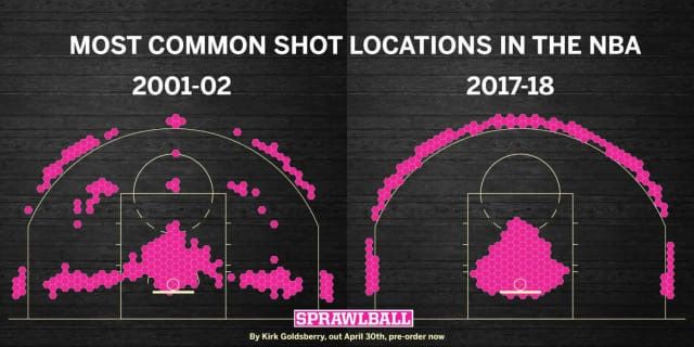
Abstract

Technology has revolutionized many industries and sport is no exception, looking for ways to
improve your team, taking advantage of any resource.
The goal of data analysis is to find a solution to the questions we ask ourselves. So far, coaches
have relied solely on intuition, but data is an opportunity to move away from cognitive biases
and get closer to reality.
This work is done in the context of a basketball team that competes in the Euroleague and asks
what type of players it should have to maximize its chances of becoming champion. To be able
to do this, player data from the last 5 years has been collected and ’clustering’ is performed,
which is a machine learning technique that groups the players who have similar characteristics.
Apart from this, this clustering has other applications like finding a similar substitute for a
player who is going to another team or to see an evolution from the five traditional positions in
basketball.

                                                                                                2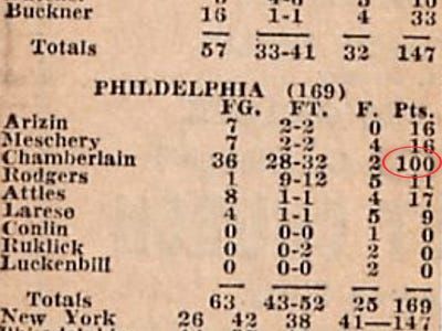
Resum

La tecnologia ha revolucionat moltes indústries i l’esport no és cap excepció, buscant constan-
ment maneres de fer millorar al teu equip, aprofitant qualsevol recurs.
La intenció de l’anàlisi de dades es trobar solució a preguntes que ens realitzem. Fins ara, s’ha
confiat únicament amb la intuició, però les dades són una oportunitat per allunyar-se dels biaixos
cognitius i apropar-se a la realitat.
Aquest treball es realitza en el context d’un equip de bàsquet que competeix a la Eurolliga
i es pregunta quina tipologia de jugadors ha de tenir per maximitzar les seves possibilitats
d’esdevenir campió. Per poder-ho dur a terme, es recopilen les dades dels jugadors dels últims
5 anys i es realitza ’clustering’, una tècnica de machine learning que agrupa els jugadors que
tenen caracterı́stiques semblants.
A part d’això, el clustering té altres aplicacions com trobar un substitut semblant d’un jugador
que marxa a un altre equip o veure l’evolució de les tradicionals cinc posicions del bàsquet.

                                                                                                    3
Resumen

La tecnologı́a ha revolucionado muchas industrias y el deporte no es una excepción, buscando
constantemente maneras de hacer mejorar a tu equipo, aprovechando cualquier recurso.
La intención del análisis de datos es encontrar solución a preguntas que nos realizamos. Hasta
ahora, se ha confiado únicamente en la intuición, pero los datos son una oportunidad de alejarse
de los sesgos cognitivos y acercarse a la realidad.
Este trabajo se realiza en el contexto de un equipo de baloncesto que compite en la Euroliga y se
pregunta qué tipologı́a de jugadores debe tener para maximizar sus posibilidades de convertirse
en campeón. Para poderlo llevar a cabo, se recopilan los datos de los jugadores de los últimos 5
años y se realiza ’clustering’, una técnica de Machine Learning que agrupa a los jugadores que
tienen caracterı́sticas similares.
A parte de esto, el clustering tiene otras aplicaciones como encontrar un sustituto parecido a
un jugador que se va a otro equipo o ver la evolución de las tradicionales cinco posiciones en
baloncesto.

                                                                                                4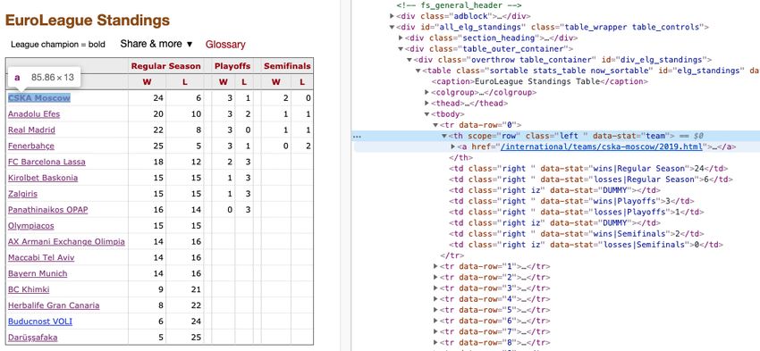
Acknowledgements

Firstly, I would like to thank my thesis advisor Prof. Josep Ramon Morros for the weekly feed-
back and the predisposition. Every time I have had any doubt he has given me great advice to
keep going.

Special thanks to Adrià Arbués who has been a mentor to me since I started with Basketball
Analytics, has also helped during the project, and has contributed with a lot of free resources to
the basketball community.

I would also like to thank Fran Camba, whose work has boosted my curiosity in player clus-
tering, and Nacho Gámez for his contribution with the scraping of play-by-play and shot chart
scraped Euroleague data.

I want to thank the Sports Analytics community to share their knowledge online and especially,
the ones who participated in the talks I chaired.

                                                                                                5
Contents
Abstract                                                                                                                                                   2

Resum                                                                                                                                                      3

Resumen                                                                                                                                                    4

Acknowledgements                                                                                                                                            5

Contents                                                                                                                                                   7

List of Figures                                                                                                                                            8

List of Tables                                                                                                                                             9

1   Introduction                                                                                                                                           10
    1.1 Statement of purpose . . . . . .               .   .   .   .   .   .   .   .   .   .   .   .   .   .   .   .   .   .   .   .   .   .   .   .   .   11
    1.2 Requirements and specifications                .   .   .   .   .   .   .   .   .   .   .   .   .   .   .   .   .   .   .   .   .   .   .   .   .   12
    1.3 Methods and procedures . . . .                 .   .   .   .   .   .   .   .   .   .   .   .   .   .   .   .   .   .   .   .   .   .   .   .   .   12
    1.4 Work plan . . . . . . . . . . . .              .   .   .   .   .   .   .   .   .   .   .   .   .   .   .   .   .   .   .   .   .   .   .   .   .   12

2   State of the art                                                                                                                                       14
    2.1 Sports Analytics . . . .   .   .   .   .   .   .   .   .   .   .   .   .   .   .   .   .   .   .   .   .   .   .   .   .   .   .   .   .   .   .   14
    2.2 Basketball Analytics .     .   .   .   .   .   .   .   .   .   .   .   .   .   .   .   .   .   .   .   .   .   .   .   .   .   .   .   .   .   .   15
          2.2.1 Box score . . .    .   .   .   .   .   .   .   .   .   .   .   .   .   .   .   .   .   .   .   .   .   .   .   .   .   .   .   .   .   .   15
          2.2.2 Play-by-play .     .   .   .   .   .   .   .   .   .   .   .   .   .   .   .   .   .   .   .   .   .   .   .   .   .   .   .   .   .   .   17
          2.2.3 Player tracking    .   .   .   .   .   .   .   .   .   .   .   .   .   .   .   .   .   .   .   .   .   .   .   .   .   .   .   .   .   .   18
    2.3 Machine Learning . . .     .   .   .   .   .   .   .   .   .   .   .   .   .   .   .   .   .   .   .   .   .   .   .   .   .   .   .   .   .   .   19
    2.4 Player Clustering . . .    .   .   .   .   .   .   .   .   .   .   .   .   .   .   .   .   .   .   .   .   .   .   .   .   .   .   .   .   .   .   20

3   Methodology/project development                                                                                                                        22
    3.1 Data collection . . . . . . . .            .   .   .   .   .   .   .   .   .   .   .   .   .   .   .   .   .   .   .   .   .   .   .   .   .   .   22
        3.1.1 Extraction . . . . . . .             .   .   .   .   .   .   .   .   .   .   .   .   .   .   .   .   .   .   .   .   .   .   .   .   .   .   22
        3.1.2 Transformation . . . .               .   .   .   .   .   .   .   .   .   .   .   .   .   .   .   .   .   .   .   .   .   .   .   .   .   .   23
        3.1.3 Loading . . . . . . . .              .   .   .   .   .   .   .   .   .   .   .   .   .   .   .   .   .   .   .   .   .   .   .   .   .   .   29
    3.2 Web Scraping . . . . . . . . .             .   .   .   .   .   .   .   .   .   .   .   .   .   .   .   .   .   .   .   .   .   .   .   .   .   .   29
    3.3 Data Cleaning . . . . . . . . .            .   .   .   .   .   .   .   .   .   .   .   .   .   .   .   .   .   .   .   .   .   .   .   .   .   .   30
    3.4 Clustering . . . . . . . . . . .           .   .   .   .   .   .   .   .   .   .   .   .   .   .   .   .   .   .   .   .   .   .   .   .   .   .   31
    3.5 Visualization . . . . . . . . .            .   .   .   .   .   .   .   .   .   .   .   .   .   .   .   .   .   .   .   .   .   .   .   .   .   .   31

4   Results                                                                                                                                                34

5   Budget                                                                                                                                                 38

6   Conclusions and future development                                                                                                                     39
    6.1 Conclusions . . . . . . . . . . . . . . . . . . . . . . . . . . . . . . . . . . . .                                                                39
    6.2 Future work . . . . . . . . . . . . . . . . . . . . . . . . . . . . . . . . . . . .                                                                40

                                                                                                                                                           6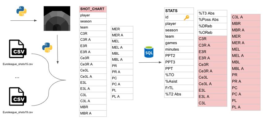
References   41

             7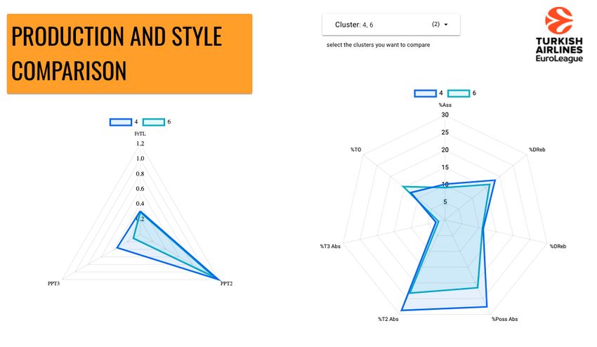
List of Figures
  1    Old box score from the Wilt Chamberlain’s 100 point game in 1962. . . . . . .            10
  2    Final Gantt chart . . . . . . . . . . . . . . . . . . . . . . . . . . . . . . . . .      13
  3    Barcelona’s box score of the game against Alba Berlin . . . . . . . . . . . . .          16
  4    Graphic from the book SprawBall by Kirk Goldsberry . . . . . . . . . . . . . .           16
  5    Play-by-play of a CSKA Moskow-Olympiacos Piraeus game . . . . . . . . . .                18
  6    Player tracking of a Clippers-Rockets game . . . . . . . . . . . . . . . . . . .         19
  7    Graphic with the 23 offensive roles by the frequency of type of play . . . . . .         20
  8    Reference system for mapping shots in “Shooting tetradecagons” by Adrià Arbués         21
  9    Example of a complete shot chart of a game . . . . . . . . . . . . . . . . . . .         23
  10   Information about Alex Abrines from Euroleague’s website . . . . . . . . . . .           23
  11   Final table showing the source of every parameter . . . . . . . . . . . . . . . .        24
  12   Box score’s contribution to the stats table . . . . . . . . . . . . . . . . . . . .      24
  13   Play-by-play’s contribution to the stats table . . . . . . . . . . . . . . . . . . .     26
  14   Shot regions . . . . . . . . . . . . . . . . . . . . . . . . . . . . . . . . . . . .     28
  15   Shot regions . . . . . . . . . . . . . . . . . . . . . . . . . . . . . . . . . . . .     29
  16   HTML code of Basketball Reference website . . . . . . . . . . . . . . . . . .            30
  17   First steps for Web Scraping . . . . . . . . . . . . . . . . . . . . . . . . . . .       30
  18   Clusters overview page . . . . . . . . . . . . . . . . . . . . . . . . . . . . . .       32
  19   Production and style comparison for clusters 4 and 6 . . . . . . . . . . . . . .         33
  20   Clusters of the last 3 Euroleague champions . . . . . . . . . . . . . . . . . . .        37
  21   Jobs in the data field and its characteristics . . . . . . . . . . . . . . . . . . . .   39

                                                                                                8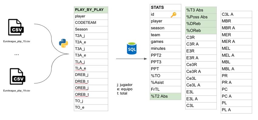
List of Tables
  1   Simple efficiency example .      .   .   .   .   .   .   .   .   .   .   .   .   .   .   .   .   .   .   .   .   .   .   .   .   .   .   .   17
  2   Shot regions achronim guide      .   .   .   .   .   .   .   .   .   .   .   .   .   .   .   .   .   .   .   .   .   .   .   .   .   .   .   28
  3   Results player clustering . .    .   .   .   .   .   .   .   .   .   .   .   .   .   .   .   .   .   .   .   .   .   .   .   .   .   .   .   34
  4   Luka Doncic’s evolution . .      .   .   .   .   .   .   .   .   .   .   .   .   .   .   .   .   .   .   .   .   .   .   .   .   .   .   .   36
  5   Costs of the project . . . . .   .   .   .   .   .   .   .   .   .   .   .   .   .   .   .   .   .   .   .   .   .   .   .   .   .   .   .   38

                                                                                                                                                   9
1 Introduction
So far, teams have relied on the experience and intuition of the coaching staff, but something
new has emerged, Data Analytics can be used to make better decisions. It can reveal trends and
metrics that can be used to increase the efficiency of your team.
When a basketball coach watches a game, he/she tries to analyze the strengths and weaknesses
of a team. Here is an example: it can happen that, one player scores 20 points, the conclusion
may be that this player is the best scorer of the team. But after that, a stat shows up saying that
it is his career-high and this season, he is only averaging 2 points a game, so the conclusion
that this player was the best scorer would have been wrong. As Ben Falk said in the Thinking
Basketball podcast [1], ”A human can watch and analyze a game better than data will ever be
able to, but data can analyze all games”.
We have available data for a long time ago (see Figure 1). In the beginning, points and fouls
were only captured in the box score 1 , but as time has gone by, we have much more.
Figure 1: Old box score from the Wilt Chamberlain’s 100 point game in 1962.
In the United States, they have evolved a lot from the box score, having tracking data and a
team of professionals helping the coaching staff. In Europe, Sports Analytics is starting but
some teams are already applying it.
This is why during the 2020 lockdown due to COVID-19, I started an initiative of Basketball
Analytics talks with experts on the field to learn how they apply this science to their teams.
Part 1 [2]
1A box score is a structured summary of the results from a sports competition
10• Fran Camba: how to characterize a player numerically to then cluster
• Jorge Lorenzo: draw tactical conclusions during the game in a professional team
• Sergi Oliva: from the origin of boxscore to player tracking, taking control of your own
analysis
Part 2 [3]
• Adrià Arbués: what is clustering and how to apply it
• Luis Clausı́n: how data can reduce the impact of cognitive biases on decision making
• Jesús Mayoral: the use of advanced statistics to sign players
Part 3 [4]
• Lluı́s Riera: Euroleague analysis to prepare for the season
• Rafael Jiménez: statistics in the ”minicopa” + analysis with FEB data
• Vı́ctor Solanes: Application of the 4 Factors from Dean Oliver in a u18 team
These talks, and especially the ones from Fran and Adrià were a starting point for this project.
They talked about clustering, which is an unsupervised Machine Learning technique that groups
items with similar characteristics. So I decided to try this technique with player data from the
Euroleague, the top-tier European professional basketball club competition.
1.1 Statement of purpose
Every Summer some teams sign some top players that make the team a championship contender.
Sometimes these expectations end up being true, others not, triggering a disappointing season.
But, can Machine Learning help in the decision-making of signing players to improve their
chances of becoming champions?
This can be done by looking at the past seasons. We have taken the last 5 seasons played, from
the 14-15 to the 18-19, due to COVID-19 the 19-20 season had no champion. First, research has
to be done about what data is there available. Then, build a database with relevant player stats
for every season.
Once this is done, we can process to do the player clustering to analyze what type of players do
the last Euroleague champions have in common.
111.2 Requirements and specifications
Requirements
• Although we can not access to the official Euroleague’s database, the stats are published
online, so web scraping can be done to get them and be able to have our own database.
• Velocity in execution is not something essential, but something to keep in mind
• The results from the clustering have to be clear so that the analysis can be done properly
Specifications
• As this is a proof of concept, no specifications are needed
1.3 Methods and procedures
This project uses some work developed by other authors. The parts of extraction, transformation
and clustering have been done using Python 3.7.
Within Python the following libraries have been used:
• Pandas [5] 1.1.4 for data manipulation: slicing, filtering, indexing...
• BeautifulSoup [6] 4.9.3 for Web Scraping which is a technique to extract data from web-
sites.
• Scikit-learn [7] 0.24.0 that provides tools for predictive data analysis, in this project it has
been used for the clustering
• Numpy [8] 1.17.2 that adds support for large, multi-dimensional arrays and matrices.
Google Data Studio has been used to create a dashboard to visualize the results with interactive
graphics.
1.4 Work plan
The Gantt chart of the project was first created with the Project Proposal and Work Plan, but
the theme of the project was not clear yet, so the Gantt chart has ended up being completely
different.
In the following weeks, the project was defined and with the Project Critical Review, a much
better Gantt chart was created.
This last chart has been followed pretty well, but there was a minor setback because I did not
consider a week or two to clean the data, which I would talk about in Chapter 3.
12This has been the final Gantt chart (Figure 2):
Figure 2: Final Gantt chart
132 State of the art
2.1 Sports Analytics
It is difficult to know when Sports Analytics was born, but the book, and later movie, ”Mon-
eyball” [9] made this science known with the story based on real events of how the Oakland
Athletics, a low-budget baseball team, used sabermetrics2 to prioritize personnel decisions in
professional sports. Billy Beane, the General Manager, signed players that fit his system. He
was very criticized but he was successful, and he revolutionized baseball’s modern era, and
now every major professional sports team in the US has an analytic expert or even an analytics
department.
Why is Sports Analytics useful?
Luis Clausı́n, in one of the talks I chaired, explains the work of Michael Lewis in his book
”The Undoing Project”[10]. He talks about these emotional influences and patterns that make
us unable to properly interpret the information we receive, called cognitive biases. The book
talks about the research of Daniel Kahneman and Amos Tversky[11], they studied the fact that
when we face a decision, like making a player play or not, we tend to fall on mental heuristics,
which are mental shortcuts that we use to make quick intuitive decisions, and may lead to
misjudgments.
Then, biases are the result of judgmental heuristics. Some types of heuristics are:
• Availability Heuristic: The most accepted, recent, or readily available information and
data are selected with priority by our brain.
• Affect Heuristic: The reliance on a “good” or “bad” feeling in making a decision. Basi-
cally, trusting your intuition to make quick judgment calls.
• Representative Heuristic: The use of stereotypes to judge the likelihood that something
belongs to certain group.
Some types of biases:
• Confirmation Bias: The tendency to favor, seek, interpret, and remember information
that confirms one’s beliefs or hypotheses.
• Overconfidence Bias: The overestimation of the confidence with which we trust our own
decisions or positions
• Novelty Bias: The tendency to prefer something just because it is new.
2 the application of statistical analysis to baseball records, especially to evaluate and compare the performance
of individual players.
14Heuristics and cognitive biases are mental limits [12]. Apart from that, we have time and re-
source limits. Many front office decision-makers do not have the time or resources to watch all
the games from all the candidates when signing a player.
Sports analytics is useful because it gives you more information with less time and, as stats are
numbers without emotions, they can prevent us from falling back to cognitive biases. Some real
use cases are:
• Opponent team and player analysis
• Team performance analysis
• Sports science: physical performance and medical decision-making
• Fan insights and engagement analysis
• Revenue optimization
• Real time decisions.
2.2 Basketball Analytics
In 2003, Basketball On Paper - Rules and Tools for Performance Analysis [13] was published,
it is considered the basic book for anyone who wants to start in the world of advanced statistics.
Some of the metrics used by the writer, Dean Oliver, are still used now.
To do any analysis, we first need data, more data means more information (unless we have
useless data). Basketball Analytics has evolved as different and more completed data sources
have been available: [14]
2.2.1 Box score
A box score is a structured summary of some stats collected during the game. Traditionally, it
contains the minutes played, made and missed shots, rebounds, assists, steals, blocks, turnovers
and fouls (see Figure 3).
It represents 24 rows of data per game approx., one row per player, and team totals. It requires
no processing. But the problem is that there is no context provided and it is purely based on the
outcome, meaning it can not be known how these things that are in there occurred.
Even with this basic form of data that had been in the industry for a lot of years, there have been
many changes in the last 20 years because people tried to figure out smarter ways to use it to
affect some change in the sport.
Maybe the most relevant of them, the change that has been the biggest attributed to analytics is
15Figure 3: Barcelona’s box score of the game against Alba Berlin
the rise of the 3-point shot. Nowadays, teams shoot a lot more threes than they used to.
Analysts realized that 3 is bigger than 2, which is obvious, by a significant 50% margin, so
instead of taking a long 2-point shot, it is better to step back and shoot a 3-pointer. In Figure 4
we see this change reflected:
Figure 4: Graphic from the book SprawBall by Kirk Goldsberry
Looking at rebounding numbers, coincidentally, the days that the team played the worst, the
players would rebound (on offense) the best. Another realization was that if there are more
misses because the team is not playing well, there are more opportunities to rebound the ball
and then players will rebound the ball more. So the great second revolution was that instead
16of looking at totals it is better to look at percentages, to be aware of opportunities. See the
example in Table 1.
Player Shots made Shots taken %
A 5 20 20%
B 4 5 80%
Table 1: Simple efficiency example
Although player A has scored more points, he has taken way more shots (more opportunities)
than B, so player B has been more efficient than player A.
These two realizations made this started being called Advanced Analytics.
From the box score, the concept of possessions was born. A team has the possession when they
are playing offense. The formula to calculate it is:
Possessions = 0.96 × [(Field Goal Attempts) + (Turnovers)+
0.44 × (Free T hrow Attempts) − (O f f ensive Rebounds)]
One of the things that was a challenge with the box score data source is that context matters.
Rebounding is not the same against smaller and lazy opponents than against taller and active
opponents.
Advanced Analytics opened the door to some people from different disciplines getting into
basketball teams and being able to keep improving.
2.2.2 Play-by-play
A play-by-play is defined as reporting on every action as it occurs on the game chronologically
(see Figure 5).
The data is still outcome-based and it is not so much data, just 400 rows of data per game which
are the number of events that happen. But there is some context in terms of knowing who is
on the court when an event happens, which was the score, the time left... so we can understand
better.
With this information, we can do lineup optimization: understanding which groups of players
play better together, which are the players we have on the court when we are effective. Also, be
able to identify if two players perform well together.
17Figure 5: Play-by-play of a CSKA Moskow-Olympiacos Piraeus game
Another advancement was about all those things that coaches call intangibles, meaning things
that do not get reflected in the stat sheet because technically the player is not responsible for the
outcome, but he/she has helped to make this happen.
With this, we can start looking at, not only how many rebounds the player gets or what defensive
rebound percentage the player has, but also what happens when this player is on the court. So
maybe his effect is not by getting the ball but by making his teammates get the ball.
The challenge with play-by-play data is that we know the what and when in terms of context,
but we do not know the how or the why. We still do not know the process that led to something
happening.
2.2.3 Player tracking
Tracking is a technology able to identify every player (and the ball) on the court at every moment
through video (Figure 6). Currently, it is only used in the NBA, this is why it is considered the
most advanced basketball league in Analytics.
From tracking data, analysts receive large files that give essentially x, y, and z positions of
every player at 25 frames per second rate. That equates to a million rows of data per game, so
the available data has increased exponentially, and so the techniques that they have to use.
With this huge dataset of just positions, they can figure out what actions and what type of
situations are happening in the game: what is a pass, a dribble, a particular play a team is
running, and other tactical situations. This provides rich contextual information and it is not
only based on the outcome but also what route the player took to get to that outcome and even
where were the other players and how were they moving when it happened.
18Figure 6: Player tracking of a Clippers-Rockets game
Knowing the context allows analysts to have a conversation with coaches in a sense that apart
from identifying the problem, they can provide tools to find the solution. For example, when
not finding a particular important shot in the game, being able to identify which situations have
led to that, which situation has not led to that but we are okay with, or which situations we are
not taking advantage of that could lead to that.
The available jobs in basketball nowadays have changed significantly because knowing how to
do Machine Learning techniques over this dataset is required.
The most interesting advance is being able to quantify and analyze trade-offs. Basketball is
a game of trade-offs, coaches make a bet on what they are trying to do, strengthening one
part of the game by probably weakening another part. For example, defensively in a particular
situation, what is better for the team, to put two defenders to cover the ball or isolate the player
in a 1-on-1?
2.3 Machine Learning
Second Spectrum is the Official Tracking Provider for the NBA, among other leagues, not only
they have developed the software to get files with the position of the players in the court, but
also they have implemented ML algorithms to get insights.
As Rajiv Maheswaran, the CEO and Co-Founder of Second Spectrum explained in his TED talk
[15], they implemented classification to identify tactical situations that occur in basketball, for
example, a pick and roll3 . Classification is a supervised learning technique that after introducing
3 offensive play in which a player sets a screen for a teammate with the ball and then moves toward the basket
19labeled data from previous games, like these files but with the added information of what is a
pick and roll and what is not, can identify what is a pick and roll and what is not for future
games. This is called spatiotemporal pattern recognition.
With spatiotemporal pattern recognition, they are also able to quantify how good or how bad a
shot is by looking at every shot taken and its situation: where the shot is, what is the angle to the
basket, where are the defenders standing, which shot type it is, and more. With this information,
they build a model that predicts what is the likelihood that this shot would go in under these
circumstances. They can know the quality of the shot and the quality of the shooter.
2.4 Player Clustering
There have been other projects which have used clustering. Todd Whitehead used [16] the NBA
play-type data4 from the 17-18 season to define 23 different offensive roles and created a few
Tableau dashboards to describe the groups that were formed (see Figure 7). His goal was to see
how basketball has evolved from the classic five positions.
Figure 7: Graphic with the 23 offensive roles by the frequency of type of play
4 The NBA’s individual play-type data are provided by Synergy using a proprietary, real-time, video-indexing,
statistical engine that logs every play of every game.
20Samuel Kalman and Jonathan Bosch presented this work [17] in the MIT Sloan Sports Analytics
Conference. One of the goals is the same as the project before but with the addition that it also
provides insight into which combination of player types yield the most effective basketball
performance. They used box score and play-by-play data from ten NBA seasons (2009-2018).
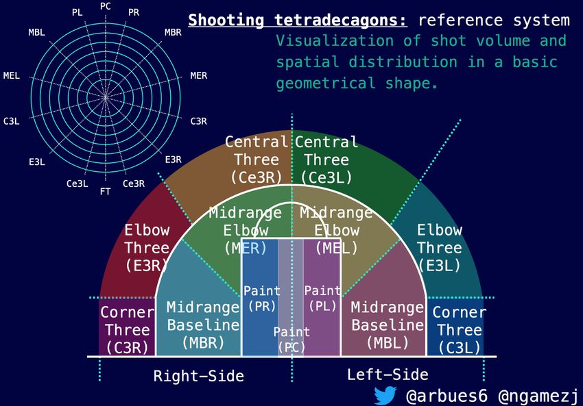
Adrià Arbués [18], used Euroleague data focusing on shooting with the goal of, through clus-
tering, being able to spot different types of group players.
This was done by splitting the court in 14 regions (see Figure 8, and then seeing how players
perform at each zone by mapping it in tetradecagons (14 side polygon), where all the vertices’
orientation correspond to a different type of spatial shot.
Figure 8: Reference system for mapping shots in “Shooting tetradecagons” by Adrià Arbués
213 Methodology/project development
Note: The code is available on GitHub: github.com/dmolins/euroleague-clustering
3.1 Data collection
In every analysis, we need data. Sometimes data is provided and other times techniques have to
be used to take this data. Because of this, an ETL (Extraction, Transformation and Loading of
the data) process has been followed.
3.1.1 Extraction
In order to do a consistent analysis, data from 4 different resources will be gathered: box score,
play-by-play, shot chart, and player info.
1. Box score
In this case Web Scraping has been used to take the data from Basketball Reference [19],
which is a very popular and reliable website where we can find these stats averaged for
every player during the whole season.Web Scraping refers to the extraction of data from a
website. This information is collected and then exported into a format that is more useful
for the user. We do it using Python and export the data into CSV files.
2. Play-by-play
The play-by-play data gives us more information. In this case, thanks to Nacho Gámez,
we already have CSV files that have been built from the Euroleague website [20].
3. Shot chart
It is another data source that gives information about the shots made or miss by every
player and its position on the floor (see Figure 9). Like the play-by-play data, thanks to
Nacho Gámez’s work, we already have the CSV files.
22Figure 9: Example of a complete shot chart of a game
4. Player info
The resources mentioned give us information about the games, but we also need informa-
tion about the players: height, nationality, age and position (see Figure 10). We can access
this information also on the Euroleague website, which has been scraped.
Figure 10: Information about Alex Abrines from Euroleague’s website
3.1.2 Transformation
The goal is to take relevant data to do the clustering, so this phase consists of transforming the
data extracted into relevant and structured data for the analysis.
To explain it, it is better to start from the end. In Figure 11 we can see the table used to cluster
the players, a fact table called stats, which contains information from games (box score, play-
by-play, and shot chart). The player info table has not been used but it has been taken in case it
is needed in the future.
With the stats collected in the stats table we have information about the player’s role, his scoring
efficiency, how many possessions he finishes when he is on the court, his playing style and his
23Figure 11: Final table showing the source of every parameter
shooting preferences. The meaning of every stat, every parameter for the clustering, will be
explained below.
But to arrive here, previously some transformations have to be done.
1. Box score
Directly from the CSV files obtained, the box score table (Figure 12) is built.
Figure 12: Box score’s contribution to the stats table
24To get the stats that we want, we use the following formulas:
Games played:
games = G
Minutes per game:
minutes = MP
The points the player added per 2 point shot attempted:
2 × 2P
PPT 2 =
2PA
The points the player added per 3 point shot attempted:
3 × 3P
PPT 2 =
3PA
The points the player added per shot attempted, taking into account 2 and 3-pointers:
2 × 2P + 3 × 3P
PPT =
FGA
Turnover rate, meaning the percentage of the possessions the player finishes that end up
with a turnover:
T OV × 100
%T O =
FGA + FTA × 0.44 + AST + T OV
Assist rate, same concept for assists:
AST × 100
%Asist =
FGA + FTA × 0.44 + AST + T OV
Frequency of free throw shooting, meaning how many free throws the player scores com-
pared to his/her field goals attempts:
FT
FrT L =
FGA
2. Play-by-play
For the play-by-play data we previously have to process the data that we get from the
CSV files, these are the most relevant columns the files have:
• Codeteam → (p.e: BAR for FC Barcelona)
• Player → who did the action
25• Playinfo → type of play (Two Pointer, Defensive Rebound, Foul, Substitution...)
• Game → game identifier
From this data source, information about the usage of a player will be obtained by how
many of each stat the player had ( j) and how many the team had when the player was on
the court ( e). The stats that represent usage are shots attempted(2 and 3-pointers, T2A
and T3A), free throw shooting (TL) and turnovers (TO).
Apart from this, rebounding ability is also measured by summing up the rebounds, de-
fensively and offensively, a player had ( j) and the available rebounds the player he could
have got when he was on the court ( t).
Figure 13: Play-by-play’s contribution to the stats table
With these stats, the play by play table can be built, and from it we can get the stats that
are going to be used in the clustering (see Figure 13):
The percentage of two-point shots absorbed, meaning the percentage of two-point shots
a player took out of ones the team took when he was on the court:
T 2A j × 100
%T 2Abs =
T 2Ae
The percentage of three-point shots absorbed, same concept for 3 point shots:
T 3A j × 100
%T 3Abs =
T 3Ae
The percentage of possessions absorbed, same concept for possessions:
26(T 2A j + T 3A j + T LA j × 0.44 + T O j − OREB j ) × 100
%PossAbs =
T 2Ae + T 3Ae + T LAe × 0.44 + T Oe − OREBt
The percentage of defensive rebound, the defensive rebounds the player took out of the
total he could have got:
DREB j × 100
%DReb =
DREBt
The percentage of offensive rebound, same concept for the offensive ones:
OREB j × 100
%OReb =
OREBt
3. Shot chart
This one is more tricky. The CSV files give information of every shot taken with:
• The player who took the shot
• Type of shot: two/three-pointer made/missed or free throw
• The points added with the shot (0, 1, 2 or 3)
• The position of the shot, with coordinates (in cm) on the x (COORD X) and y-axis
(COORD Y)
For the coordinates, the origin is under the rim, and as you go further, COORD Y in-
creases. Shots taken from the left (as if you see it from the court) have COORD X > 0,
and from the right, < 0.
Although the files give a shot zone, I think this can be improved, so an image has been
created with other regions defined very close to the one Adrià Arbués created [21].
The image in Figure 14a is a representation done with Photoshop from the created image
Figure 14b, which has been created with Python to be extremely precise. The grey-scale
image has been created superposing polygons so that each zone in this image has a unique
label.
Every shot region has an acronym, following the guide in table 2:
27(a) With shot region names (b) Grey-scale
Figure 14: Shot regions
Digit Meaning Digit Meaning Digit Meaning
3 3-pointer C Corner R Right
M mid-range E Elbow L Left
P paint Ce Central C Central
B Base-line
Table 2: Shot regions achronim guide
To know the shots made and attempted per game for every player and every shot region,
a Python script has been created that goes shot by shot identifying the region and adding
it to the player who took it. The process is as follows: first, the coordinates (x,y) are
converted from cm to pixels in the image (X,Y). Then, as all the pixels of a given region
of the image have the same label, it is possible to know the region from where the shot was
thrown by simply taking the value of the pixel at position (X,Y). With this information,
the shot chart table is built as shown in Figure 15:
28Figure 15: Shot regions
So for example, MBR stands for the made shots in the Mid-range Baseline Right region,
and MBR A for the attempted shots in the same region.
4. Player info
No transformation is required for player information, just importing it to an SQL table.
3.1.3 Loading
SQL has been used to join the box score, play by play, and shot chart tables into a view, which
has been stored in a local server.
3.2 Web Scraping
Web Scraping has been used to extract the box scores and player info from websites, so in this
chapter, the process will be briefly explained.
First, the data source has to be inspected to be able to understand, through the HTML code,
how the web is structured. In Figure 16 we see the Basketball-Reference page for the 18-19
Euroleague season, we can see that the links for every team who competed that season are
stored in a table (table class=”sortable stats table now sortable” id=”elg standings” data-cols-
to-freeze=”1”).
A connection has to be made with the website that wants to be scraped and then parse the HTML
29Figure 16: HTML code of Basketball Reference website
page into a container using Beautiful Soup, as can be seen in Figure 17.
Figure 17: First steps for Web Scraping
After that, you have to go directly to the information you want to get using functions like find
or find all taking as a parameter the element where the information is. Figure 17, shows that
every team is stored inside a row of the table (tr).
Once we have the information we want, it is stored in a DataFrame using the pandas’ library
that allows us, when it is finished, to export the data into a CSV file.
3.3 Data Cleaning
Cleaning the data is essential to get at least acceptable results. After gathering all the data, there
was a complete revision to assure that the data did not have any mistakes. Some mistakes were
30found and made me step back to correct them. The origin of these mistakes can be found in the
ETL process or even in the data sources.
A remarkable bug that was found was that there were some cases that the values obtained were
not being coherent and it was because of the collected data from the Euroleague website. It was
found that there were cases that the same player was named differently in different games. For
example, for some games, we had stats from Alex Abrines and for other games, from Alejandro
Abrines, so this was interpreted as two different players. As a solution, both ”players” were
summed up and saved with the name of Alex Abrines.
3.4 Clustering
Once we have the data structured and cleaned, we can proceed to do the clustering. Python and
the Scikit-learn library have been used. First, the connection with the SQL server is done to get
the stats table, and the parameters that are going to be used are introduced into a NumPy matrix.
The algorithm used to do the clustering has been the K-means algorithm [22]. K-means clusters
data by trying to separate samples in n groups of equal variance. It requires the number of
clusters to be specified.
After trying with a different number of clusters, the results were not being adequate.
It was observed that players were falling into clusters that they did not fit. What these players
had in common was that they played for very few minutes. As a solution, the query was filtered
by the players that played more than 5 minutes per game because those who did not, their stats
were not reliable for being a very small sample that introduces noise. There were also removed
those players who played less than five games.
K-means clustering is ”isotropic” in all directions of space [23] and therefore tends to produce
more or less round (rather than elongated) clusters. In this situation, leaving variances unequal is
equivalent to putting more weight on variables with smaller variances. This is why standardizing
the parameters before clustering was tried.
These two adjustments made improve the results and, after testing the clustering with a different
number of clusters, the best results have been fixing this value to 10.
3.5 Visualization
To interpret the results, visualizing them with graphics can help. The program Google Data
Studio has been used to do so, seeing the difference between clusters and understanding what
characteristics does a player need to have to be in a particular cluster. The dashboard created is
available for anyone to see it and be able to interact with it:
https://datastudio.google.com/s/j1yrSOAvW0Y
31Here are some of the used graphics:
Figure 18: Clusters overview page
In Figure 18 there is an overview of all the clusters that allow us to see the main difference
between them. If it is not very clear what distinguished two specific clusters, on another page,
there is the possibility to see it with more detail. For example, in Figure 19 we use this page to
compare clusters 4 and 6:
32Figure 19: Production and style comparison for clusters 4 and 6
334 Results
The results from the clustering have finally been satisfactory, with 10 differentiated groups. To
understand the results (see Table 3), basketball knowledge is required.
ID Cluster name Characteristics Some players
0 Secondaries few minutes, low %Poss, high %Ass Balbay, Vezenkov, young-
sters
1 3-point spot-up for- high 3 pointers from corners, few paint shots, Datome, Micov, Thompkins
wards rebound
2 3-point specialists few minutes, high %T3 Abs, low in anything Mahnmoutoglu, Taylor,
else Bertrans
3 3&D low shooting volume but efficient, rebound Claver, Kurbanov, Kuzmin-
skas, Blazic
4 Top bigs high rebound, high volume paint shots, no 3FG Tomic, Shengelia, Vesely
5 Star exteriors very high %T3 Abs, especially above the Llull, Doncic, Spanoulis
break, high minutes, high usage
6 Second unit bigs low minutes and usage, high rebound, high Diop, Dorsey, Slaughter
%TO
7 Mid-range forwards high mid-range volume, low %Ass, low 3FG Printezis, Gentile, Jankunas
8 Second sword exteri- low %T2 Abs, high volume and efficiency in Carroll, Rudy, Abrines
ors 3FG
9 Ball-dominant High minutes, %Ass and %Poss, mid-range Calathes, Heurtel, De Colo
guards
Table 3: Results player clustering
0. Secondaries
In this group, there are players who play the least minutes and have a secondary role in
their teams. In the minutes they play, their first option is to play for the team, this is why
34they finish few possessions, and a lot of them end up with an assist to another teammate.
Young players in their first season are common to be here.
1. 3 point spot-up forwards
Here we have those players who can stretch the floor because of their efficient 3 point
shot, specially from the corners. In offense they are usually opened, this is why their
strength is not the offensive rebound.
2. 3 point specialists
It has been seen the importance of the 3 point shot in modern basketball, so there are
players who can make it to a top league with that being their only strength. They play few
minutes and they do what they know. Consequently, they do not dribble to the basket so
they do not score near the rim or receive fouls to get to the free throw line.
3. 3&Ds
3&D is a concept given for those players who can do a little bit of everything, we can find
players that can play in multiple traditional positions because of their versatility. They
have a low shooting volume but they are efficient. They also help in rebounding.
4. Top bigs
In this cluster we find those players who move close to the basket and they can score and
rebound a lot. They finish strong at the rim, this is why they are fouled a lot.
5. Star exteriors
In this group there are the type of players that usually receive more attention. They are
the most used in terms of minutes played and shooting volume. They shoot a lot of threes,
specially above the break (3 point shots that are not from the corners).
6. Second unit bigs
Similar to the top bigs cluster, but with the difference that these players shoot less and are
less efficient, so they are not as skilled as the other cluster. This also shows in the fact that
they turn the ball over a lot.
7. Mid-range shooters
Although these players can shoot from 3, their strength is the mid-range shot. As their
focus is on scoring, they give few assists.
8. Second sword exteriors
Players from this cluster are outside scorers who do not finish much in the paint and do
not play a lot of minutes but are key in terms of scoring from 3 and play-making.
9. Ball-dominant guards
35Here we find those players who dominate rhythm of the game. They can score from in-
side and outside, they use a lot the mid-range area, but their strength is assisting to other
teammates.
As ten clusters have been fixed, there is not a cluster with one of the traditional five positions
(point-guard, shooting-guard, small-forward, power-forward, and center), even if the number of
clusters is fixed to five, these traditional positions do no appear. On the other hand, it can be
seen that these new roles (better said than positions) focus more on the player’s production and
efficiency, although the bigs (clusters four and six) can be distinguished from others.
Furthermore, it is interesting to see that few players are in the same cluster for all of the five
seasons. This can be because they can develop or get older so their style and production changes,
also if a player changes from one team to another, he may play a different role there. In Table 4
there is the example of Luka Doncic’s evolution.
Season Cluster Info
15-16 Secondary First season in Euroleague with 16 years old
16-17 Second sword exterior He starts to play regularly being important for the team
He wins the MVP award5 and helps Madrid winning the
17-18 Exterior star
Euroleague. Next year he goes to the NBA
Table 4: Luka Doncic’s evolution
Once the clusters are done, can we see clusters on the last champions that other teams do not
have? Do these teams have a specific number of players of a specific cluster that other teams do
not? The champions from the last five seasons have been compared between each other and also
compared to the other teams. In Figure 20 there are graphics done with Google Data Studio that
show the number of players from each cluster of the last 3 Euroleague champions.
36Figure 20: Clusters of the last 3 Euroleague champions
We can conclude, only by watching Figure 20 that a championship team must have at least two
players from cluster 4 (Top bigs), one or more player from cluster 2 (3 point specialists), at least
one player from cluster 5 (exterior stars)... but many other teams who were not champions have
these type of players, so this clustering is not conclusive to define a team champion.
375 Budget
This project has lasted four months, so all of the costs will be estimated monthly and finally
multiplied by four.
All of the software used is Open Source and no raw materials have been used. The only material
used is the computer which is a MacBook Pro (13-inch, 2017, Two Thunderbolt 3 ports) that
had a price of 1500 C, taking into account that a computer can last 4 years, the cost for one
month is:
1500
Monthly PCCost = = 375EUR
4
The place to work has been a coworking space in Barcelona, where it is all included (WiFi,
lighting, printer, and more). This adds up a cost of 300 C monthly for a fixed desk. As it is close
to home and the talks I chaired were online, no transportation was needed.
Finally, wages. In this project, there has been a mentor as a Senior Engineer and me as a Junior
Engineer. The mentor has worked one hour per week for the weekly meetings with a salary of
60 C/hour and I have worked 20 hours per week for 10 C/hour. To get the cost from the salary, a
33% of social security benefits adds up.
Monthly Senior EngineerCost = (60 × 1 hour × 4 weeks) × 1.33 = 319.2EUR
Monthly Junior EngineerCost = (10 × 20 hour × 4 weeks) × 1.33 = 1064EUR
Then the costs for this project are (see Table 5):
Item Cost
Computer 375EUR
Senior Engineer 319.2 EUR
Junior Engineer 1064 EUR
Coworking space 300 EUR
Total (monthly) 2058.2EUR
TOTAL COST (4 months) 8232.8 EUR
Table 5: Costs of the project
386 Conclusions and future development
6.1 Conclusions
This project has involved all the parts of analysis, from the data extraction to the final intepreta-
tions. With it, it has allowed me to learn a little bit from every step of the process: what a Data
Engineer (ETL process and Data Cleaning), a Data Scientist (ML techniques, although they do
way more than that), and Data Analyst (visualization and final analysis) do. In Figure 21 these
jobs with more detail are shown.
Figure 21: Jobs in the data field and its characteristics
Although the results may not help to find the type of players that make a Euroleague team
champion, other applications have been found. When a player goes to another team or retires,
this can be helpful to find a replacement with similar skills so that the coach does not need to
change the way the team plays.
Another possible application could be to identify teams with similar players. So when a partic-
ular strategy has worked against one team, if we face another one with similar players, the same
strategy can work against them.
With this, it has also been proven that basketball has evolved and traditional positions are not
as defined as before. I do not think they do not exist anymore, because some clusters are very
related to these positions but it is true that new types of players can be found. This information
can help coaches boost their team’s performance by being aware of their players’ strengths and
weaknesses.
39Once this is coming to the end, now that I look behind I would have done some things differ-
ently. I did not expect the original data to have mistakes. Anyway, I should have planned to
invest time in analyzing it beforehand. So the two weeks I dedicated to clean the data would
probably have been less. Furthermore, the ’timing’ of each Work Package was not as I expected,
the project has made me understand that, more or less, it is 50% to get the data and structure it,
20% to clean it, 10% to apply clustering, and 20% to analyze the results.
Personally, I have enjoyed this project a lot, it has allowed me to put together my two passions:
basketball, which has been for a long time, and data, which is ”new” for me. This work has
made me realized that this is what I want to do in the future but this is just the beginning, so I
have to learn and experience a lot to arrive at that point.
6.2 Future work
Even though the results obtained are not enough to know which players a team needs to have
to become champion, it does not mean that it is impossible to know using clustering. I would
like to continue this project by trying other methods like K-means with a lot of clusters (more
than 20), applying PCA before clustering, or trying other algorithms like DBSCAN or Gaussian
mixture model. Also, with more data, a better analysis can be done. The same process can be
applied using play-type or tracking data, which hopefully, will be available in Europe soon.
It is said that the NBA is way more physical than in Europe, and the way is played is different,
so it would be interesting to do the same for other leagues and compare the resulting clusters.
Besides, some prospects from Europe decide to go to the NBA after playing in the Euroleague,
so another future work could be to analyze if they play the same way or also predict how well a
player from Europe could do in the NBA.
40References
[1] Thinking Basketball. The one-number debate, film in analytics measuring defense. URL:
https://open.spotify.com/episode/1OxP4p8zDa4fTldJJX8eV8?si=ihjzmaEzQVKKY9_
1HIzwnQ.
[2] David Molins Gracia. Charla de Estadı́stica Avanzada en Baloncesto - Parte 1. URL :
https://www.youtube.com/watch?v=eKZ8Ss29ibw&t=1240s.
[3] David Molins Gracia. Charla de Estadı́stica Avanzada en Baloncesto - Parte 2. URL :
https://www.youtube.com/watch?v=KHWPxl5i_j4&t=4641s.
[4] David Molins Gracia. Charla de Estadı́stica Avanzada en Baloncesto - Parte 3. URL :
https://www.youtube.com/watch?v=dJaALNv_NsY&t=2217s.
[5] The pandas development team. pandas-dev/pandas: Pandas. Version latest. Feb. 2020.
DOI : 10 . 5281 / zenodo . 3509134. URL : https : / / doi . org / 10 . 5281 / zenodo .
3509134.
[6] Leonard Richardson. “Beautiful soup documentation”. In: April (2007).
[7] F. Pedregosa et al. “Scikit-learn: Machine Learning in Python”. In: Journal of Machine
Learning Research 12 (2011), pp. 2825–2830.
[8] Charles R. Harris et al. “Array programming with NumPy”. In: Nature 585.7825 (Sept.
2020), pp. 357–362. DOI : 10.1038/s41586-020-2649-2. URL: https://doi.org/
10.1038/s41586-020-2649-2.
[9] Michael Lewis. Moneyball. The Art of Winning an Unfair Game. W. W. Norton Com-
pany, 2004.
41[10] Michael Lewis. The Undoing Project. A Friendship That Changed Our Minds. W. W.
Norton Company, 2016.
[11] Amos Tversky and Daniel Kahneman. “Judgment under Uncertainty: Heuristics and Bi-
ases”. In: American Association for the Advancement of Science 185.4157 (1974). DOI :
https://www.jstor.org/stable/1738360.
[12] Brendan Kent. Sports Analytics 101: The Case for Sports Analytics. URL : https : / /
brendankent.com/2020/10/08/sports-analytics-101-the-case-for-sports-
analytics/.
[13] Dean Oliver. Basketball on Paper. Rules and Tools for Performance Analysis. POTOMAC
BOOKS, 2004.
[14] Sergi Oliva. Sports and Analytics. URL: https://youtu.be/5FxvPGYxcBQ.
[15] Rajiv Maheswaran — TED Talks. The Math Behind Basketball’s Wildest Moves. URL:
https://www.youtube.com/watch?v=66ko_cWSHBU.
[16] Todd Whitehead. “Nylon Calculus: Defining 23 offensive roles using the NBA’s play-
type data”. In: fansided.com (2018). URL: https : / / fansided . com / 2018 / 10 / 15 /
nylon-calculus-defining-23-offensive-roles-nba-play-type-data/.
[17] Jonathan Bosch Samuel Kalman. “NBA Lineup Analysis on Clustered Player Tenden-
cies: A new approach to the positions of basketball modeling lineup efficiency of soft
lineup aggregates”. In: Mit Sloan Spors Analytics Conference (2020). URL: https://
uploads-ssl.webflow.com/5f1af76ed86d6771ad48324b/5f6a65517f9440891b8e35d0_
Kalman_NBA_Line_up_Analysis.pdf.
[18] Adrià Arbués. “Clustering Euroleague Shooters”. In: medium (2020). URL : https://
medium.com/@adria.arbues/clustering-euroleague-shooters-243f18d26c99.
42[19] Basketball Reference. URL: https://www.basketball-reference.com/international/
euroleague/.
[20] Official Euroleague Website. URL: https://www.euroleague.net/main/results.
[21] Adrià Arbués. Reference system for mapping shots in Shooting tetradecagons. URL :
https://miro.medium.com/max/700/1*zjG3TJq2qMHQwnnhjqN-QA.png.
[22] Scikit-learn. K-means. URL: https : / / scikit - learn . org / stable / modules /
clustering.html#k-means.
[23] stack overflow. Standarize before clustering. URL: https://datascience.stackexchange.
com/questions/6715/is-it-necessary-to-standardize-your-data-before-
clustering.
43You can also read