A generic multivariate framework for the integration of microbiome longitudinal studies with other data types - bioRxiv
←
→
Page content transcription
If your browser does not render page correctly, please read the page content below
bioRxiv preprint first posted online Mar. 24, 2019; doi: http://dx.doi.org/10.1101/585802. The copyright holder for this preprint
 (which was not peer-reviewed) is the author/funder, who has granted bioRxiv a license to display the preprint in perpetuity.
                                    All rights reserved. No reuse allowed without permission.

                 A generic multivariate framework for the integration of
                 microbiome longitudinal studies with other data types
                            Antoine Bodein 1† , Olivier Chapleur 2† , Arnaud Droit 1 , Kim-Anh Lê Cao 3,∗
                 1
                     CHU de Québec Research Center, Université Laval, Molecular Medicine department, Québec, QC, Canada,
                                     2
                                         Hydrosystems and Bioprocesses Research Unit, Irstea, Antony , France,
      3
          Melbourne Integrative Genomics, School of Mathematics and Statistics, University of Melbourne, Melbourne, VIC, Australia
                                                †
                                                    Both authors contributed equally to this manuscript

                                                            March 21, 2019

                                                                 Abstract
                 Simultaneous profiling of biospecimens using different technological platforms enables the study of
             many data types, encompassing microbial communities, omics and meta-omics as well as clinical or
             chemistry variables. Reduction in costs now enables longitudinal or time course studies on the same bi-
             ological material or system. The overall aim of such studies is to investigate relationships between these
             longitudinal measures in a holistic manner to further decipher the link between molecular mechanisms
             and microbial community structures, or host-microbiota interactions. However, analytical frameworks
             enabling an integrated analysis between microbial communities and other types of biological, clinical
             or phenotypic data are still at their infancy. The challenges include few time points that may be
             unevenly spaced and unmatched between different data types, a small number of unique individual
             biospecimens and high individual variability. Those challenges are further exacerbated by the inherent
             characteristics of microbial communities-derived data (e.g. sparsity, compositional).
             We propose a generic data-driven framework to integrate different types of longitudinal data measured
             on the same biological specimens with microbial communities data, and select key temporal features
             with strong associations at the sample group level. The framework ranges from filtering and modelling,
             to integration using smoothing splines and multivariate dimension reduction methods to address some
             of the analytical challenges of microbiome-derived data. We illustrate our framework on different types
             of multi-omics case studies in bioreactor experiments as well as human studies.

                 Keywords: Time course, data integration, splines, feature selection

    1        Introduction
    Microbial communities are highly dynamic biological systems that cannot be fully investigated in snapshot
    studies. The decreasing cost of DNA sequencing has enabled longitudinal and time-course studies to record
    the temporal variation of microbial communities (Faust et al., 2015; Knight et al., 2012). These studies
    can inform us about the stability and dynamics of microbial communities in response to perturbations or
    different conditions of the host or their habitat and can capture the dynamics of microbial interactions
    (Ridenhour et al., 2017; Bucci et al., 2016) or associate change of microbial features, such as taxonomies
    or genes, to a phenotypic group (Metwally et al., 2018).

        However, besides the inherent characteristics of microbiome data, including sparsity, compositionality
    (Aitchison, 1982; Gloor et al., 2017), its multivariate nature and high variability (Lê Cao et al., 2016b),
    longitudinal studies suffer from irregular sampling and subject drop-outs. Thus, appropriate modelling
    of the microbial profiles is required, for example by using splines modelling. Methods including loess
    (Shields-Cutler et al., 2018), smoothing spline ANOVA (Paulson et al., 2017), negative binomial smooth-
    ing splines (Metwally et al., 2018) or gaussian cubic splines (Luo et al., 2017) were proposed to model
          ∗ Corresponding   Author: kimanh.lecao@unimelb.edu.au

                                                                       1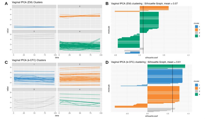
bioRxiv preprint first posted online Mar. 24, 2019; doi: http://dx.doi.org/10.1101/585802. The copyright holder for this preprint
 (which was not peer-reviewed) is the author/funder, who has granted bioRxiv a license to display the preprint in perpetuity.
                                    All rights reserved. No reuse allowed without permission.

    dynamics of microbial profiles across groups of samples or subjects. The aim of these approaches is to
    make statistical inferences about global changes of differential abundance across multiple phenotypes of
    interest, rather than at specific time points. These proposed methods are univariate, and as such, cannot
    infer ecological interactions (Morris et al., 2016). Other types of methods aim to cluster microbial profiles
    to posit hypotheses about symbiotic relationships, interaction or competition. For example Baksi et al.
    (2018) used a Jenson Shannon Divergence metric to visually compare metagenomic time series.

        Multivariate ordination methods can exploit the interaction between microorganisms, but need to be
    used with sparsity constraints, such as `1 regularization (Tibshirani, 1996), to reduce the number of vari-
    ables and improve interpretability through variable selection. Several sparse methods were proposed and
    applied to microbiome studies, such as sparse linear discriminant analysis (Clemmensen et al., 2011) and
    sparse Partial Least Squares Discriminant Analysis (sPLS-DA, Lê Cao et al. 2016a), but for a single time
    point. Therefore, further developments are needed to combine both time-course modelling with multivari-
    ate approaches to start exploring microbial interactions and dynamics.

        In addition, current statistical methods have mainly focused on a single microbiome dataset, rather
    than the combination of different layers of molecular information obtained with parallel multi-omics assays
    performed on the same biological samples. Data derived from each omics technique are typically studied
    in isolation, and disregard the correlation structure that may be present between the multiple data types.
    Hence, integrating these datasets enable us to adopt a holistic approach to elucidate patterns of taxo-
    nomic and functional changes in microbial communities across time. Some sparse multivariate methods
    have been proposed to integrate omics and microbiome datasets at a single time point and identify sets
    of features (multi-omics signatures) across multiple data types that are correlated with one another. For
    example, Gavin et al. (2018) used the DIABLO method (Singh et al., 2019) to integrate 16S, proteomics
    and metaproteomics in a type I diabetes study, Guidi et al. (2016) used sparse PLS (Lê Cao et al., 2008)
    to integrate environmental and metagenomic data from the Tara Oceans expedition to understand carbon
    export in oligotrophic oceans, and Fukuyama et al. (2017) used sparse Canonical Correlation Analysis
    (Witten et al., 2009) to integrate 16S and metagenomic data. However, methods or frameworks to in-
    tegrate multiple longitudinal datasets including microbiome data remain incomplete. To our knowledge,
    only one study (Ribicic et al., 2018) attempted to combine spline modelling (e.g. loess) with sparse Prin-
    cipal Component Analysis to explore the link between chemistry and microbial community data in the
    biodegradation of chemically dispersed oil, but their approach was not specifically looking for multi-omics
    signatures.

        We propose a computational approach to integrate microbiome data with multi-omics datasets in
    longitudinal studies. Our approach includes smoothing splines in a linear mixed model framework to model
    profiles across groups of samples, and builds on the ability of sparse multivariate ordination methods to
    identify correlated sets of variables across the data types, and across time. Our framework encompasses
    data pre-processing, modelling, data clustering and integration. It is highly flexible in handling one or
    several longitudinal studies with a small number of time points, to identify groups of taxa with similar
    behaviour over time, and posit novel hypothesis about symbiotic relationships, interactions or competitions
    in a given condition or environment, as we illustrate in two case studies.

    2      Method
    Our proposed approach includes pre-processing for microbiome data, spline modelisation within a linear
    mixed model framework, and a multivariate analysis for clustering and data integration (Figure 1).

    2.1      Pre-processing of microbiome data
    We assume the data are in raw count formats resulting from bioinformatics pipelines such as QIIME
    (Caporaso et al., 2010) or FROGS (Escudié et al., 2017) for 16S amplicon data. Here we consider the
    OTU taxonomy level, but other levels can be considered, as well as other types of microbiome-derived
    data, such as whole genome shotgun sequencing. The data processing step is described in Lê Cao et al.
    (2016a) and consists of:

                                                                       2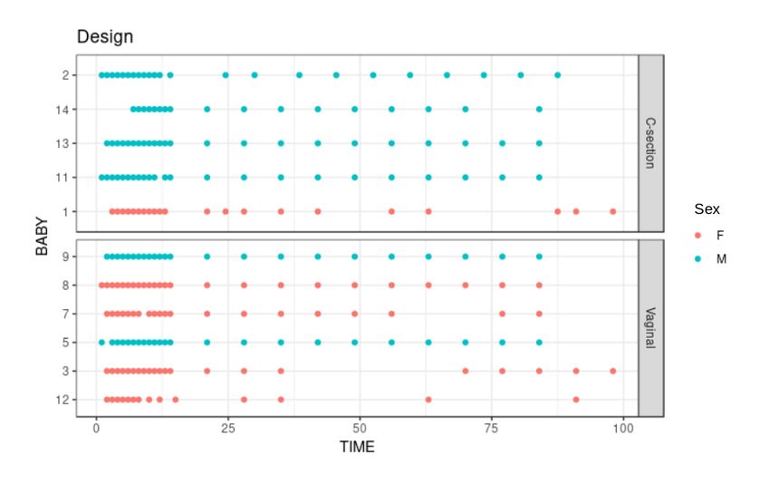
bioRxiv preprint first posted online Mar. 24, 2019; doi: http://dx.doi.org/10.1101/585802. The copyright holder for this preprint
 (which was not peer-reviewed) is the author/funder, who has granted bioRxiv a license to display the preprint in perpetuity.
                                    All rights reserved. No reuse allowed without permission.

    Figure 1: Workflow diagram for longitudinal integration of microbiota studies. We consider studies for
    the analysis of the microbiota through OTU (16S amplicon) or gene (whole genome shotgun) counts. This
    information can be complemented by additional information at the microbiota level, such as metabolic
    pathways measured with metabolomics, or information measured at a macroscopic level resulting from the
    aggregated actions of the microbiota.

    1. Low Count Removal: Only OTUs whose proportional counts exceeded 0.01% in at least one sample
       were considered for analysis. This step aims to counteract sequencing errors (Kunin et al., 2010).
    2. Total Sum Scaling (TSS) can be considered as a ‘normalisation’ process to account for uneven se-
       quencing depth across samples. TSS divides each OTU count by the total number of counts in each
       individual sample but generates compositional data expressed as proportions.
    3. Centered Log Ratio transformation addresses in a practical way the compositionality issue, by pro-
       jecting the data into a Euclidean space (Aitchison, 1982; Fernandes et al., 2014; Gloor et al., 2017).

    2.2      Time profile modelling
    2.2.1     Linear Mixed Model splines (LMMS)
    The LMMS modelling approach proposed by Straube et al. (2015) takes into account between and within
    individual variability and irregular time sampling. LMMS is based on a linear mixed model representation
    of penalised splines (Durbán et al., 2005) for different types of models. Through this flexible approach
    of serial fitting, LMMS avoids under- or over-smoothing. Briefly, four types of models are consecutively
    fitted in our framework on the TSS-CLR data:
    (1) A simple linear regression of taxa abundance on time, estimated via ordinary linear least squares - a
        straight line that assumes the response is not affected by individual variation.

                                                                       3
bioRxiv preprint first posted online Mar. 24, 2019; doi: http://dx.doi.org/10.1101/585802. The copyright holder for this preprint
(which was not peer-reviewed) is the author/funder, who has granted bioRxiv a license to display the preprint in perpetuity.
All rights reserved. No reuse allowed without permission.
(2) A penalised spline proposed by Durbán et al. (2005) to model nonlinear response patterns.
(3) A model that accounts for individual variation with the addition of a subject-specific random effect
to the mean response in model (2).
(4) An extension to model (3) that assumes individual deviations are straight lines, where individual-
specific random intercepts and slopes are fitted.
All four models are described in Appendix A. Straube et al. 2015 showed that the proportion of profiles
fitted with the different models increased in complexity with the organism considered. Different types
of splines can be considered in models (2) - (4), including a cubic spline basis (Verbyla et al., 1999), a
penalised spline and a cubic penalised spline. A cubic spline basis uses all inner time points of the measured
time interval as knots, and is appropriate when the number of time points is small (≤ 5), whereas the
penalised spline and cubic penalised spline bases use the quantiles of the measured time interval as knots,
see Ruppert (2002). In our case studies, we used penalised splines. The LMMS models are implemented
in the R package lmms (Straube et al., 2016).
2.2.2 Prediction and interpolation
The fitted splines enable us to predict or interpolate time points that might be missing within the time
interval (e.g. inconsistent time points between different types of data or covariates). Additionally, inter-
polation is useful in our multivariate analyses described below to smooth profiles, and when the number
of time points is small (≤ 5). In the following section, we therefore consider data matrices X (T × P ),
where T is the number of (interpolated) time points and P the number of taxa. The individual dimension
has thus been summarised through the spline fitting procedure, so that our original data matrix of size
(N × P × T ), where N is the number of biological samples, is now of size (T × P ).
2.3 Filtering profiles after modelling
A simple linear regression model (1) might be the result of highly noisy data. To retain only the most
meaningful profiles, the quality of these models was assessed with a Breusch-Pagan test to indicate whether
the homoscedasticity assumption of each linear model was met (Breusch and Pagan, 1979) . We also used
a threshold based on the mean squared error (MSE) of the linear models, by only including profiles for
which their MSE was below the maximum MSE of the more complex fitted models (1) - (4). The latter
filter was only applied when a large number of linear models (1) were fitted and the Breusch-Pagan test
was not considered stringent enough.
2.4 Clustering time profiles
2.4.1 PCA and sparse PCA
Multivariate dimension reduction techniques such as Principal Component Analysis (PCA, Jolliffe 2005)
and sparse PCA (Huang and Zheng, 2006) can be used to cluster taxa profiles. To do so, we consider as
data input the X (T × P ) spline fitted matrix. Let t1 , t2 , . . . , tH denote the H principal components of
length T and their associated v1 , v2 , . . . , vH factors - or loading vectors, of length P . For a given PCA
dimension h, we can extract a set of strongly correlated profiles by considering taxa with the top absolute
coefficients in vh . Those profiles are linearly combined to define each component th , and thus, explain
similar information on a given component. Different clusters are therefore obtained on each dimension h
of PCA, h = 1 . . . H. Each cluster h is then further separated into two sets of profiles which we denote as
’positive’ or ’negative’ based on their correlation (see Figure 3).
A more formal approach can be used with sparse PCA. Sparse PCA includes `1 penalisations on the
loading vectors to select variables that are key for defining each component, and are highly correlated
within a component (see Huang and Zheng 2006 for more details).
2.4.2 Choice of the number of clusters in PCA
We propose to use the average silhouette coefficient (Rousseeuw, 1987) to determine the optimal number
of clusters, or dimensions H, in PCA. For a given identified cluster and observation i, the silhouette
4bioRxiv preprint first posted online Mar. 24, 2019; doi: http://dx.doi.org/10.1101/585802. The copyright holder for this preprint
(which was not peer-reviewed) is the author/funder, who has granted bioRxiv a license to display the preprint in perpetuity.
All rights reserved. No reuse allowed without permission.
coefficient of i is defined as
b(i) − a(i)
s(i) = (5)
max(a(i), b(i))
where a(i) is the average distance between observation i and all other observations within the same cluster,
and b(i) is the average distance between observation i and all other observations in the nearest cluster.
A silhouette score is obtained for each observation and averaged across all silhouette coefficients, ranging
from -1 (poor) to 1 (good clustering).
We adapted the silhouette coefficient to choose the number of components or clusters in PCA and
sPCA (i.e. 2 × H clusters), as well as the number of profiles to select for each cluster. Each observation
in Eq. (5) now represents a fitted LMMS profile, and the distance between two profiles is calculated using
the Spearman Correlation coefficient.
Within a given cluster, we calculate the silhouette coefficient of each LMMS profile and apply the
following empirical rules for cluster assignation: a coefficient > 0.5 assigns the profile to the cluster, a
value between 0 and 0.5 indicates an uncertain assignment as the profile can be assigned to one or two
clusters, while a negative value indicates that the profile should not be assigned to this particular cluster.
To choose the appropriate number of profiles per sPCA component, we perform as follows: For each
component, we set a grid of number of profiles to be retained with sPCA and calculated the average
silhouette coefficient per cluster (there are two clusters per component). The final number of profiles to se-
lect is arbitrarily set when we observe a sudden decrease in the average silhouette coefficient (see Figure 4).
We also used the average silhouette coefficient to assess the quality of different clustering approaches,
as illustrated in the Results Section: a greater average silhouette coefficient indicates a better clustering
of the profiles.
2.5 Integration
2.5.1 Multiblock PLS methods
To integrate multiple datasets (also called blocks) measured on the same biological samples we used multi-
variate methods based on Projection to Latent Structures (PLS) methods (Wold, 1975), which we broadly
term multiblock PLS approaches. For example, we can consider Generalised Canonical Correlation Anal-
ysis (GCCA, Tenenhaus and Tenenhaus 2011; Tenenhaus et al. 2014), which, contrary to what its name
suggests, generalises PLS for the integration of more than two datasets. Recently, we have developed the
DIABLO method to discriminate different phenotypic groups in a supervised framework (Singh et al.,
2019). In the context of this study however, we present the sparse GCCA in an unsupervised framework,
where input datasets are spline-fitted matrices.
We denote Q data sets X (1) (T × P1 ), X (2) (T × P2 ), ..., X (Q) (T × PQ ) measuring the expression levels of
Pq variables of different types (taxa, ‘omics, continuous response of interest), modelled on T (interpolated)
time points, q = 1, . . . , Q. GCCA solves for each component h = 1, . . . , H:
Q
(q) (q) (j) (j) (q) (q)
X
max cq,j cov(Xh ah , Xh ah ), s.t. ||ah ||2 = 1 and ||ah ||1 ≤ λ(q) (6)
(1) (Q)
ah ,...,ah q,j=1,q6=j
(q)
where λ(q) is the `1 penalisation parameter, ah is the loading vector on component h associated with the
(q)
residual (deflated) matrix Xh of the data set X (q) , and C = {cq,j }q,j is the design matrix. C is a Q × Q
matrix that specifies whether datasets should be correlated and includes values between zero (datasets are
not connected) and one (datasets are fully connected). Thus, we can choose to take into account specific
pairwise covariances by setting the design matrix (see Rohart et al. 2017 for implementation and usage)
and model a particular association between pairs of datasets, as expected from prior biological knowledge
or experimental design. In our integrative case study, we used sparse PLS, a special case of Eq. (6) to
integrate microbiome and metabolomic data, as well as sparse multiblock PLS to also integrate variables
of interest. Both methods were used with a fully connected design.
5bioRxiv preprint first posted online Mar. 24, 2019; doi: http://dx.doi.org/10.1101/585802. The copyright holder for this preprint
(which was not peer-reviewed) is the author/funder, who has granted bioRxiv a license to display the preprint in perpetuity.
All rights reserved. No reuse allowed without permission.
The multiblock sparse PLS method was implemented in the mixOmics R package where the `1 penali-
sation parameter is replaced by the number of variables to select, using a soft-thresholding approach (see
more details in Rohart et al. 2017).
2.5.2 Parameters tuning
(q) (q) (q)
The integrative methods require choosing the number of components H, defined as th = ah Xh with
the notations from Section 2.5.1, and number of profiles to select on each PLS component and in each
dataset. We generalised the approach described in Section 2.4.2 using the silhouette coefficient based on
a grid of parameters for each dataset and each component.
2.6 Case studies
2.6.1 Infant gut microbiota development
The gastrointestinal microbiome of 14 babies during the first year of life was studied by Palmer et al.
(2007). The authors collected an average of 26 stool samples from healthy full-term infants. As infants
quickly reach an adult-like microbiota composition, we focused our analyses on the first 100 days of life.
Infants who received an antibiotic treatment during that period were removed from the analysis, as an-
tibiotics can drastically alter microbiome composition (Dudek-Wicher et al., 2018).
The dataset we analysed included 21 time points on average for 11 selected infants (Figure 2). Samples
were collected daily during days 0-14 and weekly after the second week. We separated our analyses based
on the delivery mode (C-section or vaginal), as this is known to have a strong impact on gut microbiota
colonisation patterns and diversity in early life (Rutayisire et al. (2016)).
Figure 2: Infant gut microbiota development study: stool samples were collected from six male and five
female babies over the course of 100 days. Samples were collected daily during days 0-14 and weekly
thereon until day 100. Time is indicated on the x-axis in days. As delivery method is known to be a strong
influence on gut microbiome colonisation, the data are separated according to either C-section or vaginal
birth.
2.6.2 Waste degradation study
Anaerobic digestion (AD) is a highly relevant microbial process to convert waste into valuable biogas. It in-
volves a complex microbiome that is responsible for the progressive degradation of molecules into methane
and carbon dioxide. In this study, AD’s biowaste was monitored across time (more than 150 days) in three
lab-scale bioreactors as described in (Poirier et al., 2016). The purpose of the study was to investigate the
6bioRxiv preprint first posted online Mar. 24, 2019; doi: http://dx.doi.org/10.1101/585802. The copyright holder for this preprint
(which was not peer-reviewed) is the author/funder, who has granted bioRxiv a license to display the preprint in perpetuity.
All rights reserved. No reuse allowed without permission.
relationship between biowaste degradation performance, microbial dynamics and metabolomic dynamics
across time.
We focused our analysis on days 9 to 57, that correspond to the most intense biogas production.
Degradation performance was monitored through 4 parameters: methane and carbon dioxide production
(16 time points) and accumulation of acetic and propionic acid in the bioreactors (5 time points). Microbial
dynamics were profiled with 16S RNA gene metabarcoding as described in Poirier et al. (2016) and included
4 time points and 90 OTUs. A metabolomic assay was conducted on the same biological samples on 4
time points with gas chromatography coupled to mass spectrometry GC-MS after solid phase extraction
to monitor substrates degradation (Limam et al., 2010). The XCMS R package (version 1.52.0) was used to
process the raw metabolomics data (Smith et al., 2006). GC-MS analyses focused on 20 peaks of interest
identified by the National Institute of Standards and Technology database. Data were then log-transformed
for statistical analysis.
3 Results
3.1 Clustering time profiles: Infant gut microbiota development study
3.1.1 Pre-processing and modelling
A total of 2,149 taxa were identified in the raw data (Table 1). After the pre-processing steps illustrated in
Figure 1, a smaller number of OTUs were found in faecal samples of babies born by C-section than vaginal
delivery. Similarly, a simple linear regression model showed a smaller proportion of OTUs in babies born
via C-section (73%) than vaginal delivery (81%), and this was also observed after the filtering step (Table
1).
3.1.2 Comparison of PCA and functional PCA
Functional Principal Component Analysis (fPCA) was proposed by Ramsay and Silverman (2005) and
is a popular approach to cluster longitudinal data (Jacques and Preda, 2014). fPCA extracts ‘modes of
variation’ and performs functional clustering and identification of longitudinal data sub-structures using k-
centres functional Clustering (k-CFC, Chiou and Li 2007 or model-based clustering using an Expectation-
Maximization algorithm (Chen et al., 2012). Both clustering methods are implemented in fdapace R
package (Dai et al., 2018).
Based on the silhouette coefficient, we included 4 clusters (i.e. two components) in PCA, and set the
same number of clusters in fPCA for comparative purposes. PCA clustering outperformed fPCA for each
delivery mode dataset that was analysed (see Table 2). The resulting fPCA clustering is displayed in
Figure 4 for babies born via vaginal delivery. We found that the EM approach in fPCA tended to cluster
a larger number of uncorrelated OTUs compared to the k-CFC approach (average silhouette coefficient =
0.07 for EM and 0.61 for k-CFC).
3.1.3 Clusters of profiles
We used sPCA to select key OTU profiles for each cluster. This step is essential for discarding profiles that
are distant from the average cluster profile and thus not informative. As expected, we observed an overall
increase in the silhouette average coefficient for the sPCA clustering compared to PCA, indicating a better
clustering capability (see Table 2). According to the silhouette average coefficient, vaginal delivery showed
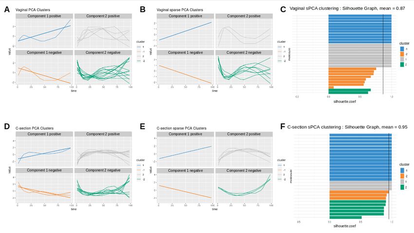
the best partitioning for PCA clustering (0.87, Table 2). Cluster 1 (denoted ‘component 1 positive’ in
Figure 3 A) showed an increase in the abundance profile of species, including some that are characteristic
of a healthy “adult-like” gut microbiome composition such as the clade Bacteroidetes (Thursby and Juge,
2017). In cluster 2 (‘component 1 negative’), profile abundance tended to decrease and corresponded to
genera found in abundance in vaginal and skin microbiota, such as Lactobacillus and Propionibacterium
(Grice and Segre, 2011; Bing et al., 2012). Clusters 3 and 4 (denoted ‘component 2 positive and neg-
ative’) highlighted taxa with negatively correlated profiles. Thus, with this preliminary PCA analysis,
we were able to rebuild a partial history behind the development of the gut microbiota. Vaginal species
that initially colonized in the gut progressively disappeared to enable species that characterize adult gut
7bioRxiv preprint first posted online Mar. 24, 2019; doi: http://dx.doi.org/10.1101/585802. The copyright holder for this preprint
(which was not peer-reviewed) is the author/funder, who has granted bioRxiv a license to display the preprint in perpetuity.
All rights reserved. No reuse allowed without permission.
Figure 3: Vaginal (first row) and C-section delivery babies (second row). (A) - (B), (D) - (E): OTU profiles
clustered with either PCA or sPCA. Each line represents the abundance of a selected OTU across time.
OTUs were clustered according to their contribution on each component for PCA, and `1 penalisation
for sPCA. The PCA clusters were further separated into profiles with a positive or negative correlation.
Profiles were scaled to improve visualisation. (C) - (F): Silhouette profile for each identified clustering.
Each bar represents the silhouette coefficient of a particular OTU and colors represent assigned clusters.
The average coefficient is represented by a vertical black line. A greater average silhouette coefficient
means a better partitioning state. (C): vaginal delivery babies with sPCA (average silhouette coefficient
= 0.87); (F): C-section delivery babies with sPCA (average silhouette coefficient = 0.95).
microbiota.
For babies born by C-section, 4 clusters were identified by PCA (Fig. 3 D). Clusters 1 and 2 (‘com-
ponent 1 positive and negative’) displayed a clear increase and decrease respectively in abundance profile.
However none of the cluster 2 species are known to characterize, or were found in, vaginal delivery, sug-
gesting that the infant gut was first colonized by the operating room microbes as already demonstrated by
Shin et al. (2015). Cluster 3 (‘component 2 positive’) revealed transitory states of increase then decrease
of abundance profiles, while cluster 4 (‘component 2 negative’) showed a decrease then an increase.
3.2 Clustering omics: waste degradation study
3.2.1 Pre-processing and modelling
A total of ninety OTUs were identified in the 12 samples of the initial dataset (Table 4). After pre-
processing, 51 OTUs were retained. Approximately 60% (resp. 50%) of the OTUs (resp. metabolites)
were fitted with linear regression models (1) and 40% (resp. 50%) were modelled by more complex splines
models (2) - (4). All performance measures were also modelled by splines. During the filtering step, 7
OTUs and 4 metabolites that were fitted with linear regression models were discarded.
3.2.2 sPCA on concatenated datasets
As a first and naive attempt to jointly analyse microbial, metabolomic and performance measures, all
three datasets were concatenated then analysed with sPCA. Only a very small number of profiles from the
8bioRxiv preprint first posted online Mar. 24, 2019; doi: http://dx.doi.org/10.1101/585802. The copyright holder for this preprint
(which was not peer-reviewed) is the author/funder, who has granted bioRxiv a license to display the preprint in perpetuity.
All rights reserved. No reuse allowed without permission.
Figure 4: fPCA Expectation-Maximization clustering (first row) and k- Center Functional Clustering
(second row). (A) - (C): Vaginal OTU profiles clustered with either EM or k-CFC. Each line represents
the abundance of a selected OTU across time. (B) - (D): Silhouette coefficient for each profile and each
clustering. Each bar represents the silhouette coefficient of a particular OTU and colors represent assigned
clusters. The average coefficient is represented by a vertical black line. The average silhouette coefficient
was 0.07 for EM clustering and 0.61 for k-CFC clustering.
different datasets were selected. This small selection is likely due to the high variability in each data type.
Selected variables included mainly OTUs and performance measures. These were assigned to four clusters
and included respectively 1, 3, 2 and 3 OTUs with 0, 1, 2 and 0 metabolites and 2, 0, 1 and 0 performance
measures. The average silhouette coefficient was 0.744, a potentially sub-optimal clustering compared to
our analyses presented in the next Section. This preliminary investigation highlighted the limitation of
sPCA to identify a sufficient number of correlated profiles from disparate sources.
3.2.3 Microbiome - metabolomic integration with sPLS
The results from the sPLS analysis are shown in Figure 5. Four clusters of variables were selected. The first
cluster (denoted ‘component 1 negative’) included 10 OTUs and 4 metabolite variables, and showed in-
creasing abundance until a plateau was reached at approximately 40 days. The OTUs were microorganisms
often recovered during anaerobic digestion of biowaste, such as methanogenic archaea of Methanosarcina
genus or bacteria of Clostridiales, Acholeplasmatales, and Anaerolineales orders (Poirier et al., 2016).
Their abundance increased while biowaste was degraded, until there was no more biowaste available in
the bioreactor. Their abundance was correlated to the intensity of various metabolites produced dur-
ing the AD process, such as benzoic acid that is formed during the degradation of phenolic compounds
(Hoyos-Hernandez et al., 2014), or phytanic acid, known to be produced during the fermentation of plant
materials in the ruminant gut (Watkins et al., 2010), as well as indole-2-carboxylic acid. Cluster 2 (com-
ponent 1 positive) included 10 OTUs and 4 metabolites. These profiles were negatively correlated to
Cluster 1, and their abundance decreased with time. OTUs mainly belonged to the Bacteroidales order.
They were present in the initial inoculum but did not survive in this experiment, as the operating con-
ditions or the substrate were not optimal for their growth, as observed in other studies (Madigou et al.,
2019). Metabolites identified in Cluster 2 were present in the biowaste and were degraded during the
9bioRxiv preprint first posted online Mar. 24, 2019; doi: http://dx.doi.org/10.1101/585802. The copyright holder for this preprint
(which was not peer-reviewed) is the author/funder, who has granted bioRxiv a license to display the preprint in perpetuity.
All rights reserved. No reuse allowed without permission.
experiment. They included fatty acids (decanoic and tetradecanoic acids) that can be found in oil, or
3-(3-Hydroxyphenyl)propionic acid, arising from digestion of aromatic amino-acids or breakdown product
of lignin or other plant-derived phenylpropanoids. As their profile was negatively correlated to those from
cluster 1, it is likely that these metabolites were consumed by OTUs assigned to cluster 1 (Torres et al.,
2003). Cluster 3 (component 2 negative) included 1 OTU and 5 metabolites. Profiles decreased slowly
with time. One OTU of Clostridiales order appears to have been out-competed by other OTUs or phase
active only during the first days of the degradation. Among the metabolites of this cluster, Hydrocinnamic
and 3,4-Dihydroxyhydrocinnamic acids are commonly found in plant biomass and its residues (Boerjan
et al., 2003). Their molecular structure may have contributed to their slower degradation compared to
other molecules. Finally, Cluster 4 (component 2 positive) included 11 OTUs and 3 metabolites with slow
abundance increase. OTUs of this group were very varied with 8 orders represented. They may have slower
growth rates than OTUs of cluster 1 or were involved in the last steps of the degradation. Metabolites
included N-Acetylanthranilic acid and Dehydroabietic acid that were likely produced by microorganisms
and accumulated during the anaerobic digestion process. The average silhouette coefficient was 0.954 and
confirmed that sPLS led to better clustering of the different types of profiles than sPCA in Section 3.2.2.
Figure 5: Biowaste study: sPLS analysis identified correlated profiles of OTUs and metabolites. Each
line represents the abundance of selected OTUs and metabolites across time. OTUs and metabolites were
clustered according to their contribution on each component for sPLS. The clusters were further separated
into profiles with a positive or negative correlation.
3.2.4 Microbiome, metabolomic and performance data integration with block sPLS
Figure 6 illustrates the results from the integration of the three datasets, where the performance data are
considered as the response of interest. Similar to the sPLS analysis, block sPLS assigned profiles to four
clusters, with an average silhouette coefficient of 0.909. Two performance variables (methane and carbon
dioxyde production) were assigned to cluster 1. This result is biologically relevant, as biogas is the final
output of the AD reaction and is known to be associated with microbial activity and growth. Moreover,
it is produced by archaea, such as Methanosarcina, also selected in this cluster. In Cluster 2 (component
2 negative), we identified acetate produced by bacteria in the early days of the incubation and consumed
by archaea (Cluster 1) to produce biogas. Propionate was assigned to the third cluster, as its degradation
10bioRxiv preprint first posted online Mar. 24, 2019; doi: http://dx.doi.org/10.1101/585802. The copyright holder for this preprint
(which was not peer-reviewed) is the author/funder, who has granted bioRxiv a license to display the preprint in perpetuity.
All rights reserved. No reuse allowed without permission.
only starts when all acetate is degraded (Chapleur et al., 2014). Cluster 4 was composed of only OTUs
and metabolites and was similar to the one obtained with sPLS.
Figure 6: Biowaste degradation study: integration of OTUs, metabolites and performance measures with
block sPLS. Each line represents the abundance of selected OTUs, metabolites and performance measures
across time. OTUs, metabolites and performance measures were clustered according to their contribution
on each component for block sPLS. The clusters were further separated into profiles with a positive or
negative correlation.
4 Discussion
Advances in technology and reduced sequencing costs have resulted in the emergence of new and more
complex experimental designs that combine multiple omic datasets and several sampling times from the
same biological material. Thus, the challenge is to integrate longitudinal, multi-omic data to capture the
complex interactions between these omic layers and obtain a holistic view of biological systems. In order
to integrate longitudinal data from microbial communities with other omics, meta-omics or other clinical
variables, we proposed a data-driven analytical framework to identify highly correlated temporal profiles
between these multiple and heterogeneous datasets.
In the proposed framework, the microbial counts of the microbiota’s constituent species are normalised
for uneven sequencing library sizes and compositional data. Modelling with linear mixed model splines
enables us to reduce the dimension of the data across the different biological replicates and take into
account the individual variability due to either technical or biological sources. This approach also en-
ables us to compare data analysed at different time points (e.g bioreactor study). Lastly, we clustered
the data using multivariate dimension reduction techniques on the spline models that further allowed in-
tegration between different data types, and the identification of the main patterns of longitudinal variation.
A similar approach to ours was proposed by Ribicic et al. (2018) who used linear regression models
coupled with multivariate dimension reduction methods on 16S and chemical longitudinal data to study
the effects of oil temperature and composition on the biodegradation of chemically dispersed oil. We have
11bioRxiv preprint first posted online Mar. 24, 2019; doi: http://dx.doi.org/10.1101/585802. The copyright holder for this preprint
(which was not peer-reviewed) is the author/funder, who has granted bioRxiv a license to display the preprint in perpetuity.
All rights reserved. No reuse allowed without permission.
taken their approach one step further, with the appropriate handling of compositional data, a fully devel-
oped modelling framework, and the identification of key profiles assigned to different clusters using sparse
multivariate integrative methods.
Integrating different types of microbiome longitudinal data (abundance, activity, metabolic pathways,
macroscopic output...) can be naively performed by concatenating all datasets. However, we showed that
this approach was unsuccessful at selecting a sufficiently large number of profiles of different types, and
thus does not shed light on the holistic view of the ecosystem dynamics (bioreactor study). Our integrative
multivariate methods sPLS and block sPLS are better suited for the integration task, as they do not merge
but rather statistically correlate components built on each dataset, and avoid unbalance in the signature
when one dataset might be either more informative, less noisy, or larger than the other datasets.
When compared with fPCA, that uses either k-CFC or EM clustering algorithms, we showed that our
approach led to better clustering performance. In addition, the sparse multivariate approaches sPCA and
block sPLS enable the identification of key profiles to improve biological interpretation. Note however that
fPCA might be better suited than our approach for a large number of time points, as we discuss next.
We have identified several limitations in our proposed framework. Firstly, a high individual variability
between biological replicates limits the LMMS modelling step, resulting in simple linear regression models
to fit the data. Whilst a straight line model may accurately describe temporal dynamics, it could also
be due to a poor quality of fit. We have implemented the Breusch-Pagan test to address this issue. Al-
ternatively, in the case of a very high inter-individual variability that prevents appropriate smoothing,
one could consider N of One analyses as proposed by Gerber et al. (2012); Äijö et al. (2017) with time
dynamical probabilistic models. Secondly, a large number of time points can result in the modelling of
noisy profiles and clusters, often due to high individual variability. Highly variable and vastly different
profiles can also be difficult to cluster appropriately. Therefore, this framework is recommended when the
number of time points remains small (5-10) and when regular and similar trends are expected from the
data. Thirdly, our framework does not include time delay analysis, even though dynamic delays between
different types of molecules (e.g. DNA, RNA, metabolites...) can be expected. For example, 16S data
describes the abundance of the microorganisms while metabolites are the consequences of their activity,
and performances are the macroscopic resulting output. Potential delays between these molecules can be
detected using other techniques, such as the Fast Fourier Transform approach from Straube et al. (2017)
and will be further investigated in our future work.
To summarise, we have proposed one of the first computational framework to integrate longitudinal
microbiome data with other omics data or other variables generated on the same biological samples or
material. The identification of highly-correlated key omics features can help generate novel hypotheses to
better understand the dynamics of biological and biosystem interactions. Thus, our data-driven approach
will open new avenues for the exploration and analyses of multi-omics studies.
Conflict of Interest Statement
The authors declare that the research was conducted in the absence of any commercial or financial rela-
tionships that could be construed as a potential conflict of interest.
Author Contributions
All authors contributed to the design of the study; AB and OC performed the statistical analyses; AB,
OC and KALC wrote the manuscript. All authors contributed to manuscript revision, read and approved
the submitted version.
Funding
KALC was supported in part by the National Health and Medical Research Council (NHMRC) Career
Development fellowship (GNT1159458). KALC and OC scientific travels were supported in part by the
France-Australia Science Innovation Collaboration (FASIC) Program Early Career Fellowships from the
12bioRxiv preprint first posted online Mar. 24, 2019; doi: http://dx.doi.org/10.1101/585802. The copyright holder for this preprint
(which was not peer-reviewed) is the author/funder, who has granted bioRxiv a license to display the preprint in perpetuity.
All rights reserved. No reuse allowed without permission.
Australian Academy of Science. AD was supported by Research and Innovation chair L’Oreal in Digital
Biology.
Acknowledgments
We thank Angéline Guenne for analytical support with GC-MS analysis, Kodjovi Dodji Mlaga for the
biological interpretations of the infant study, and Zoe Welham for proof-reading the manuscript.
Supplemental Data
Data Availability Statement
Infant gut microbiota phylochip raw data can be found in Palmer et al. (2007). The microbiome and
performance datasets for the bioreactor study can be found in Poirier and Chapleur (2018), metabolomic
data is available on request. In-house scripts and code to conduct both case study analysis, are available
in a Github public repository : https://github.com/abodein/timeOmics
Table 1: Number of OTUs identified, and linear model types fitted according to delivery mode.
C-section Vaginal
Identified OTUs 2,149 2,149
# OTUs after pre-processing 107 117
Linear model types (1) 78 95
(2) 29 22
Linear model types after filtering 1 42 68
2 29 22
Table 2: Average silhouette coefficient according to clustering method
PCA sPCA fPCA (k-CFC) fPCA(EM)
Vaginal 0.84 0.95 0.61 0.07
C-section 0.87 0.86 0.69 0.35
Table 3: Number of OTUs per cluster identified with PCA clustering and OTUs selected in brackets with
sparce PCA.
C-section Vaginal
Cluster 1 (comp 1 positive) 11 (3) 32 (9)
Cluster 2 (comp 1 negative) 35 (15) 38 (11)
Cluster 3 (comp 2 positive) 15 (6) 6 (2)
Cluster 4 (comp 2 negative) 10 (3) 14 (8)
References
Äijö, T., Müller, C. L., and Bonneau, R. (2017). Temporal probabilistic modeling of bacterial compositions derived from 16s rrna
sequencing. Bioinformatics, 34(3), 372–380.
Aitchison, J. (1982). The statistical analysis of compositional data. Journal of the Royal Statistical Society. Series B (Method-
ological), pages 139–177.
Baksi, K. D., Kuntal, B. K., and Mande, S. S. (2018). ‘time’: A web application for obtaining insights into microbial ecology using
longitudinal microbiome data. Frontiers in Microbiology, 9, 36.
Bing, M., Forney, L., and Ravel, J. (2012). The vaginal microbiome: rethinking health and diseases. Annu Rev Microbiol, 66,
371–89.
Boerjan, W., Ralph, J., and Baucher, M. (2003). Lignin biosynthesis. Annual review of plant biology, 54(1), 519–546.
13bioRxiv preprint first posted online Mar. 24, 2019; doi: http://dx.doi.org/10.1101/585802. The copyright holder for this preprint
(which was not peer-reviewed) is the author/funder, who has granted bioRxiv a license to display the preprint in perpetuity.
All rights reserved. No reuse allowed without permission.
Table 4: OTUs, metabolites and performance modelling and filtering in the bioreactor study. Only OTUs
data were preprocessed.
Type of features OTUs Metabolites Performance
Number of features 90 20 4
# features after pre-processing 51 NA NA
Linear model types (1) 30 10 0
(2) 19 0 2
(3) 2 4 0
(4) 0 6 2
Linear model types after filtering (1) 24 6 0
(2) 19 0 2
(3) 2 4 0
(4) 0 6 2
Breusch, T. S. and Pagan, A. R. (1979). A simple test for heteroscedasticity and random coefficient variation. Econometrica:
Journal of the Econometric Society, pages 1287–1294.
Bucci, V., Tzen, B., Li, N., Simmons, M., Tanoue, T., Bogart, E., Deng, L., Yeliseyev, V., Delaney, M. L., Liu, Q., et al. (2016).
Mdsine: Microbial dynamical systems inference engine for microbiome time-series analyses. Genome biology, 17(1), 121.
Caporaso, J. G., Kuczynski, J., Stombaugh, J., Bittinger, K., Bushman, F. D., Costello, E. K., Fierer, N., Pena, A. G., Goodrich,
J. K., Gordon, J. I., et al. (2010). Qiime allows analysis of high-throughput community sequencing data. Nature methods, 7(5),
335.
Chapleur, O., Bize, A., Serain, T., Mazéas, L., and Bouchez, T. (2014). Co-inoculating ruminal content neither provides active
hydrolytic microbes nor improves methanization of 13c-cellulose in batch digesters. FEMS microbiology ecology, 87(3), 616–629.
Chen, W., Maitra, R., and Melnykov, V. (2012). EMCluster: EM Algorithm for Model-Based Clustering of Finite Mixture Gaussian
Distribution.
Chiou, J.-M. and Li, P.-L. (2007). Functional clustering and identifying substructures of longitudinal data. Journal of the Royal
Statistical Society: Series B (Statistical Methodology), 69(4), 679–699.
Clemmensen, L., Hastie, T., Witten, D., and Ersbøll, B. (2011). Sparse discriminant analysis. Technometrics, 53(4), 406–413.
Dai, X., Hadjipantelis, P. Z., Han, K., and Ji, H. (2018). fdapace: Functional Data Analysis and Empirical Dynamics. R package
version 0.4.0.
Dudek-Wicher, R. K., Junka, A., and Bartoszewicz, M. (2018). The influence of antibiotics and dietary components on gut microbiota.
Przeglad gastroenterologiczny, 13(2), 85.
Durbán, M., Harezlak, J., Wand, M., and Carroll, R. (2005). Simple fitting of subject-specific curves for longitudinal data. Statistics
in medicine, 24(8), 1153–1167.
Escudié, F., Auer, L., Bernard, M., Mariadassou, M., Cauquil, L., Vidal, K., Maman, S., Hernandez-Raquet, G., Combes, S., and
Pascal, G. (2017). Frogs: find, rapidly, otus with galaxy solution. Bioinformatics, 34(8), 1287–1294.
Faust, K., Lahti, L., Gonze, D., De Vos, W. M., and Raes, J. (2015). Metagenomics meets time series analysis: unraveling microbial
community dynamics. Current opinion in microbiology, 25, 56–66.
Fernandes, A. D., Reid, J. N., Macklaim, J. M., McMurrough, T. A., Edgell, D. R., and Gloor, G. B. (2014). Unifying the analysis
of high-throughput sequencing datasets: characterizing rna-seq, 16s rrna gene sequencing and selective growth experiments by
compositional data analysis. Microbiome, 2(1), 15.
Fukuyama, J., Rumker, L., Sankaran, K., Jeganathan, P., Dethlefsen, L., Relman, D. A., and Holmes, S. P. (2017). Multidomain
analyses of a longitudinal human microbiome intestinal cleanout perturbation experiment. PLoS computational biology, 13(8),
e1005706.
Gavin, P., Mullaney, J., Loo, D., Lê Cao, K.-A., Gottlieb, P., Hill, M., Zipris, D., and Hamilton-Williams, E. (2018). Intestinal
metaproteomics reveals host-microbiota interactions in subjects at risk for type 1 diabetes. DIABETES CARE , 41, 2178–2186.
Gerber, G. K., Onderdonk, A. B., and Bry, L. (2012). Inferring dynamic signatures of microbes in complex host ecosystems. PLoS
computational biology, 8(8), e1002624.
Gloor, G. B., Macklaim, J. M., Pawlowsky-Glahn, V., and Egozcue, J. J. (2017). Microbiome datasets are compositional: and this
is not optional. Frontiers in microbiology, 8, 2224.
Grice, E. A. and Segre, J. A. (2011). The skin microbiome. Nature Reviews Microbiology, 9(4), 244.
Guidi, L., Chaffron, S., Bittner, L., Eveillard, D., Larhlimi, A., Roux, S., Darzi, Y., Audic, S., Berline, L., Brum, J. R., et al. (2016).
Plankton networks driving carbon export in the oligotrophic ocean. Nature, 532(7600), 465.
14bioRxiv preprint first posted online Mar. 24, 2019; doi: http://dx.doi.org/10.1101/585802. The copyright holder for this preprint
(which was not peer-reviewed) is the author/funder, who has granted bioRxiv a license to display the preprint in perpetuity.
All rights reserved. No reuse allowed without permission.
Hoyos-Hernandez, C., Hoffmann, M., Guenne, A., and Mazeas, L. (2014). Elucidation of the thermophilic phenol biodegradation
pathway via benzoate during the anaerobic digestion of municipal solid waste. Chemosphere, 97, 115–119.
Huang, D.-S. and Zheng, C.-H. (2006). Independent component analysis-based penalized discriminant method for tumor classification
using gene expression data. Bioinformatics, 22(15), 1855–1862.
Jacques, J. and Preda, C. (2014). Functional data clustering: a survey. Advances in Data Analysis and Classification, 8(3),
231–255.
Jolliffe, I. (2005). Principal component analysis. Wiley Online Library.
Knight, R., Jansson, J., Field, D., Fierer, N., Desai, N., Fuhrman, J. A., Hugenholtz, P., Van Der Lelie, D., Meyer, F., Stevens, R.,
et al. (2012). Unlocking the potential of metagenomics through replicated experimental design. Nature biotechnology, 30(6), 513.
Kunin, V., Engelbrektson, A., Ochman, H., and Hugenholtz, P. (2010). Wrinkles in the rare biosphere: pyrosequencing errors can
lead to artificial inflation of diversity estimates. Environmental microbiology, 12(1), 118–123.
Lê Cao, K., Rossouw, D., Robert-Granié, C., Besse, P., et al. (2008). A sparse PLS for variable selection when integrating omics
data. Statistical applications in genetics and molecular biology, 7, Article–35.
Limam, I., Guenne, A., Driss, M. R., and Mazéas, L. (2010). Simultaneous determination of phenol, methylphenols, chlorophenols
and bisphenol-a by headspace solid-phase microextraction-gas chromatography-mass spectrometry in water samples and industrial
effluents. International Journal of Environmental and Analytical Chemistry, 90(3-6), 230–244.
Luo, D., Ziebell, S., and An, L. (2017). An informative approach on differential abundance analysis for time-course metagenomic
sequencing data. Bioinformatics, 33(9), 1286–1292.
Lê Cao, K.-A., Costello, M.-E., Lakis, V. A., Bartolo, F., Chua, X.-Y., Brazeilles, R., and Rondeau, P. (2016a). Mixmc: a multivariate
statistical framework to gain insight into microbial communities. PloS one, 11(8), e0160169.
Lê Cao, K.-A., Costello, M.-E., Chua, X.-Y., Brazeilles, R., and Rondeau, P. (2016b). Mixmc: Multivariate insights into microbial
communities. PLoS ONE , 11(8), e0160169.
Madigou, C., Lê Cao, K.-A., Bureau, C., Mazéas, L., Déjean, S., and Chapleur, O. (2019). Ecological consequences of abrupt
temperature changes in anaerobic digesters. Chemical Engineering Journal, 361, 266–277.
Metwally, A. A., Yang, J., Ascoli, C., Dai, Y., Finn, P. W., and Perkins, D. L. (2018). Metalonda: a flexible r package for identifying
time intervals of differentially abundant features in metagenomic longitudinal studies. Microbiome, 6(1), 32.
Morris, A., Paulson, J. N., Talukder, H., Tipton, L., Kling, H., Cui, L., Fitch, A., Pop, M., Norris, K. A., and Ghedin, E. (2016).
Longitudinal analysis of the lung microbiota of cynomolgous macaques during long-term shiv infection. Microbiome, 4(1), 38.
Palmer, C., Bik, E. M., DiGiulio, D. B., Relman, D. A., and Brown, P. O. (2007). Development of the human infant intestinal
microbiota. PLoS biology, 5(7), e177.
Paulson, J. N., Talukder, H., and Bravo, H. C. (2017). Longitudinal differential abundance analysis of microbial marker-gene surveys
using smoothing splines. BioRxiv , page 099457.
Poirier, S. and Chapleur, O. (2018). Inhibition of anaerobic digestion by phenol and ammonia: Effect on degradation performances
and microbial dynamics. Data in brief , 19, 2235–2239.
Poirier, S., Desmond-Le Quéméner, E., Madigou, C., Bouchez, T., and Chapleur, O. (2016). Anaerobic digestion of biowaste under
extreme ammonia concentration: identification of key microbial phylotypes. Bioresource technology, 207, 92–101.
Ramsay, J. and Silverman, B. (2005). Functional data analysis. 2nd springer. New York .
Ribicic, D., McFarlin, K. M., Netzer, R., Brakstad, O. G., Winkler, A., Throne-Holst, M., and Størseth, T. R. (2018). Oil type
and temperature dependent biodegradation dynamics-combining chemical and microbial community data through multivariate
analysis. BMC microbiology, 18(1), 83.
Ridenhour, B. J., Brooker, S. L., Williams, J. E., Van Leuven, J. T., Miller, A. W., Dearing, M. D., and Remien, C. H. (2017).
Modeling time-series data from microbial communities. The ISME journal, 11(11), 2526.
Rohart, F., Gautier, B., Singh, A., and Lê Cao, K.-A. (2017). mixomics: an r package for ‘omics feature selection and multiple data
integration. PLoS Computational Biology, 13(11).
Rousseeuw, P. J. (1987). Silhouettes: a graphical aid to the interpretation and validation of cluster analysis. Journal of computational
and applied mathematics, 20, 53–65.
Ruppert, D. (2002). Selecting the number of knots for penalized splines. Journal of computational and graphical statistics, 11(4),
735–757.
Rutayisire, E., Huang, K., Liu, Y., and Tao, F. (2016). The mode of delivery affects the diversity and colonization pattern of the
gut microbiota during the first year of infants’ life: a systematic review. BMC gastroenterology, 16(1), 86.
Shields-Cutler, R. R., Al-Ghalith, G. A., Yassour, M., and Knights, D. (2018). Splinectomer enables group comparisons in longitudinal
microbiome studies. Frontiers in microbiology, 9, 785.
15bioRxiv preprint first posted online Mar. 24, 2019; doi: http://dx.doi.org/10.1101/585802. The copyright holder for this preprint
(which was not peer-reviewed) is the author/funder, who has granted bioRxiv a license to display the preprint in perpetuity.
All rights reserved. No reuse allowed without permission.
Shin, H., Pei, Z., Martinez, K. A., Rivera-Vinas, J. I., Mendez, K., Cavallin, H., and Dominguez-Bello, M. G. (2015). The first
microbial environment of infants born by c-section: the operating room microbes. Microbiome, 3(1), 59.
Singh, A., Gautier, B., Shannon, C., Rohart, F., Vacher, M., S, T., and Lê Cao, K.-A. (2019). Diablo: an integrative approach for
identifying key molecular drivers from multi-omic assays. Bioinformatics, bty1054.
Smith, C. A., Want, E. J., O’Maille, G., Abagyan, R., and Siuzdak, G. (2006). Xcms: processing mass spectrometry data for
metabolite profiling using nonlinear peak alignment, matching, and identification. Analytical chemistry, 78(3), 779–787.
Straube, J., Gorse, AD, P., Huang, B., and Lê Cao, K.-A. (2015). A linear mixed model spline framework for analysing time course
omics data. PLoS ONE .
Straube, J., Lê Cao, K.-A., and Huang, E. (2016). lmms: Linear Mixed Effect Model Splines for Modelling and Analysis of Time
Course Data. R package version 1.3.3.
Straube, J., Huang, B. E., and Lê Cao, K.-A. (2017). Dynomics to identify delays and co-expression patterns across time course
experiments. Scientific reports, 7, 40131.
Tenenhaus, A. and Tenenhaus, M. (2011). Regularized generalized canonical correlation analysis. Psychometrika, 76(2), 257–284.
Tenenhaus, A., Philippe, C., Guillemot, V., Le Cao, K.-A., Grill, J., and Frouin, V. (2014). Variable selection for generalized
canonical correlation analysis. Biostatistics, 15(3), 569–83.
Thursby, E. and Juge, N. (2017). Introduction to the human gut microbiota. Biochemical Journal, 474(11), 1823–1836.
Tibshirani, R. (1996). Regression shrinkage and selection via the lasso. Journal of the Royal Statistical Society. Series B (Method-
ological), pages 267–288.
Torres, B., Porras, G., Garcı́a, J. L., and Dı́az, E. (2003). Regulation of the mhp cluster responsible for 3-(3-hydroxyphenyl) propionic
acid degradation in escherichia coli. Journal of Biological Chemistry.
Verbyla, A. P., Cullis, B. R., Kenward, M. G., and Welham, S. J. (1999). The analysis of designed experiments and longitudinal
data by using smoothing splines. Journal of the Royal Statistical Society: Series C (Applied Statistics), 48(3), 269–311.
Watkins, P. A., Moser, A. B., Toomer, C. B., Steinberg, S. J., Moser, H. W., Karaman, M. W., Ramaswamy, K., Siegmund, K. D.,
Lee, D. R., Ely, J. J., et al. (2010). Identification of differences in human and great ape phytanic acid metabolism that could
influence gene expression profiles and physiological functions. BMC physiology, 10(1), 19.
Witten, D. M., Tibshirani, R., and Hastie, T. (2009). A penalized matrix decomposition, with applications to sparse principal
components and canonical correlation analysis. Biostatistics, 10(3), 515–534.
Wold, H. (1975). Path models with latent variables: The NIPALS approach. Acad. Press.
16You can also read