Improving the mean and uncertainty of ultraviolet multi-filter rotating shadowband radiometer in situ calibration factors: utilizing Gaussian ...
←
→
Page content transcription
If your browser does not render page correctly, please read the page content below
Atmos. Meas. Tech., 12, 935–953, 2019
https://doi.org/10.5194/amt-12-935-2019
© Author(s) 2019. This work is distributed under
the Creative Commons Attribution 4.0 License.

Improving the mean and uncertainty of ultraviolet multi-filter
rotating shadowband radiometer in situ calibration factors: utilizing
Gaussian process regression with a new method to estimate dynamic
input uncertainty
Maosi Chen1 , Zhibin Sun1 , John M. Davis1 , Yan-An Liu2,3,4 , Chelsea A. Corr1 , and Wei Gao1,5
1 United States Department of Agriculture UV-B Monitoring and Research Program, Natural Resource Ecology Laboratory,
Colorado State University, Fort Collins, CO 80523, USA
2 Key Laboratory of Geographic Information Science (Ministry of Education), East China Normal University,

Shanghai 200241, China
3 School of Geographic Sciences, East China Normal University, Shanghai 200241, China
4 ECNU-CSU Joint Research Institute for New Energy and the Environment, Shanghai 200062, China
5 Department of Ecosystem Science and Sustainability, Colorado State University, Fort Collins, CO 80523, USA

Correspondence: Maosi Chen (maosi.chen@colostate.edu), Zhibin Sun (zhibin.sun@colostate.edu),
and Yan-An Liu (yaliu@geo.ecnu.edu.cn)

Received: 31 August 2018 – Discussion started: 15 November 2018
Revised: 27 January 2019 – Accepted: 28 January 2019 – Published: 12 February 2019

Abstract. To recover the actual responsivity for the Ultra-         consistently better than those calculated using V0 from stan-
violet Multi-Filter Rotating Shadowband Radiometer (UV-             dard techniques (e.g., moving average). For example, the av-
MFRSR), the complex (e.g., unstable, noisy, and with gaps)          erage AOD biases of the GP method (0.0036 and 0.0032)
time series of its in situ calibration factors (V0 ) need to be     are much lower than those of the moving average method
smoothed. Many smoothing techniques require accurate in-            (0.0119 and 0.0119) at IL02 and OK02, respectively. The
put uncertainty of the time series. A new method is pro-            GP method’s absolute differences between UV-MFRSR and
posed to estimate the dynamic input uncertainty by exam-            AERONET AOD values are approximately 4.5 %, 21.6 %,
ining overall variation and subgroup means within a mov-            and 16.0 % lower than those of the moving average method
ing time window. Using this calculated dynamic input uncer-         at HI02, IL02, and OK02, respectively. The improved accu-
tainty within Gaussian process (GP) regression provides the         racy of in situ UVMRP V0 values suggests the GP solution
mean and uncertainty functions of the time series. This pro-        is a robust technique for accurate analysis of complex time
posed GP solution was first applied to a synthetic signal and       series and may be applicable to other fields.
showed significantly smaller RMSEs than a Gaussian pro-
cess regression performed with constant values of input un-
certainty and the mean function. GP was then applied to three
UV-MFRSR V0 time series at three ground sites. The method           1   Introduction
appropriately accounted for variation in slopes, noises, and
gaps at all sites. The validation results at the three test sites   While many instruments generate relatively stable data time
(i.e., HI02 at Mauna Loa, Hawaii; IL02 at Bondville, Illi-          series over short time windows, dynamic uncertainty levels,
nois; and OK02 at Billings, Oklahoma) demonstrated that             variable sampling densities, and/or different lengths of gaps
the agreement among aerosol optical depths (AODs) at the            with missing data can complicate the analysis of long-term
368 nm channel calculated using V0 determined by the GP             datasets. For example, the 5-year time series of a solar vari-
mean function and the equivalent AERONET AODs were                  ability indicator (Mg II core to wing index) shows consis-

Published by Copernicus Publications on behalf of the European Geosciences Union.
936                                         M. Chen et al.: Using GP regression to improve UV-MFRSR calibration factors

tency on the order of days but increasing noise level and           the daily calibration time series (Alexandrov et al., 2008)
gaps are observed at the month scale (Cebula et al., 1992).         to reduce the issue. Currently, UVMRP implements an out-
The time series of the geopotential scale factor, a function        lier detection and moving smoothing technique to overcome
of the geoidal potential, is also relatively stable on shorter      these issues. However, the process involves manual interac-
timescales but demonstrates a slowly increasing long-term           tion, performs unreliably during sparse and gapped periods,
pattern (Burša et al., 1997). Additionally, the time series of      and lacks the uncertainty estimation.
a ratio (F factor) for calibrating a satellite radiometer suite        Analyses of complex long-term time series, such as those
(i.e., VIIRS) shows band-specific gap distributions and vari-       of (UV-)MFRSR V0 values, must consider (i) the underly-
able trends (Cardema et al., 2012). As a result, these time         ing continuous trend (i.e., the mean function) and the cor-
series may not be described as a simple deterministic func-         responding trend uncertainty and (ii) the (dynamic) input
tion of time due to possible noise and gaps.                        uncertainty. For problem (i), there is a variety of available
   Long-term measurements of irradiance by Multi-Filter             approaches, such as local polynomial regression, smooth-
Rotating Shadowband Radiometers (MFRSRs) are also sub-              ing splines, and Gaussian process (GP) regression (Proietti,
ject to errors imposed by the factors mentioned above. The          2011). Local polynomial regression (LPR) constructs a poly-
MFRSR measures direct normal, diffuse horizontal, and to-           nomial within each local time window and fits its coefficients
tal horizontal irradiances at seven visible channels with a         by locally weighted least squares. LPR’s computational com-
roughly 10 nm full half maximum width (FHMW) (Har-                  plexity is low, and it can eliminate some of the randomness
rison and Michalsky, 1994). The Ultraviolet (UV) version            in the data (Hyndman, 2011). However, LPR may have dif-
of MFRSR measures the same three irradiance components              ficulty on the cases with varying sampling densities or gaps.
at seven UV channels (i.e., 300, 305, 311, 317, 325, 332,           In addition, LPR does not allow estimation of the trend near
and 368 nm) with a 2 nm FHMW (Gao et al., 2010). Cur-               the ends of the time series and cannot be used for forecasting
rently, the US Department of Energy (DOE) Atmospheric               (Hyndman, 2011). A spline is a piecewise polynomial func-
Radiation Measurement (ARM) Climate Research Facility               tion with continuous derivatives (Proietti, 2011), and smooth-
(Mather and Voyles, 2013), the NOAA Surface Radiation               ing splines estimate the underlying spline by minimizing the
(SURFRAD) (Augustine et al., 2005), and the US Depart-              distance between the spline and the observations while pe-
ment of Agriculture (USDA) UV-B Monitoring and Research             nalizing the roughness of the spline (Wahba, 2011). For ex-
Program (UVMRP) (Gao et al., 2010) maintain their own               ample, a cubic spline fit was used to fill the large gaps in
MFRSR and/or UV-MFRSR at multiple sites across the US.              the Mg II index time series (Viereck et al., 2004). Both LPR
To capture immediate instrument responsivity variation, the         and smoothing splines are unable to utilize the information
UVMRP performs in situ calibrations using the Langley               about the input uncertainties or to estimate the uncertainty
method (Slusser et al., 2000; Harrison and Michalsky, 1994)         associated with the trend. Unlike the two methods above,
or derived approaches (e.g., Chen et al., 2013, 2015, 2016)         GP does not restrict the class of the underlying functions be-
on (UV-)MFRSR direct beam measurements on days with                 cause it is not a parametric model (Rasmussen and Williams,
extended clear-sky periods (Gao et al., 2010).                      2006). Instead, it gives a priori probability to every possible
   Many factors contribute to the error or uncertainty of the       function based on the desired function characteristics such
Langley method, including variations in aerosol and/or other        as smoothness (Rasmussen and Williams, 2006). GP regres-
atmospheric constituents over the course of the calibration         sion assumes both the observations and the underlying func-
period (Augustine et al., 2003; Chen et al., 2015; Zhang et         tion are from one joint (prior) Gaussian distribution and de-
al., 2016), the presence of thin cirrus (Shaw, 1976), and in-       rives the underlying function distribution by conditioning the
strument errors (e.g., instrument tilt and misalignment, incor-     joint (prior) distribution on the observations (Rasmussen and
rect nighttime offset and angular corrections) (Alexandrov          Williams, 2006). The method takes the observational error
et al., 2007). Thus, the sequence of original UVMRP (UV-            into consideration and naturally gives the uncertainty of the
)MFRSR in situ calibration factors exhibits certain levels of       underlying function, making itself an appropriate tool for
noise. Among these uncertainties, variable AOD is consid-           problem (i). GP regression has been widely used in many
ered the major contributor to the variability in the Langley        fields (e.g., forecasting of mortality rates, Wu and Wang,
calibration factors obtained in typical atmospheric conditions      2018; prediction of spatial–temporal violent events, Kupilik
over the continental United States (Alexandrov et al., 2008),       and Witmer, 2018; and modeling-received signal strength for
even with careful cloud screening (e.g., Chen et al., 2014;         wireless local area network location fingerprinting, Richter
Alexandrov et al., 2004). In addition, extended cloudy peri-        and Toledano-Ayala, 2015).
ods and low solar zenith angles during winter months further           For problem (ii), the input error statistics (e.g., input uncer-
reduce the sequence quality and appear as large time gaps in        tainty) is often assumed to be known or roughly estimated in
the datasets. Since the in situ calibration factor represents the   advance. In practice, a typical approach may use some prede-
instrument’s responsivity, which is assumed to be relatively        termined constant (e.g., the nominal uncertainty of an instru-
stable, it has been suggested that one applies some smooth-         ment, or the standard deviation of its observation) to estimate
ing methods (e.g., averaging or fitting a smooth curve) to          input uncertainty for the entire dataset. However, this kind of

Atmos. Meas. Tech., 12, 935–953, 2019                                                   www.atmos-meas-tech.net/12/935/2019/
M. Chen et al.: Using GP regression to improve UV-MFRSR calibration factors                                                        937

approach omits the information of the possible time-varying            where I is the identity matrix, KX∗ X ∈ RN∗ ×N denotes the
observation error, leading to over- or underestimation of the          covariance matrix between observed (X∗ ) and test inputs
input uncertainty at a given (temporal) location (Chandorkar           (X), and similarly for the other three terms KXX ∈ RN ×N ,
et al., 2017). A sophisticated approach may treat the dynamic          KXX∗ ∈ RN ×N∗ , and KX∗ X ∈ RN∗ ×N . Each element of these
input uncertainty as additional parameters and solve them to-          covariance matrices is determined by a kernel function
gether with other model parameters through optimization un-            K(z1 , z2 ), which maps any pair of inputs (z1 , z2 ∈ RD ) into
der the Bayesian framework (Kavetski et al., 2006a, b). How-           R. There is a wide variety of kernel functions such as the
ever, this method requires the specification of valid error and        radial basis function (RBF) and the rational quadratic (RQ)
uncertainty models, which are normally poorly understood in            kernel (Rasmussen and Williams, 2006). For example, The
practice (Kavetski et al., 2006a, b).                                  RQ kernel is defined by the following equation with length
   In this study, we developed and validated a generic solu-           scale (l) and alpha (α) as its two parameters (Rasmussen and
tion that combines GP regression with a new dynamic in-                Williams, 2006):
put uncertainty estimation method to determine the underly-                                    −α
                                                                                          r2

ing continuous trend and the corresponding uncertainty for             KRQ (r) = 1 +               , r = kz1 − z2 k .              (2)
the given time series. In Sect. 2, we briefly summarize the                              2αl 2
basics of the GP regression and develop the dynamic in-                In practice, users need to use prior knowledge or techniques
put uncertainty estimation method. We also describe a com-             such as autocorrelation to choose the best kernel function to
plex (noisy, gapped, etc.) synthetic time series and real UV-          represent the correlation among input data. The hyperparam-
MFRSR in situ calibration factor time series used in the               eters (θ ) of the chosen kernel function are then optimized by
analysis. In Sect. 3, we present and discuss the performance           maximizing the log-transformed marginal likelihood (Ras-
of the GP method on the test data, in comparison with the              mussen and Williams, 2006):
UVMRP current operational method and a moving average
                                                                                            1 h                  i−1
(MA) technique. Validation of the calibration factors deter-           log p (y|X, θ ) = − y T KXX (θ ) + σ 2y I
mined with the GP method via the comparison of AODs cal-                                    2
culated with these factors and those reported by the AErosol                   1                         N
                                                                          y − log KXX (θ ) + σ 2y I − log 2π.                       (3)
RObotic NETwork (AERONET) (Holben et al., 1998) is also                        2                          2
discussed in Sect. 3.                                                  To simplify the calculation, the mean of y has been sub-
                                                                       tracted from both the actual observed values and the test
                                                                       function values. Therefore, the joint distribution has a mean
2     Materials and methods                                            equal to zero.
                                                                          Based on the (optimized) joint distribution Eq. (1), the the-
2.1     Gaussian process (GP) regression                               orem that derives the conditional distribution from the joint
                                                                       Gaussian distribution (Eaton, 1983), and the inversion equa-
2.1.1    Main procedure                                                tions of a partitioned matrix (Press, 1992), the GP regres-
                                                                       sion predicts f ∗ from given X, y, and X∗ (Rasmussen and
A GP is a technique used in the analysis of a finite num-              Williams, 2006):
ber of random variables with a joint Gaussian distribution
(Rasmussen and Williams, 2006). The following briefly in-                f ∗ |X, y, X∗ ∼ N f ∗ , cov(f ∗ ) ,                        (4)
troduces the theory of GP regression. An observed dataset,
Dobs = (X, y) = {(x i , yi ) |i = 1, . . . , N }, has N pairs of in-   where
puts (X = {x i } ∈ RN×D ) and corresponding observed values                        h           i−1
(y = {yi } ∈ RN ), where D is the length of input vector x i .         f ∗ = KX∗ X KXX + σ 2y I y,                                  (5)
y is the combination of a function of X and noises ε: y =                                        h            i−1
f(X) + ε, where ε follows                                              cov(f ∗ ) = KX∗ X∗ − KX∗ X KXX + σ 2y I KXX∗ .               (6)
                                  an independent
                                                  distributed Gaus-
                                            2
sian distribution ε ∼ N 0, diag(σ y ) and σ y ∈ RN is the              The GP-predicted sample standard deviations (i.e., the square
given or estimated uncertainty (standard deviation) on the N           root of the diagonal elements in cov(f ∗ )) can be converted
observations. In practice, σ y is not always known in advance.         to the predicted confidence intervals. For example, the pre-
Section 2.1.2 provides an empirical approach to estimat-              dicted 0.99999 confidence intervals used in this study are
ing σ y . It is assumed that the test dataset D∗ = X∗ , f ∗ =          obtained by multiplying a constant (i.e., 4.42) with predicted
{(x ∗i , f∗i ) |i = 1, . . . , N∗ } and the observed dataset (Dobs )   sample standard deviation. Points outside the predicted con-
have the joint Gaussian distribution but the test function val-        fidence intervals may be considered outliers and can be ex-
ues (f ∗ ) are unknown:                                                cluded iteratively until all points are within the confidence in-
                                                                       tervals or the average ratio between GP predicted means and
                KXX + σ 2y I KXX∗

    y                                                                  standard deviations is less than a threshold (e.g., the thresh-
         ∼ N 0,                          ,                      (1)
    f∗          KXX∗         KX ∗ X ∗                                  old is 0.01 in this study).

www.atmos-meas-tech.net/12/935/2019/                                                        Atmos. Meas. Tech., 12, 935–953, 2019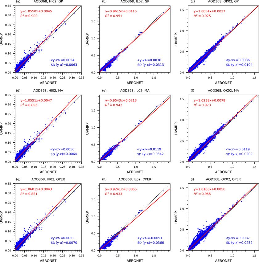
938                                         M. Chen et al.: Using GP regression to improve UV-MFRSR calibration factors

2.1.2    Proposed dynamic input uncertainty estimation              win_size of MA is set at 20 for all applicable cases in this
                                                                    study.
As mentioned before, the statistical properties of the noise
ε of the observedtime series y might be unknown. Even if          2.3   UVMRP operational algorithm (OPER)
assuming ε ∼ N 0, diag(σ 2y ) in practice, σ y is not always
a constant and could vary in time. Therefore, we propose to         UVMRP operational algorithm (OPER) was specially de-
estimate σ y with a moving window approach. Within each             signed for smoothing its in situ calibration factor sequences
moving window (W), the input uncertainty (denoted as si ) is        (http://uvb.nrel.colostate.edu/UVB/dataProcessingInfo/
assumed to be relatively stable and can be estimated using          VnaughtsDataProcessing.jsf, last access: 8 August 2018).
all points in the window (W). Note that si is not equivalent        OPER is included as an additional source for method
to the standard deviation of all points within the period (sW ),    comparison. The algorithm has three steps. In the first step, a
unless the mean function of the time series is invariant. We        12-count running mean and the corresponding standard de-
derive the relationship between si and sW (see Appendix A           viation are maintained to detect outliers (i.e., points outside
for the detailed derivation) to estimate si :                       half of the running mean or 2 standard deviations). During
                                                                    the process, if three consecutive points are determined to
                          J                                         be outliers, visual examination is performed to determine
 2      N −J 2      1 X                2
sW =         si +            Nj µj − µW ,                    (7)    if a permanent change in the instrument responsivity has
        N −1      N − 1 j =1
                                                                    occurred. If such a change is confirmed, calculation of a
where all points within W are clustered into J subgroups            new running mean begins on the three points. In the second
based on their similarity in both time and value; Nj is the         step, a moving linear regression (LR) is used to smooth the
number of points in each subgroup j ; N = Jj=1 Nj is the
                                                 P                  values at the center of each moving window. The moving
number of all points within W; µj is the mean of subgroup j ,       window size is ±3 months. If visual examination finds
which can vary among subgroups; si is the estimated uncer-          significant value changes on a date of interest (the center
tainty of each point within W, acting as the sample standard        of a moving window), the regression is not performed on
deviation across all subgroups; and µW and sW are the mean          that date. In the final step, the regression results from step
and sample standard deviation of all points within W. The           two are used as input into a weighted means algorithm to
classic K-means algorithm was used for the clustering pro-          generate continuous and smooth in situ calibration factors.
cess. To increase the reliability of estimating statistics (mean    The inverse of year fraction between the current date of
or sample standard deviation), small subgroups are merged           interest and the date of each participating point is used to
with adjacent ones to ensure each subgroup has more than            calculate the weights. The weighting window is also ±3
the required minimum points. The numbers of initial sub-            months from the date of interest.
groups and the required minimum points depend on the prior
knowledge of the variability and availability of the data. Sen-     2.4   Validation method for 368 nm in situ calibration
sitivity studies (not shown) indicate that five initial subgroups         factors
per moving window and three required minimum points per
subgroup worked well for our applications. The dynamic in-          Ideally, to avoid additional uncertainties caused by the
put uncertainty estimation process is applied to every data         interpolation among wavelengths, the calibration factors
point in a sequence. The squares of the estimated input stan-       should be validated via a direct comparison of direct
dard deviations (i.e., si2 in Eq. 7) are stored on the respective   sun signals from the to-be-calibrated UV-MFRSR and a
diagnostic positions in σ y .                                       reference instrument measuring at the 368 nm channel
   The flowchart of the proposed dynamic input uncertainty          (e.g., the standard precision filter radiometer (PFR) oper-
estimation method and the complete GP procedure of esti-            ated by the Physikalisches-Meteorologisches Observatorium
mating the mean and confidence interval functions of a given        Davos, World Optical Depth Research Calibration Center
time series is presented in Fig. 1.                                 (WORCC)). However, such reference measurements are not
                                                                    available at most UVMRP stations. Therefore, the estimated
2.2     Moving average (MA)                                         mean normalized V0 (V0,norm ) values from the GP regres-
                                                                    sion and the other two comparison methods (i.e., MA and
MA is a simple smoothing technique. To assess the per-              OPER) are validated indirectly in terms of aerosol opti-
formance of the GP regression with other methods, this              cal depth (AOD) against those obtained at the collocated
study implements MA for a one-dimensional case as fol-              AERONET sites. As shown in Appendix C, the uncertainty
lows. For a given x∗i , we first choose its nearby observa-         of UV-MFRSR AODs exceeds the World Meteorological Or-
tions {(x, y) ||x − x∗i | ≤ win_size, (x, y) ∈ Dobs } within the    ganization (WMO) U95 criterion (e.g., 95 % of the measured
given window win_size and then calculate the mean y value           data have uncertainty in the range of 0.005 ± 0.01 per air
of the subset as the smoothed observation at x∗i . The process      mass; Kazadzis et al., 2018) at the UVMRP sites investigated
is repeated for all possible x values in D∗ . The parameter         here because the stability assumption of the Langley method

Atmos. Meas. Tech., 12, 935–953, 2019                                                  www.atmos-meas-tech.net/12/935/2019/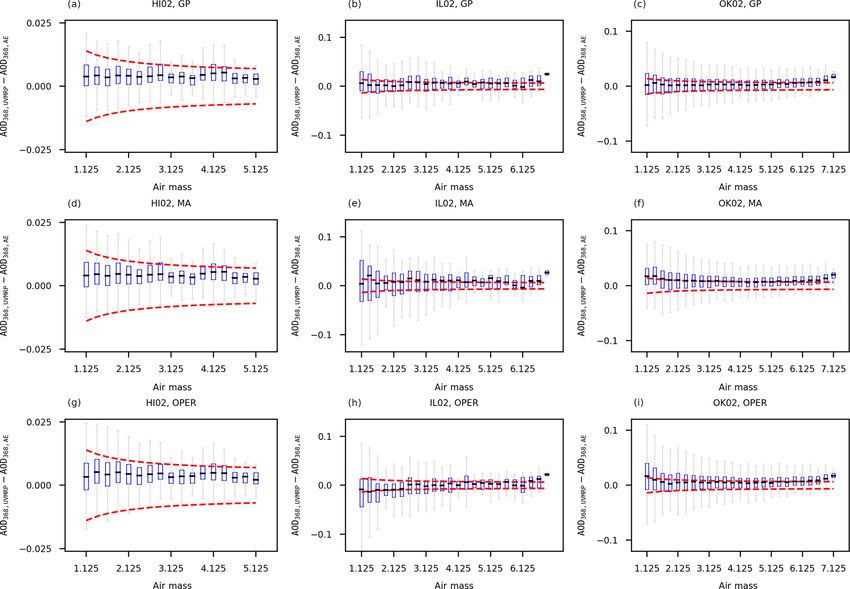
M. Chen et al.: Using GP regression to improve UV-MFRSR calibration factors                                                    939

Figure 1. Main procedure for deriving the mean and confidence interval functions using Gaussian process regression (a) and detailed
procedure of the proposed input uncertainty estimation method (b).

may not be strictly fulfilled. Therefore, the AOD compari-          Mountain station in Colorado with UVMRP MFRSR AODs
son in this study can only serve as indirect evidence to ver-       at the Pawnee station (85 km northeast of Table Mountain)
ify whether the calibration of UV-MFRSR is reasonably ac-           and with National Renewable Energy Laboratory (NREL)
curate. AERONET sun photometers are routinely calibrated            sun-photometer-derived AODs at Golden station (50 km to
with the uncertainty of AOD around 0.002 to 0.005 in the vis-       the south). The AOD difference in the test cases showed a
ible range and up to 0.01 in the UV region (Eck et al., 1999;       magnitude of 0.1 to 0.2 and was variable over time even
Holben et al., 2001) and are therefore considered a reliable        for the same comparison site. Krotkov et al. (2005a, b) vali-
source for AOD intercomparison and radiometer validation            dated the UVMRP UV-MFRSR AODs with the interpolated
(e.g., Alexandrov et al., 2002, 2008; Augustine et al., 2003;       AERONET AODs at the 368 nm at the National Aeronau-
Krotkov et al., 2005a, b; Kassianov et al., 2007; Tang et al.,      tics and Space Administration Goddard Space Flight Center
2013; Yin et al., 2015; Zhang et al., 2016). During the recent      (NASA/GSFC) site in Greenbelt, Maryland. They found that
Fourth WMO Filter Radiometer Comparison held in Davos,              the UV-MFRSR AODs at 368 nm channel on cloud-free days
Switzerland (between 28 September and 16 October 2015),             had a daily RMSE of less than 0.01 when calibrated using
most AOD values derived from the three AERONET CIMEL                AERONET measurements and increased to approximately
sun photometers are within the ±0.01 range compared with            0.02–0.05 (depending on the season) when calibrated using
the PFR triad standard (Kazadzis et al., 2018). This in-            the standard Langley method (Harrison and Michalsky, 1994;
cludes those determined at 368 nm from the extrapolation of         Slusser et al., 2000). Alexandrov et al. (2002) developed
AERONET AODs at 340 and 380 nm. The 2015 Davos cam-                 a comprehensive calibration method for the VIS-MFRSR
paign also included four MFRSR instruments. Overall, the            and validated the calibration at the four channels (i.e., 440,
results showed good agreement among the four MFRSRs and             500, 670, and 870 nm) by comparing the derived AOD val-
the PFR triad standard, though one instrument exhibited a           ues with interpolated AERONET values at the ARM Cloud
positive bias and low precision compared to the sun-pointing        and Radiation Testbed (CART) site. The results showed a
instruments (Kazadzis et al., 2018). However, such errors           small AOD difference (i.e., < 0.005) at the 440, 500, and
were likely explained by instrument-specific uncertainties          870 nm channels for a variety of atmospheric conditions with
(e.g., angular response correction, responsivity calibration,       AODs ranging from 0.03 to 0.4 (at 500 nm). Alexandrov et
and shadowband position issues) and do not suggest inherent         al. (2008) considered optical depth of NO2 and ozone dur-
error in MFRSR AODs (Kazadzis et al., 2018). Augustine et           ing the MFRSR AOD calculation, although they were small
al. (2003) compared SURFRAD MFRSR AODs at the Table                 enough to be ignored (i.e., 0.008 NO2 optical depth at 415 nm

www.atmos-meas-tech.net/12/935/2019/                                                    Atmos. Meas. Tech., 12, 935–953, 2019
940                                        M. Chen et al.: Using GP regression to improve UV-MFRSR calibration factors

and 0.005 ozone optical depth at 615 nm) at their test lo-        log(wavelength)), log(AOD) is generally linear between 340
cation at the ARM Southern Great Plains (SGP) site. The           and 380 nm (Krotkov et al., 2005a). First, the AERONET
long-term intercomparison showed a good agreement (i.e.,          AOD spectrum between the two wavelengths is derived by
difference between them < 0.01) between the MFRSR and             linear interpolation of AERONET AODs at 340 and 380 nm
AERONET AODs at the 440, 675, and 870 nm channels.                in the log-transformed coordinate system. Next, since the
Kassianov et al. (2007) validated the MFRSR-retrieved opti-       UV-MFRSR AOD at 368 nm is a band-pass value over a nar-
cal properties and reported small RMSE values (i.e., 0.0043–      row band (i.e 2 nm FHMW), the equivalent AERONET AOD
0.0075) among MFRSR, AERONET, and normal incidence                at that channel is derived by
multifilter radiometer (NIMFR) AODs at the 500 and 870 nm
                                                                                          R 380 nm
channels during the ARM program’s Aerosol Intensive Op-
                                                                                           340 nm AODλ Fλ dλ
erational Period (IOP) in 2003.                                   AOD368 nm,AERONET =        R 380 nm        ,               (9)
   In this study, for the UV-MFRSR at the 368 nm chan-                                         340 nm Fλ dλ
nel, AOD (AOD368 nm,UVMRP ) is calculated by subtracting
Rayleigh optical depth (RLOD368 nm,UVMRP ) from total op-         where AODλ is the interpolated AERONET AOD spectrum,
tical depth (TOD368nm,UVMRP ) under cloud-free conditions.        Fλ is the spectral response function of the UV-MFRSR at
The absorption of O3 , NO2 , and other trace gases is very        the 368 nm channel (http://uvb.nrel.colostate.edu/UVB/da_
small at the 368 nm channel (e.g., NO2 optical depth is           queryFilterFunctions.jsf, last access: 8 August 2018), and the
around 0.002 to 0.003 at AERONET Cart_Site), so they are          wavelength interval for the integral is 0.05 nm. Note that neg-
ignored during the calculation of AOD368 nm,UVMRP :               ative AERONET AOD measurements are excluded from the
                                                                  validation because of using log transformation.
AOD368 nm,UVMRP ≈ TOD368 nm,UVMRP                                    Since AERONET and UV-MFRSR AOD values at 368 nm
                                                                  are derived from measurements involving different instru-
   − RLOD368 nm,UVMRP .                                    (8)
                                                                  ments and wavelengths, the uncertainties when comparing
TOD is calculated using Beer’s law (e.g., Slusser et al.,         these AOD values should be noted. Some important sources
2000), for which the actual calibration factor at the top         of uncertainties include the following.
of the atmosphere (V0,raw ) is restored from GP-estimated
                                                                   1. AERONET calibration error. At the time of calibra-
mean V0,norm . The cosine-corrected voltage and air mass
                                                                      tion at Mauna Loa Observatory, AERONET reference
are obtained from the UVMRP web page (https://uvb.
                                                                      instruments have an uncertainty of ∼ 0.2 % to 0.5 %,
nrel.colostate.edu/UVB/da_queryCosCorrected.jsf, last ac-
                                                                      which is equivalent to a 0.002 to 0.005 uncertainty in
cess: 8 August 2018). RLOD is calculated by following the
                                                                      AERONET AOD (Holben et al., 2001). These calibra-
equations in Bodhaine et al. (1999). The site latitude and
                                                                      tion factors are likely to shift within the year following
height for RLOD calculation are from the UVMRP web page
                                                                      calibration, which may result in a total AOD uncertainty
(https://uvb.nrel.colostate.edu/UVB/uvb-siteinfo.jsf, last ac-
                                                                      of ∼ 0.01 to 0.02 (wavelength dependent, higher in the
cess: 8 August 2018), and the instantaneous site-level sur-
                                                                      UV) (Holben et al., 2001).
face pressure for RLOD calculation is obtained from the
collocated AERONET sites (https://aeronet.gsfc.nasa.gov/
cgi-bin/webtool_opera_v2_new, last access: 31 July 2018).          2. Instrument field of view (FOV). AERONET CIMELs
   To obtain reliable AOD values, UV-MFRSR measure-                   have a FOV of 1.2◦ while the UV-MFRSR has a larger
ments with quality concerns or cloud contamination are                FOV (e.g., ∼ 6.5◦ ; reported by Kazadzis et al., 2018).
excluded in the following comparison. More specifically,              AODs obtained from instruments with larger FOVs are
(1) any measurements with UVMRP-provided quality con-                 associated with greater AOD uncertainty due to larger
trol flag(s) relevant to the data quality of the direct beam at       contributions of scattered light to the direct irradiance
the 368 nm channel are excluded; (2) data with small (direct          measurement (Kim et al., 2005).
beam) measurements at 368 nm are also excluded because
they are more sensitive to noise or errors introduced during       3. Instrument maintenance. Periodic soiling and cleaning
various calibration steps; and (3) a simple variation check is        of the UV-MFRSR diffuser can result in spurious in-
performed to reduce the potential of mixing cloud and AOD.            creases and decreases in AOD, respectively. The fre-
If the ratio between the standard deviation of TODs and the           quency of on-site maintenance (e.g., cleaning of the UV-
mean TOD value in the 15 min time window exceeds 0.05,                MFRSR dome) as well as rainfall events may therefore
they are excluded from further analyses.                              account for some of the AOD difference (Kim et al.,
   AERONET (v2.0) provides AOD at the 340 and 380 nm                  2005, 2008).
channels. These values are interpolated to the effective wave-
length of the UV-MFRSR 368 nm channel for compari-                 4. Trace gases. As mentioned above, AERONET AOD ac-
son using the Ångström exponent as follows. Note that in              counts for NO2 optical depth (e.g., ∼ 0.002–0.003 at
the log-transformed coordinate system (i.e., log(AOD) vs.             OK02) while UV-MFRSR AOD does not.

Atmos. Meas. Tech., 12, 935–953, 2019                                                www.atmos-meas-tech.net/12/935/2019/
M. Chen et al.: Using GP regression to improve UV-MFRSR calibration factors 941
2.5 Datasets
2.5.1 Synthetic case
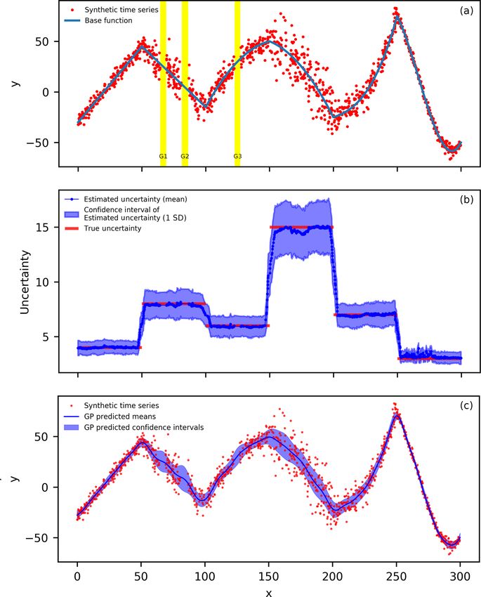
We generate a synthetic time series that is composed of
six segments with a varying base function and noise lev-
els (Fig. 2a). The base function (Eq. 10), including linear,
quadratic, and cubic functions, simulates a wide variety of
functions for which the proposed technique is applicable.
The noise levels are the same within each segment but differ-
ent across segments. The noise at segment i is sampled from
a fixed normal distribution N 0, σi2 , where σi is equal to 4,
8, 6, 15, 7, and 3 from left to right segments. Each segment
originally contains 200 points. Their x coordinates are sam-
pled randomly from six uniform distributions within their do-
mains. Points with x coordinates in the three designated win-
dows (i.e., [64.2, 69.2], [80.8, 85.8], and [122.5, 127.5]) are
removed to simulate data gaps in reality.
1.5x − 30, 0 ≤ x < 50
−1.2(x − 50) + 45, 50 ≤ x < 100
−0.02(x − 100)2
100 ≤ x < 150
+2.3(x − 100) − 15,
−0.02(x − 150)2
150 ≤ x < 200
−0.5(x − 150) + 50,
y= (10)
0.0004(x − 200)3 200 ≤ x < 250
+0.012(x − 200)2 Figure 2. (a) The synthetic time series based on Eq. (10) (the blue
+0.4(x − 200) − 25, line) with varying noise levels. There are originally 200 samples
0.002(x − 250)3 250 ≤ x < 300 within every 50-wide interval (or segment) in the x coordinate, but
−0.1(x − 250)2 points between [64.2, 69.2] (highlighted in yellow, G1), [80.8, 85.8]
(highlighted in yellow, G2), and [122.5, 127.5] (highlighted in yel-
−2.5(x − 250) + 75,
low, G3) are removed to simulate data gaps in practice. The final
number of points in the sequence is 1140. (b) The means (dark blue
2.5.2 Application cases: in situ calibration factors circles) and confidence intervals (light blue area) of the estimated
uncertainty for the 200 synthetic sequences (all sampled from the
In this study, the in situ calibration factors of UVMRP UV- distribution of (a) but with different random noise). The true uncer-
MFRSRs are used as application cases to test the perfor- tainty (red line segments) is also displayed. (c) The Gaussian pro-
mance of the three smoothing methods (i.e., GP, MA, and cess regression results for the synthetic time series from (a). The
OPER). These UV-MFRSR in situ calibration factors over dark blue line is the predicted mean function and the light blue area
several months or years are obtained through the Lang- is the corresponding confidence intervals.
ley method on clear days. Their varying uncertainties are
mainly attributed to two aspects. One is the optical stabil-
ity of atmospheric constituents (e.g., the aerosol, ozone, and show that the UV-MFRSR 368 nm in situ calibration factors
thin clouds) when the in situ calibration factor is derived obey normal distribution.
(Chen et al., 2015), and the other is the aging status of
the radiometer. UVMRP publish its in situ calibration fac-
3 Results and discussion
tors on their website (http://uvb.nrel.colostate.edu/UVB/da_
queryVoIntercepts.jsf, last access: 8 August 2018). To re- 3.1 Synthetic case
duce the chances of abrupt changes in the sequences, the
data associated with the same instrument (i.e., UV-MFRSR) 3.1.1 Estimation of input uncertainty for Gaussian
at the same UVMRP site (denoted as a deployment period) process
are processed together. Three UVMRP sites with collocated
AERONET sites (for validation) were selected (Table 1). The The proposed dynamic input uncertainty estimation method
in situ calibration factors at these UVMRP sites represent is first applied to the synthetic case. To observe the statisti-
time series with contrasting densities, noisiness, and slopes cal properties and characteristics of the estimated input un-
(Table 1). Appendix B uses the Oklahoma site (OK02) to certainty, this procedure was applied to 200 synthetic time
www.atmos-meas-tech.net/12/935/2019/ Atmos. Meas. Tech., 12, 935–953, 2019942 M. Chen et al.: Using GP regression to improve UV-MFRSR calibration factors
Table 1. The three UVMRP 368 nm UV-MFRSR in situ calibration factor time series for test.
UVMRP site UVMRP site location Collocated AERONET Deployment start and end dates Figure (original Time series characteristics
name site time series)
HI02 19.54◦ N, 155.58◦ W, 3409 m Mauna_Loa 17 September 2015 to 1 July 2018 Fig. 3a1 dense, low noise, variable slope
IL02 40.05◦ N, 88.37◦ W, 213 m BONDVILLE 21 March 2017 to 29 May 2018 Fig. 3b1 sparse, high noise, sharper slope
OK02 36.60◦ N, 97.49◦ W, 317 m Cart_Site 17 January 2007 to 11 June 2011 Fig. 3c1 medium density, medium noise,
variable slope
series, each of which is generated by adding random noise we round the original data points (red points in Fig. 2a) to the
into the base function (Eq. 10) following the procedures dis- nearest 0.25 interval grids. Then, we calculate the autocorre-
cussed in Sect. 2.5.1. lation on these rounded data points from lags of 0.25 to 22.25
Figure 2b shows the means (dark blue circles) and con- (approximately equivalent to lags of 1 to 90 points). Next,
fidence intervals (light blue area) of estimated uncertainty we perform curve fitting on autocorrelation results and ob-
of the 200 estimated input uncertainty sequences. The mean tain 9.80 and 1.05 as initial length scale and alpha estimates,
of the estimated uncertainty is close to the true uncertainty respectively. With these initial RQ parameters and the esti-
(RMSE = 0.6321) for the entire synthetic case as demon- mated input uncertainty (from the proposed method or using
strated by a LR between estimated and true uncertainty with three representative constant input uncertainties), GP regres-
a slope close to 1 (i.e., 1.0332) and a high R 2 of 0.9759 sion predicts the mean and uncertainty functions. Figure 2c
(Table 2). Most true uncertainty (red line segments) is cov- shows the GP results for the proposed method: dark blue line
ered by the confidence intervals except for the areas near the for the mean function and the light blue area for the confi-
ends of the six segments. In these areas, the method averaged dence intervals (4.42 times of the GP-predicted uncertainty
the uncertainty from the adjacent segments and presented function).
a smooth transition between segments. This small RMSE In terms of the GP-predicted mean function vs. the base
value suggests that using smaller subgroup size (e.g., three to function (Eq. 10), the proposed input uncertainty estimation
six points) does not significantly influence the estimation of method shows a 12.0 % to 15.7 % improvement on RMSE
uncertainty (Fig. 2a). Therefore, smaller subgroups are pre- over the three constant input uncertainties (i.e., 1.1785 vs.
ferred over larger ones as larger subgroups are more likely to 1.3146, 1.3976, and 1.3146) (Table 2). Similarly, the slope
have gap(s) with large variation, which tends to increase its of the LR between the two functions is closer to 1 for the
estimated standard deviation (Eq. 7). proposed uncertainty estimation method (i.e., 1.0082) than
To demonstrate the improvements in the GP resulting from the three constant uncertainties (i.e., 1.0228). In addition, the
the dynamic input uncertainty estimation, the GP is also run predicted mean function from the proposed method is close
with three typical constant input uncertainties: overall stan- to the base function even near the gaps (G1, G2, and G3 in
dard deviation of the synthetic time series (30.95), minimum Fig. 2a, c). Additionally, the proposed method’s predicted
true uncertainty of the synthetic time series (2.00), and max- uncertainty function (or confidence intervals) shows better
imum true uncertainty of the synthetic time series (15.00). agreement with the true uncertainty of the synthetic time se-
The results from all three constant input uncertainties are ries (Fig. 2c) while the three constant input uncertainties’ re-
less accurate than the estimated input uncertainty generated sults show a consistent over- or underestimated pattern over
by the proposed method (Table 2). The proposed method has the entire time series (figures not shown). It is noted that the
a significantly smaller RMSE (i.e., 0.6321) compared with predicted confidence intervals from the proposed method are
the three constant input uncertainties (i.e., 24.1152, 6.5226, wider near the three gaps (G1, G2, and G3 in Fig. 2a) than
and 8.7921, respectively). Similarly, the LR between the esti- nearby locations with similar uncertainty. This is anticipated
mated and true uncertainties shows that the proposed method because the constraint in the gaps are from distant points at
has slope and R 2 values both close to 1 (i.e., 1.0332 and which the RQ kernel gives low correlation.
0.9759) while the three constant uncertainties show no (lin-
ear) correlation with true uncertainties (i.e., the slope and R 2 3.2 In situ calibration factors cases
values close to zero).
3.2.1 Applications
3.1.2 Estimation of means and confidence interval and
its validation The same GP procedure is applied to three in situ cali-
bration factor (V0,norm , sun-earth distance normalized) se-
The kernel function in the GP regression used in this study is quences from three UVMRP deployment periods (Fig. 3) at
the RQ kernel, with two parameters: length scale and alpha three different UVMRP locations previously described in Ta-
(Eq. 2). To use RQ with GP regression, we need to provide ble 1.The Hawaii site (HI02) sits at a clean, high-altitude lo-
the initial (estimated) values for these two parameters. First, cation, which means its atmospheric condition is more stable
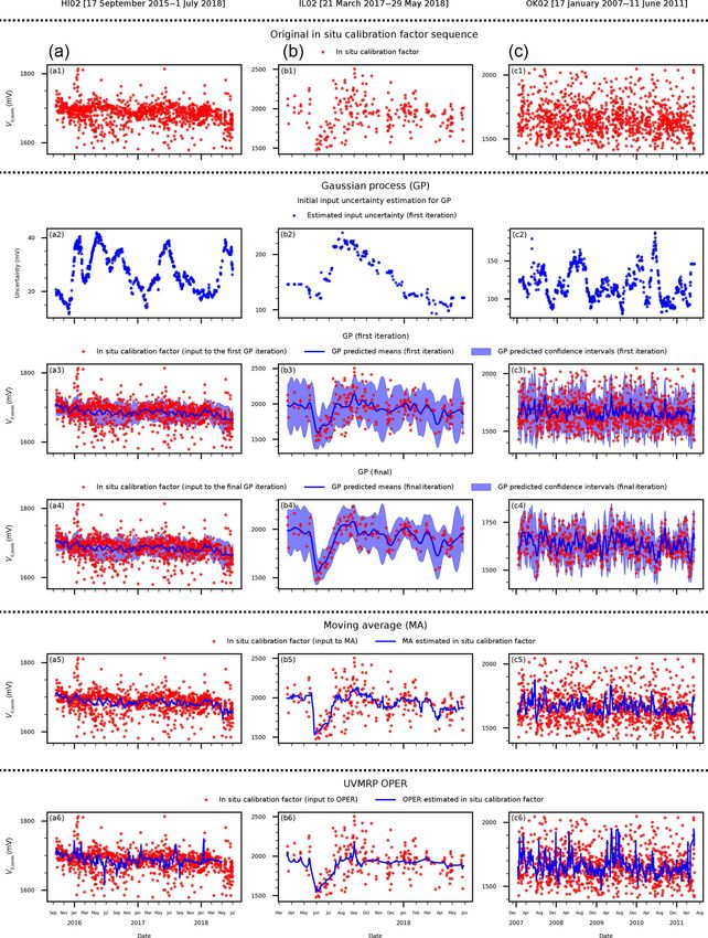
Atmos. Meas. Tech., 12, 935–953, 2019 www.atmos-meas-tech.net/12/935/2019/M. Chen et al.: Using GP regression to improve UV-MFRSR calibration factors 943 Figure 3. The results of the three smoothing methods (i.e., GP – Gaussian process; MA – moving average; OPER – UVMRP operational algorithm) for the three UVMRP in situ calibration factor sequences: (a) HI02 (17 September 2015 to 1 July 2018), (b) IL02 (21 March 2017 to 29 May 2018), and (c) OK02 (17 January 2007 to 11 June 2011). Panels (a1), (b1), (c1) display the original in situ calibration factor (V0,norm ) sequence. Panels (a2), (b2), (c2) show the initial input uncertainty estimated for GP. Panels (a3), (b3), (c3) present the predicted daily mean and confidence interval from the first iteration of GP. Panels (a4), (b4), (c4) show the final results of GP after iterations. Panels (a5), (b5), (c5) show the results of MA. Panels (a6), (b6), (c6) show the results of OPER. www.atmos-meas-tech.net/12/935/2019/ Atmos. Meas. Tech., 12, 935–953, 2019
944 M. Chen et al.: Using GP regression to improve UV-MFRSR calibration factors
GP-estimated mean values using the respective input uncertainty.
than other UVMRP sites and its V0,norm has the lowest varia-
Note: 1 y1 represents the true input uncertainty of the synthetic time series; x1 represents the estimated input uncertainties. 2 y2 represents the true values on the base function (Eq. 10); x2 represents the
RMSE stands for root-mean-square error. LR stands for linear regression. R 2 stands for the coefficient of determination for linear regression.
standard deviation of the synthetic time series (30.95), minimum true uncertainty of the synthetic time series (2.00), and maximum true uncertainty of the synthetic time series (15.00).
Table 2. Validation of the input uncertainty and mean of GP prediction using four input uncertainties: the input uncertainty estimated by the proposed method (Sect. 2.1.2), overall
Mean of GP prediction
Input uncertainty
tion (Fig. 3a1). The Illinois site (IL02) is surrounded by crop-
lands/rangelands with the closest city (Champaign) located
12 km northwest (Fig. 3b1). The Oklahoma site (OK02) is
also surrounded by croplands/rangelands with the closest city
(Oklahoma City) located about 96 km south (Fig. 3c1). Both
wildfires and agricultural activities (e.g., cultivation and har-
vest) at IL02 and OK02 contribute to the relatively hazy and
unstable atmosphere condition for Langley regression. As a
R2
LR2
RMSE
R2
LR1
RMSE
Metrics
result, V0,norm values at IL02 and OK02 have larger vari-
ation compared with HI02. The dynamic input uncertainty
estimation results confirm that the uncertainty at HI02 (15–
Proposed input uncertainty
40; Fig. 3a2) is also lower than at the other two sites (100–
y2 = 1.0082x2 − 0.3865
y1 = 1.0332x1 − 0.2277
300; Fig. 3b2, c2). Generally, the proposed method gives
lower uncertainty values for time windows with more clus-
estimation method
tered points (e.g., December 2008 and April 2010 at OK02,
Fig. 3c2; February 2017 at HI02, Fig. 3a2). There are no
obvious temporal patterns of uncertainty at any of the three
0.9986
1.1785
0.9759
0.6321
sites.
Figure 3a3, b3, and c3 show the estimated means (dark
blue line) and confidence intervals (light blue area) after the
y1 = −0.1962x1 − 0.2277
Overall standard deviation
initial pass through GP. The length scale parameters of the
y2 = 1.0228x2 − 0.5351
RQ kernel for the HI02, IL02, and OK02 sites are 6.091,
6.369, and 6.228 (days), respectively. Their corresponding
alpha parameters of the RQ kernel function are all close to
1.0 (i.e., 0.948, 0.862, and 0.944, respectively). As expected,
the confidence interval is narrower near time windows with
24.1152
(30.95)
0.9986
1.3146
more data points, and the confidence intervals are wider near
0.0
gaps (Fig. 3b3).
As depicted in Fig. 1, the outlier removal and GP are re-
Minimum synthetic time series
peated following the initial GP regression, giving the final GP
results shown in Fig. 3a4, b4, and c4. After this final pass,
Constant input uncertainty
y2 = 1.0228x2 − 0.5636
the length scale parameters of the RQ kernel function for
y1 = 0.0x1 + 7.1632
the HI02, IL02, and OK02 sites are 6.091, 11.149, and 6.907
uncertainty (2.00)
(days), respectively. Compared with the first round, all length
scale parameters increase as more outliers are removed (ex-
cept for HI02). At HI02, the average ratio between GP means
and standard deviations is lower than the threshold (i.e., 0.01)
0.9983
1.3976
6.5226
after the first round and the iteration stops. The correspond-
0.0
ing alpha parameters of the RQ kernel function are still all
close to 1.0 (i.e., 0.948, 1.010, and 1.110, respectively). Be-
Maximum synthetic time series
cause of outlier removal, compared with the first-round re-
sults, GP generates smoother mean functions and narrower
y2 = 1.0228x2 − 0.5351
confidence intervals at the last round.
y1 = 0.0x1 + 7.1632
uncertainty (15.00)
The other two methods (i.e., MA and OPER) are applied
to the same in situ calibration time series. They can pro-
vide mean functions but not confidence intervals. The MA
(win_size = 20) results (Fig. 3a5, b5, and c5) are generally
0.9986
1.3146
8.7921
smoother than OPER (Fig. 3a6, b6, and c6) but both are more
0.0
responsive to noisy points than GP. In addition, since OPER
is scheduled to run once per month on active deployments,
there may be some lags at the end of those deployments (e.g.,
Fig. 3a6).
Atmos. Meas. Tech., 12, 935–953, 2019 www.atmos-meas-tech.net/12/935/2019/M. Chen et al.: Using GP regression to improve UV-MFRSR calibration factors 945
Figure 4. The 368 nm AOD scatter plots between UVMRP (y axis) and AERONET (x axis). The UVMRP 368 nm AODs are calculated
from UV-MFRSR direct normal voltages using calibration factors estimated by the three methods (i.e., from top to bottom: GP, MA, OPER)
at the three sites (i.e., from left to right: HI02, IL02, OK02). Panels (a), (b), and (c) display the scatter plots for the GP method at HI02,
IL02, and Ok02, respectively. Similarly, panels (c), (c), and (f) are for the MA method and panels (g), (h), and (i) are for the OPER method.
The AERONET 368 nm AODs are derived from collocated (i.e., Mauna_Loa, BONDVILLE, Cart_Site) AERONET AODs on the 340 and
380 nm channels. The linear regression line (solid, red) and the 1-by-1 line (dashed, black) are also plotted. “< y − x >” means the average
difference between AERONET and UVMRP AOD at the 368 nm channel. “SD(y − x)” means the standard deviation of their difference.
3.2.2 Validation (Fig. 4a, d, g) are similar. For example, the average bias
“< y − x >” is approximately 0.0054 and standard deviation
of the difference “SD(y − x)” is approximately 0.0066. For
Following the procedures described in Sect. 2.4, the UVMRP IL02 (Fig. 4b, e, h) and OK02 (Fig. 4c, f, i), GP shows su-
AODs at the 368 nm channel generated by GP, MA, and perior agreements with AERONET to that of the other two
OPER are validated against the corresponding AERONET methods. For example, at IL02, the absolute value of GP’s
AODs at the three collocated sites (i.e., HI02 – Mauna_Loa, average bias (0.0036) is about 3.3 to 2.5 times lower than that
IL02 – BONDVILLE, OK02 – Cart_ Site). The scatter plots of MA (0.0119) and OPER (0.0091). Similarly, at OK02, the
between these UVMRP and AERONET AODs are displayed average bias for GP (0.0032) is much lower than that for MA
in Fig. 4. The performance of all three methods at HI02
www.atmos-meas-tech.net/12/935/2019/ Atmos. Meas. Tech., 12, 935–953, 2019946 M. Chen et al.: Using GP regression to improve UV-MFRSR calibration factors
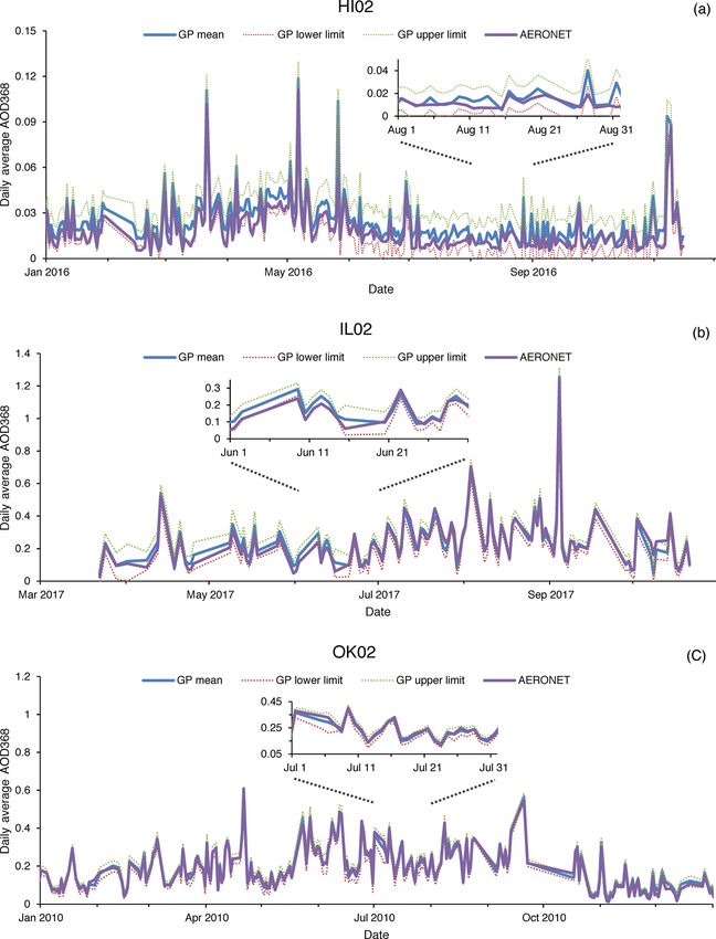
Figure 5. Time series of UVMRP and AERONET 368 nm daily average AOD at the HI02, IL02, and OK02 sites. The daily AOD mean
values derived from the GP mean in situ calibration factor (V0 ) functions (blue) and the corresponding AERONET values (purple) are shown
as solid blue lines. The corresponding lower and upper limits of AOD derived from the GP V0 confidence intervals are shown as dotted red
and green lines, respectively. The insets for HI02 (August 2016), IL02 (June 2017), and OK02 (July 2010) are also included in the respective
subplots to show the comparison details.
(0.0119) and OPER (0.0087). The validation results for GP at Table 3 shows two additional statistical metrics for val-
OK02 are similar to the previous comparison results between idation: “Avg(|AOD368,UVMRP − AOD368,AE |)”, a measure
AERONET and MFRSR AODs at 415 and 440 nm (Tang et of absolute difference between the two quantities and
al., 2013; Alexandrov et al., 2008). Furthermore, as shown “Avg(|AOD368,UVMRP − AOD368,AE |/AOD368,AE )” a mea-
in Appendix C, the GP method improves agreement between sure of relative difference between the two quantities. For
UVMRP and AERONET 368 nm AOD across all air masses. HI02, the GP V0,norm values improve both the absolute and
relative differences between AOD368,UVMRP and AOD368,AE
Atmos. Meas. Tech., 12, 935–953, 2019 www.atmos-meas-tech.net/12/935/2019/M. Chen et al.: Using GP regression to improve UV-MFRSR calibration factors 947
Table 3. Statistical metrics (average absolute difference, average absolute relative difference, and linear regression) on comparing 368 nm
AOD between UVMRP (AOD368,UVMRP ) and AERONET (AOD368,AE ). The UVMRP 368 nm AODs at the three sites (i.e., HI02, IL02,
and OK02) are calculated using calibration factors estimated using the three methods (i.e., GP, MA, and OPER). The AERONET 368 nm
AODs are derived from collocated (i.e., Mauna_Loa, BONDVILLE, and Cart_Site) AERONET AODs on the 340 and 380 nm channels. LR
stands for linear regression. R 2 stands for the coefficient of determination for linear regression. The “x” and “y” in LR refer to AOD368,AE
and AOD368,UVMRP of the respective methods.
Method
Site Metrics
GP MA OPER
Avg|AOD368,UVMRP − AOD368,AE | 0.0062 0.0065 0.0067
|AOD368,UVMRP −AOD368,AE |
HI02 Avg AOD 0.5803 0.6078 0.6261
368,AE
LR y = 1.0550x + 0.0045 y = 1.0551x + 0.0047 y = 1.0601x + 0.0043
R2 0.9000 0.8957 0.8812
Avg(|AOD 368,UVMRP − AOD368,AE |) 0.0228 0.0291 0.0270
|AOD368,UVMRP −AOD368,AE |
IL02 Avg AOD 0.1669 0.2087 0.1930
368,AE
LR y = 0.9615x + 0.0115 y = 0.9543x + 0.0213 y = 0.9241x + 0.0065
R2 0.9514 0.9420 0.9332
Avg|AOD368,UVMRP − AOD368,AE | 0.0150 0.01785 0.01847
|AOD368,UVMRP −AOD368,AE |
OK02 Avg AOD 0.1714 0.2067 0.1939
368,AE
LR y = 1.0054x + 0.0027 y = 1.0238x + 0.0078 y = 1.0186x + 0.0056
R2 0.9749 0.9726 0.9554
when compared to MA (by ∼ 4.5 %) and OPER AODs (by In addition, Fig. 5 shows the 368 nm AOD time series
∼ 7.5 %), respectively. Results from LRs performed between calculated using GP-generated in situ calibration factors at
AOD368,UVMRP and AOD368,AE are also reported in Table 3. the three UVMRP sites. The blue solid line represents the
The LR results are similar between GP and MA, but GP has AODs calculated using the GP means, and the green and
a LR slope closer to 1 (1.0550) and higher R 2 (0.9000) than red dotted lines represent the AODs calculated using the GP
those of OPER (1.0601 and 0.8812) for HI02. For IL02, GP confidence intervals. It is seen that the AOD confidence in-
shows 21.6 % smaller absolute difference and 20.0 % smaller tervals are approximately ±0.0095, ±0.0480, and ±0.0273
relative difference to AERONET than MA; GP shows 15.6 % at HI02, IL02, and OK02, respectively. The corresponding
smaller absolute difference and 13.5 % smaller relative dif- AERONET AOD time series are also plotted (i.e., purple
ference to AERONET than OPER. Similarly, for OK02, GP lines in Fig. 5). The insets in Figure 5 show comparison
shows 16.0 % smaller absolute difference and 17.1 % smaller details at HI02, IL02, and OK02. For most of the AOD
relative difference to AERONET than MA; GP shows 18.8 % time series, AERONET results are within the GP confi-
smaller absolute difference and 11.6 % smaller relative dif- dence intervals. The average absolute differences of daily
ference to AERONET than OPER. AOD values between GP and AERONET are ∼ 0.006 for
Overall, the 368 nm AODs by GP show higher correla- HI02, ∼ 0.024 for IL02, and ∼ 0.014 for OK02. These val-
tion, closer to 1 slopes, and lower absolute and relative bi- ues are close to or within the AERONET AOD uncertainty
ases compared to AERONET AODs than MA and OPER at level (i.e., 0.01), suggesting the high quality of the poten-
all three sites. The improvement of GP over MA and OPER tial UVMRP AOD product. In addition, unlike the obvious
at IL02 and OK02 is more significant than at HI02. The main seasonal changes in AOD difference reported in the previous
reason may be that HI02 is the least polluted site among the study at the NASA/GSFC site by Krotkov et al. (2005a), this
three sites. Both of its maximum and mean 368 nm AOD val- study (Fig. 5) shows no discernible seasonal pattern in the
ues are low: 0.35 and 0.016, respectively. As a result, higher AOD differences at all three sites.
accuracy of Rayleigh and other optical depth components is
required to discern small improvement in AOD for HI02.
Since AERONET’s sun photometer is routinely calibrated, 4 Conclusions
the agreement on AOD values suggests that the calibration
factor mean functions generated by GP are more accurate A new dynamic uncertainty estimation method for noisy time
than those of MA and OPER. series is developed in this study. Combining this method
with Gaussian process regression, we provide a solution to
estimate the underlying mean and uncertainty functions of
www.atmos-meas-tech.net/12/935/2019/ Atmos. Meas. Tech., 12, 935–953, 2019948 M. Chen et al.: Using GP regression to improve UV-MFRSR calibration factors time series with variable mean, noise, sampling density, and length of gaps. For the synthetic case with linear, quadratic, and cubic base functions; a noise level varying from 2 to 15; and noticeable gaps, the proposed solution returns a mean function with the RMSE of 1.1785 (linear regression R 2 of 0.9986), which is at least 12.0 % lower than RMSEs associ- ated with the three constant input uncertainties. Its estimated input uncertainties determined by this method are close to the true uncertainty levels except for the transitional region between segments. The solution also gives accurate mean values at the three gaps. The proposed GP solution as well as the other two comparison methods (i.e., MA and OPER) were then applied to three in situ calibration factor time se- ries of UV-MFRSR (368 nm) at three UVMRP sites. The GP solution handles the variation in slope, noise, sampling den- sity, and length of gap in the three cases as expected. Since irradiance at 368 nm is not measured by a collocated (and calibrated) radiometer, the performance of the three methods is validated against the collocated AERONET sites in terms of AOD. The results show that AODs calculated using GP- derived UV-MFRSR calibration factors (V0,norm ) have con- sistently better agreement with AERONET AODs than MA and OPER in terms of average absolute and relative differ- ences and linear regression R 2 values. These results suggest that the proposed GP solution is a robust method for time series analyses of data with variable mean, noise, sampling density, and length of gap and has potential for application across disciplines. Atmos. Meas. Tech., 12, 935–953, 2019 www.atmos-meas-tech.net/12/935/2019/
M. Chen et al.: Using GP regression to improve UV-MFRSR calibration factors                                                            949

Appendix A: The formulation between the overall                            Appendix B: The distribution of the 368 nm in situ
standard deviation and the subgroup standard deviation                     calibration factors of UV-MFRSR

Given a time series {xi }, its total N points are divided into             Since the true 368 nm in situ calibration factors are not
                j
J groups {xk }, and the number of points in group j is Nj                  available, their distribution is derived using the AERONET
(j = 1, 2, . . . , J ; k = 1, 2, . . . , Nj ). For data points in each     368 nm AOD distribution via Beer’s law (transformed Lang-
group, their sample mean and standard deviation are µj and                 ley regression).
                                                                 N            Beer’s law links the irradiance (or voltage, V ) at the top of
sj . For the entire time series, its sample mean is µ = N1
                                                                 P
                                                                    xi ,   the atmosphere with the one that reaches the ground at time
                                                                i=1
and the sample variance is                                                 t with the equation Vt = V0 e−TODt ·mt , where mt is the air
                                                                           mass at time t and TODt is the corresponding total optical
               J X Nj                                                      depth. For the 368 nm channel, AOD is the main contribu-
         1 X            j
s2 =                  (x − µ)2                                             tor for the TOD variation. Therefore, for a short time period,
       N − 1 j =1 k=1 k
                                                                           TODt can be expressed as the sum of a constant optical depth
               J X Nj                                                      (P ) and variable residual AOD (1AODt = AODt − AOD):
         1 X             j
   =                  [(x − µj ) + (µj − µ)]2                              TODt = P + 1AODt . Deriving an unbiased V0 using the
       N − 1 j =1 k=1 k                                                    Langley regression (in the transformed lnV · m−1 vs. m−1
             J X Nj                     J X Nj                             coordinate system) requires the participating measurements
       1 X            j      2    1 X
   =                (x − µj ) +                (µj − µ)2                   to have a constant TODt over the calibration period and lnV0
     N − 1 j =1 k=1 k           N − 1 j =1 k=1                             is the slope of the regression. The variation in 1AODt as
               J X Nj                                                      a linear function of the component vary linearly with m−1     t
         2 X            j                                                  (Chen et al., 2014). Therefore, we decompose 1AODt as the
   +                  (x − µj )(µj − µ)
       N − 1 j =1 k=1 k                                                    sum of a constant term (α) and a m−1                 −1
                                                                                                                  t term (βmt ), where
               J                   J                                       α and β are obtained from daily AERONET 368 nm AOD
         1 X                 1 X                                           measurements via linear regression. With the TODt com-
   =              Nj sj2 +            Nj (µj − µ)2 ,
       N − 1 j =1          N − 1 j =1                                      ponents expanded, the original Beer’s      law equation is ex-
                                                                           pressed as ln Vt ·m−1                                 −1

                                                                                               t  =  −  P  + α   +(ln V0 − β) mt and the
where the third term on the right-hand side is equal to zero               (transformed) Langley regression obtains the slope (ln Ve0 =
        Nj                              Nj                               ln V0 − β) via linear regression. The disturbed distribution
               j                                j
             xk − µj = 0 (i.e., µj = N1j
        P                                 P
because                                       xk ). If we as-              of Ve0 is the same as the distribution of exp(ln V0 − β). As-
          k=1                                      k=1
sume that the sample standard deviation of each data point is              suming the true V0 is 1500 mV (a typical value at OK02)
invariant (i.e., s1 = s2 = · · · = sJ = ŝ), then                          and using a long-term set of β values from AERONET at
                                                                           Cart_Site (17 January 2007 to 11 June 2011), a set of Ve0 is
                         J                                                 obtained. Removing the tails on the distribution of Ve0 (i.e.,
       N −J 2      1 X
s2 =        ŝ +            Nj (µj − µ)2 .                                 Ve0 < 1200 or Ve0 > 1800), the normal test of the Ve0 set (us-
       N −1      N − 1 j =1
                                                                           ing the Python function scipy.stats.normaltest (D’Agostino
                                                                           and Pearson, 1973)) returns the p value of 0.4689, which is
                                                                           greater than the threshold (10−3 ), suggesting that the Ve0 set
                                                                           comes from a normal distribution.

www.atmos-meas-tech.net/12/935/2019/                                                            Atmos. Meas. Tech., 12, 935–953, 2019
You can also read