Improved water vapour retrieval from AMSU-B and MHS in the Arctic
←
→
Page content transcription
If your browser does not render page correctly, please read the page content below
Atmos. Meas. Tech., 13, 3697–3715, 2020
https://doi.org/10.5194/amt-13-3697-2020
© Author(s) 2020. This work is distributed under
the Creative Commons Attribution 4.0 License.

Improved water vapour retrieval from AMSU-B
and MHS in the Arctic
Arantxa M. Triana-Gómez1 , Georg Heygster1 , Christian Melsheimer1 , Gunnar Spreen1 , Monia Negusini2 , and
Boyan H. Petkov3
1 Remote   Sensing Department, Institute of Environmental Physics, University of Bremen, Bremen, Germany
2 Institute of Radio Astronomy, INAF, Bologna, Italy
3 Institute of Atmospheric Sciences and Climate, CNR, Bologna, Italy

Correspondence: Arantxa M. Triana-Gómez (aratri@uni-bremen.de)

Received: 21 June 2019 – Discussion started: 30 July 2019
Revised: 1 May 2020 – Accepted: 9 May 2020 – Published: 9 July 2020

Abstract. Monitoring of water vapour in the Arctic on long        2002; Dessler et al., 2008; Kiehl and Trenberth, 1997; Tren-
timescales is essential for predicting Arctic weather and un-     berth et al., 2007; Ruckstuhl et al., 2007). Hence, it is es-
derstanding climate trends, as well as addressing its influ-      sential to monitor its variability considering both that wa-
ence on the positive feedback loop contributing to Arctic         ter vapour increases when temperature does and the anthro-
amplification. However, this is challenged by the sparseness      pogenic increase in other greenhouse gases (Solomon et al.,
of in situ measurements and the problems that standard re-        2010), with the water vapour positive feedback loop high-
mote sensing retrieval methods for water vapour have in Arc-      lighted as part of other feedbacks responsible for Arctic am-
tic conditions. Here, we present advances in a retrieval al-      plification (Francis and Hunter, 2007; Miller et al., 2007;
gorithm for vertically integrated water vapour (total water       Screen and Simmonds, 2010; Ghatak and Miller, 2013). In
vapour, TWV) in polar regions from data of satellite-based        summary, understanding the water vapour cycle has high
microwave humidity sounders: (1) in addition to AMSU-B            value, yet our comprehension is incomplete (Stevens and
(Advanced Microwave Sounding Unit-B), we can now also             Bony, 2013). Throughout this paper, when mentioning atmo-
use data from the successor instrument MHS (Microwave             spheric water content, we refer to the vertically integrated
Humidity Sounder), and (2) artefacts caused by high cloud         mass in an air column with an area of 1 m2 , and call it to-
ice content in convective clouds are filtered out. Compari-       tal water vapour (TWV, sometimes also called column water
son to in situ measurements using GPS and radiosondes dur-        vapour, integrated water vapour or total precipitable water),
ing 2008 and 2009, as well as to radiosondes during the N-        the units are hence kg m−2 .
ICE2015 campaign and to ERA5 reanalysis, show the overall            Balloon-borne radiosondes are a standard method for re-
good performance of the updated algorithm.                        trieving the water vapour profile. Additionally, ground-based
                                                                  retrievals by microwave radiometers and GPS-based re-
                                                                  trievals (while having a lower vertical resolution) are good
                                                                  for monitoring purposes in regions where ground stations can
1   Introduction                                                  be installed. However, in the Arctic, neither radiosonde mea-
                                                                  surements nor ground-based retrievals are sufficient for this
Water vapour is a key element of the hydrological cycle           purpose because weather stations are too scarce. Only satel-
(Chahine, 1992; Serreze et al., 2006; Jones et al., 2007;         lite measurements fulfil the global coverage requirements.
Hanesiak et al., 2010), with shifts in it affecting atmospheric   An additional challenge is to construct a consistent long-term
transport processes, creating and intensifying droughts and       climate record, due to the changes in measuring instruments,
flooding (Trenberth et al., 2013). Additionally, as the most      and degradation of the existing ones. Because of the strong
important greenhouse gas in the atmosphere, it has a dom-         absorption properties of water vapour in the infrared and mi-
inant effect on climate and radiative forcing (Soden et al.,

Published by Copernicus Publications on behalf of the European Geosciences Union.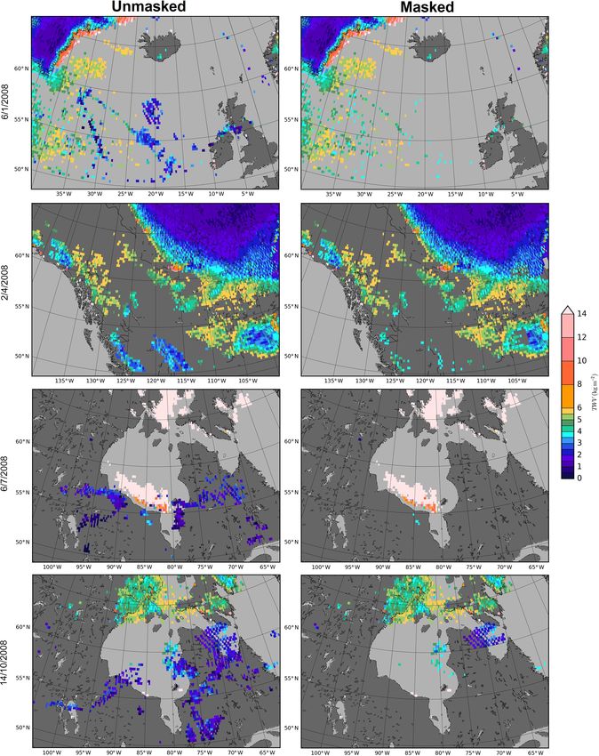
3698                 A. M. Triana-Gómez et al.: Improved water vapour retrieval from AMSU-B and MHS in the Arctic

crowave range, suitable space-borne instruments can in prin-       as groundwork for the planned merging with TWV retrieved
ciple ensure a complete global coverage of water vapour re-        over open ocean based on passive microwave imagers (prod-
trievals (Miao et al., 2001; Bobylev et al., 2010). In polar       uct described by Wentz and Meissner, 2006).
regions, however, satellite retrieval of water vapour faces a         In Sect. 2, we describe the algorithm in a more detailed
number of obstacles, such as cloud cover, which restricts          way. In Sect. 3 we evaluate the application of the algorithm
infrared measurements, or incomplete understanding of the          to MHS (Microwave Humidity Sounder) instead of AMSU-
high and highly variable sea ice emissivity, which challenges      B data, which is necessary for extending the dataset to cover
microwave measurements. Some studies, like the one by              recent years, performing a comparison with different in situ
Weaver et al. (2017), have been done for TWV in the Arc-           data sources in Sect. 3.2 and to ERA5 reanalysis in Sect. 3.3.
tic atmosphere, but none of them have been able to provide a       Following this, in Sect. 4 we evaluate the new ice cloud fil-
long-term Arctic-wide dataset.                                     tering developed for the algorithm in Sect. 4, and finally give
   An important step for Arctic water vapour retrieval comes       some conclusions in Sect. 5.
from the work of Miao et al. (2001). They used data from
the SSM/T2 (Special Sensor Microwave Humidity) humid-
ity sounder to develop an algorithm which was designed             2     Retrieval algorithm
to work in the Antarctic. The key concept of this method
is the use of several microwave channels with similar sur-         2.1    Data sources
face emissivity but different water vapour absorption. These
                                                                   The algorithm uses microwave radiometer satellite measure-
are the three channels near the 183.31 GHz water absorption
                                                                   ments from humidity sounders such as AMSU-B or MHS on
line (183.31 ± 1, ±3 and ±7 GHz), which, together with the
                                                                   board the NOAA (National Oceanic and Atmospheric Ad-
channel at the 150 GHz window frequency, allow retrieval of
                                                                   ministration) 15 to 19 satellites and EUMETSAT (European
TWV values up to about 7 kg m−2 . Above this value, two of
                                                                   Organisation for the Exploitation of Meteorological Satel-
the 183.31 GHz band channels become saturated and the sen-
                                                                   lites) Metop-A, Metop-B and Metop-C satellites. The char-
sor is not able to “see” through the whole atmospheric col-
                                                                   acteristics of each sensor can be found in Table 1, and the
umn anymore. In other words, when the TWV reaches a cer-
                                                                   launch dates of each satellite are given in Table 2. Through-
tain threshold, the brightness temperature at these Advanced
                                                                   out this paper, when we refer to AMSU-B TWV, the bright-
Microwave Sounding Unit-B (AMSU-B) channels does not
                                                                   ness temperature data used for the retrieval is always from the
change with increasing TWV (Miao, 1998; Melsheimer and
                                                                   sensor on NOAA-17, with the version from the Fundamental
Heygster, 2008). This limited range is enough for Antarc-
                                                                   Climate Data Record (Ferraro and Meng, 2016), which pro-
tica and suffices for the Arctic in winter conditions (in the
                                                                   vides an inter-satellite calibrated set of brightness tempera-
polar winter atmosphere, the water vapour column is typi-
                                                                   tures as described in Ferraro (2016). When we refer to MHS
cally around 3 kg m−2 , according to Serreze et al., 1995), as
                                                                   TWV, the brightness temperature data are from NOAA-18
well as for the central Arctic (above 70◦ N) most of the year.
                                                                   and are similarly sourced.
However, because of the upper limit, this method cannot en-
                                                                      Additionally, to distinguish between surface types, the
sure monitoring of the complete yearly cycle. The algorithm
                                                                   daily ice concentration provided by the ASI algorithm
developed by Melsheimer and Heygster (2008) extends the
                                                                   (ARTIST Sea Ice algorithm, Spreen et al., 2008) is used,
TWV retrieval range over sea ice by including the AMSU-
                                                                   with pixels with ice concentrations below 15% as open wa-
B (Advanced Microwave Sounding Unit-B) 89 GHz channel
                                                                   ter, while the ones with more than 80 % will be considered
into the retrieval. Using the triplet of the 183.31 ± 7, 150 and
                                                                   ice. The percentages between those will not be used.
89 GHz channels allows the retrieval to function up the satu-
ration limit of the 183.31 ± 7 GHz channel. This method has        2.2    Radiative transfer equation
been compared with other datasets. In Rinke et al. (2009) a
comparison with the HIRHAM model showed realistic pat-             The algorithm starts from the formulation of the radiative
terns and maximum root-mean-square differences (RMSDs)             transfer equation in the contracted form by Guissard and
for monthly data in summer of 1–2.5 kg m−2 . For the com-          Sobieski (1994), which describes the brightness temperature
parison with Ny-Ålesund radiosondes in Palm et al. (2010),         (TB ) measured by a space-borne radiometer as follows:
the correlation coefficient was 0.86 and the slope 0.8 ± 0.04.
And lastly, in Buehler et al. (2012) AMSU-B TWV are com-           TB (θ ) = mp Ts − (T0 − Tc )(1 − s )e−2τ sec θ ,           (1)
pared to GPS data from Kiruna, with a RMSD of 1 kg m−2
and a correlation coefficient of 0.86. However, the AMSU-          where θ is the zenith angle, Ts and T0 are the surface and
B algorithm is not without problem: while the frequency            air temperatures, respectively, Tc is the cosmic background
range allows it to bypass most clouds, the AMSU-B sensor           emission, s the surface emissivity, τ0 the total opacity of the
is still sensitive to convective clouds with high ice content.     atmosphere in the vertical direction, and mp a correction to
Here we provide an approach for filtering out problematic          take into account both a non-isothermal atmosphere and the
data caused by the effect of such ice clouds. This is intended     difference between the surface (skin) temperature, Ts , and

Atmos. Meas. Tech., 13, 3697–3715, 2020                                              https://doi.org/10.5194/amt-13-3697-2020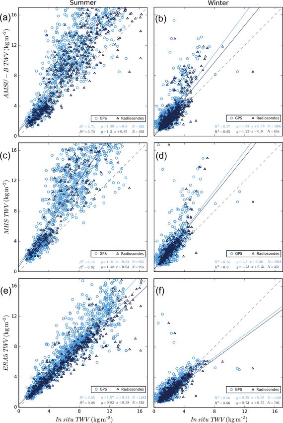
A. M. Triana-Gómez et al.: Improved water vapour retrieval from AMSU-B and MHS in the Arctic                                           3699

Table 1. Frequency and polarization details for each channel of AMSU-B and MHS sensors.

                                           AMSU-B                                        MHS
                             Channel      Frequency     Polarization   Channel      Frequency      Polarization
                                              (GHz)                                     (GHz)
                             16           89.9 ± 0.9    Vertical              1          89.9      Vertical
                             17          150.0 ± 0.9    Vertical              2         157.0      Vertical
                             18           183.31 ± 1    Vertical              3    183.31 ± 1      Horizontal
                             19           183.31 ± 3    Vertical              4    183.31 ± 3      Horizontal
                             20           183.31 ± 7    Vertical              5      190.311       Vertical

Table 2. Humidity sounders in orbit, with platforms, launch year       and j can be expressed as follows:
and approximate Equator crossing times (ECT).
                                                                       1Tij ≡ TBi − TBj = (T0 − Tc )(1 − s ),
            Platform    Sensor         Launch    ECT                          (e−2τi sec θ − e−2τj sec θ ) + bij ,                      (2)
                                         year
                                                                       where τi is the nadir opacity of the atmosphere at the fre-
            NOAA15      AMSU-B          1999    07:00
            NOAA16      AMSU-B          2000    21:00                  quency of channel i and bij is a bias related to the term mp
            NOAA17      AMSU-B          2002    07:00                  for the channels i and j :
            NOAA18      MHS             2005    20:00
                                                                       bij = Ts (mpi − mpj ).                                           (3)
            NOAA19      MHS             2009    20:00
            MetOp-A     MHS             2006    09:30                  As shown in Melsheimer and Heygster (2008), Appendix II,
            MetOp-B     MHS             2012    09:30
                                                                       the bias can here be approximated as follows:
            MetOp-C     MHS             2018    09:30
                                                                             Z∞h                                        i dT (z)
                                                                       bij ≈    e−2τi (z, ∞) sec θ − e−2τj (z, ∞) sec θ          dz,    (4)
                                                                                                                           dz
the temperature of the atmosphere at the ground, T0 (mp = 1                    0
would be the isothermal case and T0 = Ts ). The approach by            where T (z) is the atmospheric temperature profile. Then we
Melsheimer and Heygster (2008), summarized in the follow-              take the ratio of what we call compensated brightness tem-
ing, assumes the ground to be approximated as a specular re-           perature differences:
flector, which should be good enough for remote sensing in
the frequency range we are dealing with, according to Hewi-                   1T0ij    1Tij − bij    e−2τi sec θ − e−2τj sec θ
                                                                       ηc ≡          =              = −2τ sec θ                .        (5)
son and English (1999).                                                       1T0j k   1Tj k − bj k  e j         − e−2τk sec θ

2.3   Retrieval for equal emissivity assumption                        We can express the opacities τi as a sum of the atmospheric
                                                                       constituent contributions to them: water vapour (τiw ) and
                                                                                 oxygen
Note that the entire derivation of the final total water vapour        oxygen (τi       ). The latter is negligible for AMSU-B chan-
retrieval equation from the radiative transfer equation is de-         nels near the water vapour line, so if we take water vapour
scribed in detail in the initial paper for the Antarctic by            mass absorption coefficients ki and TWV W :
Miao et al. (2001) and the subsequent Arctic extension by                             oxygen
                                                                       τi = τiw + τi           ≈ ki W.                                  (6)
Melsheimer and Heygster (2008). We summarize it here be-
cause the basic mechanism is necessary to understand the               If we approximate the differences of exponentials by prod-
changes performed.                                                     ucts in Eq. (5) and take logarithms, we get the following
   We start from microwave radiometer satellite measure-               equation:
ments in three different channels i, j and k, as mentioned in
Sect. 2.1. We assume none of these three channels are satu-            ln(ηc ) = B0 + B1 W sec θ + B2 (W sec θ )2 .                     (7)
rated, i.e. the sensor is still sensitive to the whole atmospheric     The three constants B0 , B1 , and B2 depend on the mass
column and ground. Additionally, we take the ground emis-              absorption coefficients for the different channels. The term
sivity as equal in all three channels (as they see the same foot-      quadratic in W can be neglected (Selbach, 2003; Miao et al.,
print, and the emissivity does not vary between the channels),         2001), which leaves us with an equation linear in W that can
while the water vapour absorption (mass absorption coeffi-             then be solved to yield our retrieval equation:
cient k (m2 kg−1 )) is different, with ki < kj < kk . Following
this, the brightness temperature difference of two channels i          W sec θ = C0 + C1 ln(ηc ),                                       (8)

https://doi.org/10.5194/amt-13-3697-2020                                                    Atmos. Meas. Tech., 13, 3697–3715, 2020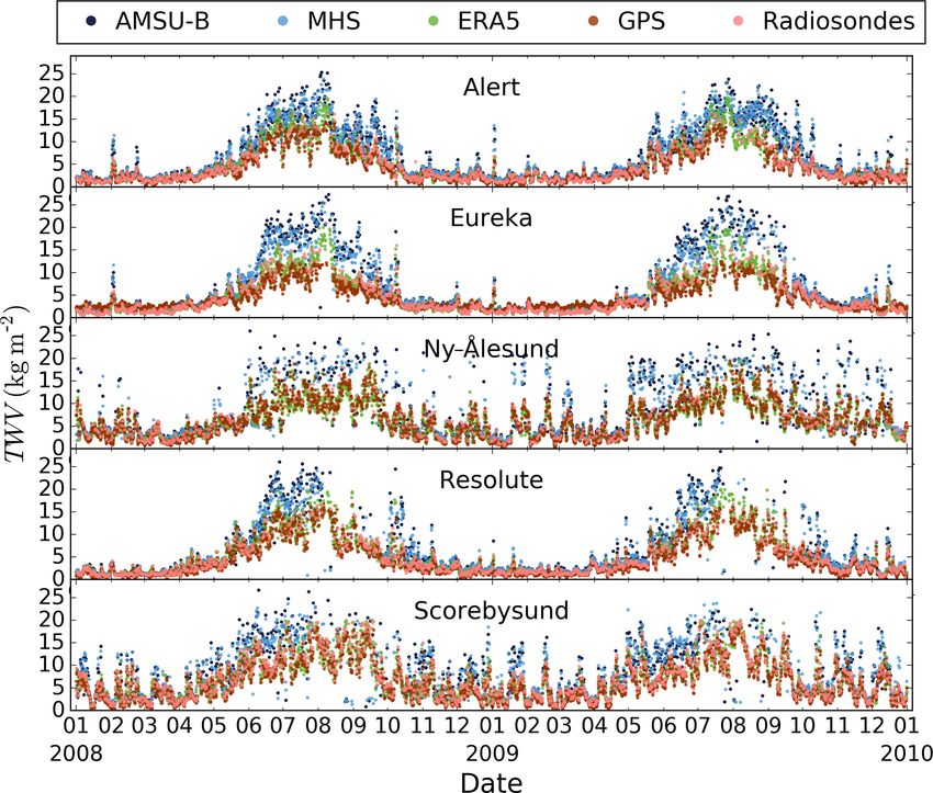
3700                   A. M. Triana-Gómez et al.: Improved water vapour retrieval from AMSU-B and MHS in the Arctic

                                                                        the others. Therefore, the retrieval equation needs to be re-
                                                                        derived with the changed premise: i 6 = j = k . This leaves
                                                                        us with a similar-looking retrieval equation:

                                                                        W sec θ = C0 + C1 ln(ηc0 ),                                 (9)

                                                                        where ηc0 is a modified ratio of compensated brightness tem-
                                                                        peratures:

                                                                                rj
                                                                        ηc0 ≡

                                                                                   ηc + C(τj , τk ) − C(τj , τk ),                 (10)
                                                                                ri

                                                                        and C(τj , τk ) is defined as follows:

                                                                                               e−2τj sec θ
                                                                        C(τj , τk ) =                           .                  (11)
                                                                                        e−2τj sec θ
                                                                                                  − e−2τk sec θ

                                                                        Since now there is a dependence on emissivities i , or, equiv-
                                                                        alently, on reflectivities ri = 1 − i , the surface emissivity
                                                                        at 89 GHz needs to be examined. Ideally, the ratio of cor-
                                                                        responding reflectivities would be taken for each footprint.
                                                                        However, that is not possible without knowing atmospheric
                                                                        conditions and surface temperature. As an approximation,
                                                                        the emissivity is parameterized, and fixed reflectivity ratios
                                                                        depending on surface types are obtained. This was done for
                                                                        sea ice in Melsheimer and Heygster (2008) and for open wa-
                                                                        ter surfaces in Scarlat et al. (2018). The upper limit of this
                                                                        extended retrieval is about 15 kg m−2 . Here, we will use this
                                                                        extended retrieval only over sea ice.

                                                                        2.5     The “sub-algorithms”: regime selection
Figure 1. Density plot and fit for MHS TWV vs. AMSU-B TWV
retrievals for all the coincident points in January (a) and July (b),   As described through Sects. 2.3 and 2.4, three different chan-
2008–2010. The dashed line is the one-to-one line, and the black        nel triplets are used for the retrieval, depending on the water
line corresponds to the linear fit of the data.                         vapour amount and the saturation of channels; hence, there
                                                                        are three “sub-algorithms” or retrieval regimes. Each sub-
                                                                        algorithm reaches its upper retrieval limit when the channel
              B0
where C0 = B   1
                 and C1 = B11 . They are determined empir-              that is most sensitive to water vapour becomes saturated. In
ically as calibration parameters from simulated brightness              the original algorithm formulation by Melsheimer and Heyg-
temperatures based on radiosonde profiles by a regression               ster (2008), the switch from one sub-algorithm to the next
analysis, described in more detail below (Sect. 2.6).                   (always starting with the most sensitive one) is done only
                                                                        when the following saturation condition is fulfilled:
2.4    Extension of the retrieval
                                                                        Tbj − Tbk > 0.                                             (12)
Normally, for TWV values above 7 kg m−2 , saturation oc-
curs at Channel 19 (183.3 ± 3 GHz). To extend the retrieval             This means that for each satellite footprint, only one of the
range above this threshold, another channel is required that            three sub-algorithms is finally used. As the sub-algorithms
is less sensitive to water vapour to take its place in the triplet.     have been calibrated independently, the switch from one to
This means that a new set of assumptions has to be made                 the next can cause a jump in the retrieved value. A method
about the surface emissivity influence. For AMSU-B, the                 avoiding this discontinuity in the retrieval values will be dis-
next channel “in line” is the one at 89 GHz (Channel 16).               cussed further in the follow-up paper. Additionally, as the
Thus, the three channels i, j and k are now the AMSU-                   switch between regimes is done in the brightness tempera-
B Channels 16, 17 and 20 (89, 150 and 183.31 ± 7 GHz).                  ture space, this does not correspond to a strict cut-off point
Because Channel 16 is so far from the other two, we can                 in water vapour. In Table 3 we summarize the characteristics
no longer assume that it has the same surface emissivity as             of each regime.

Atmos. Meas. Tech., 13, 3697–3715, 2020                                                     https://doi.org/10.5194/amt-13-3697-2020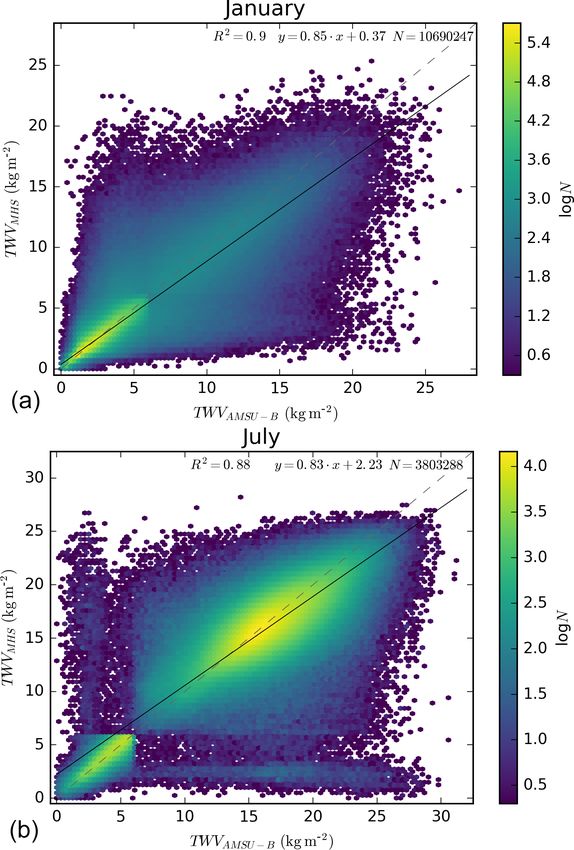
A. M. Triana-Gómez et al.: Improved water vapour retrieval from AMSU-B and MHS in the Arctic                                      3701

Table 3. Characteristics of the different sub-algorithms of the AMSU-B–MHS TWV retrieval. The channel combination is described with
AMSU-B frequencies, and the MHS retrieval uses the corresponding frequencies.

                    Sub-algorithm             Channel combination                Operating surface      Approximate
                                                                                                         limit TWV
                                                                                                           (kg m−2 )
                    Low               183.31 ± 7    183.31 ± 3    183.31 ± 1     Sea ice, ocean, land            1.5
                    Middle            183.31 ± 7    183.31 ± 3           150     Sea ice, ocean, land              7
                    Extended          183.31 ± 7           150            89     Sea ice                         15

Figure 2. Locations of the points chosen for the surface characterization study for TWV are shown in black. As background, the surface
classification used in the TWV algorithm, obtained from ASI algorithm ice concentration (Spreen et al., 2008) for a typical day in March
(6 March 2008) is given.

2.6   Bias and calibration parameters                                 the biases vanish; see Melsheimer and Heygster, 2008, Ap-
                                                                      pendix II). Having determined the focal point, the simulated
                                                                      brightness temperature differences and corresponding TWV
Since we ordered the channels by the water vapour sensitivity         values from the radiosonde profiles can be used to get the
(τi < τj < τk ), the difference of exponentials in 1T0ij and          calibration parameters C0 and C1 . Thus, together with the
1T0j k is negative. Therefore, the first term of the tempera-         two focal point coordinates Fj k and Fij , there is a total of
ture difference increases with increased emissivity from neg-         four calibration parameters in the retrieval equation which
ative values to 0 (reached when  = 1). ηc does not depend            are derived by this regression. The specific values for each
on , which cancels on the ratioing. In a plot with 1Tj k as          viewing angle and regime of AMSU-B sensor are found in
abscissa and 1Tij as ordinate, for constant W and varying ,          Melsheimer and Heygster (2008), Appendix III. For MHS,
this is a straight line with slope ηc (W ), running through the       all these calibration parameters were recalculated and are
bias points (bj k , bij ). Since the biases depend only weakly        shown in Appendix A.
on W and , all straight lines for different W run through
almost the same point F = (Fj k , Fij ), which is called focal        2.7      Filtering ice cloud artefacts
point by Miao et al. (2001) and Melsheimer and Heygster
(2008). The focal point F is found by simulating brightness           The effect of ice clouds at the AMSU-B frequencies as stud-
temperatures for a set of different , with different input at-       ied in Sreerekha (2005) is known and has been used for
mospheric profiles (including W ) from radiosonde data, and           detecting tropical deep convection (Hong et al., 2005) and
surface temperature taken as ground-level atmospheric tem-            for an automated method for finding polar mesocyclones
perature (which makes the small emissivity dependence of              (Melsheimer et al., 2016). The latter method uses the sen-

https://doi.org/10.5194/amt-13-3697-2020                                                  Atmos. Meas. Tech., 13, 3697–3715, 2020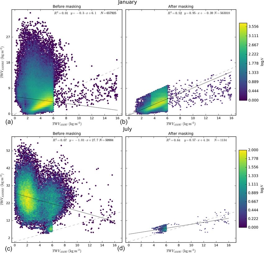
3702                A. M. Triana-Gómez et al.: Improved water vapour retrieval from AMSU-B and MHS in the Arctic

                                                                 almost entirely caused by strong convective clouds, which
                                                                 are typically organized in rather small-scale (tens of kilo-
                                                                 metres) cells or clusters thereof, or which take the shape of
                                                                 mesoscale structures such a polar lows with extents of at
                                                                 most a few hundred kilometres; even in large-scale, synop-
                                                                 tic low-pressure systems, convective clouds are organized in
                                                                 clusters and lines with the above-mentioned scales of tens
                                                                 to a few hundred kilometres. Therefore, image processing
                                                                 methods that rely on the size of ice cloud artefacts can be
                                                                 used. Our approach for eliminating the affected TWV is to
                                                                 find connected areas (with a minimum of two pixels) of low
                                                                 TWV (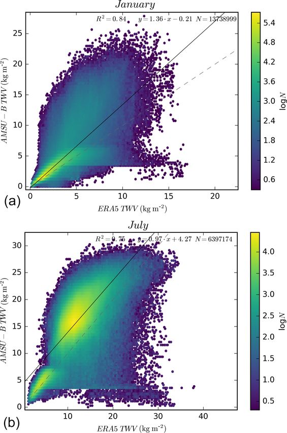
A. M. Triana-Gómez et al.: Improved water vapour retrieval from AMSU-B and MHS in the Arctic                                    3703

                                                                       satellite overpasses, and amount to only about 0.27 % of the
                                                                       data, so they are not significant in the overall picture.
                                                                          In Table 4, the fit statistics for all months are shown. The
                                                                       correlation ranges from 0.87 in June to 0.94 in September.
                                                                       The lowest slope (0.82) is found in December. On the other
                                                                       hand, the slope is closest to 1.0 in May (0.91). The intercept
                                                                       increases for the summer months (June, July, August) but is
                                                                       relatively small for the other months. The RMSD has a sim-
                                                                       ilar behaviour: we find higher values for the central months
                                                                       of the year, with a maximum of 2.25 kg m−2 in August, coin-
                                                                       ciding with the increased number of outliers. The minimum
                                                                       is 0.73 kg m−2 in March. The bias is generally small (min-
                                                                       imum of 0.04 kg m−2 in March, maximum of 0.49 kg m−2
                                                                       in September), and positive except for May and June. In
                                                                       general, all parameters show the lowest agreement in the
                                                                       summer months when the atmospheric variability is highest.
                                                                       However, we presume the strongest contribution to the lower
                                                                       agreement in summer is due to the higher uncertainty and
Figure 5. Scatter plot and fit for MHS TWV vs. radiosonde TWV          variability in the surface emission due to melt process and
retrievals for all coincident points during the N-ICE campaign. The    occurrence of melt ponds.
colour scale shows the month where the data point comes from. The         To check any possible influence from the surface type in
dashed line shows the one-to-one lines, and the solid line shows the   the consistency of our retrievals, we have studied the TWV
linear regression.                                                     time series during 2008–2009 for MHS and AMSU-B over
                                                                       different surfaces: ice, land and open water. The location cho-
                                                                       sen for each study point is shown in Fig. 2, with the surface
                                                                       classification used in the TWV retrieval for a day in early
                                                                       March 2008 (maximum ice extent) as background. We show
                                                                       the monthly and yearly means of this time series for the four
                                                                       different locations in Fig. 3. Note the lack of data for sum-
                                                                       mer months over open water and ocean because of the limita-
                                                                       tions of the algorithm. All four time series show good agree-
                                                                       ment, which confirms the consistency between our retrievals.
                                                                       The bias and RMSD are small for all four surface types (ice:
                                                                       0.1 ± 0.4 kg m−2 ; open water: 0.03 ± 0.15 kg m−2 ; marginal
                                                                       ice zone: 0.2 ± 0.7 kg m−2 ; land: 0.12 ± 0.19 kg m−2 ) but
                                                                       slightly higher in two cases with ice surfaces, which agrees
                                                                       with the higher error of our method for higher water vapour
                                                                       values (extended regime).

                                                                       3.2   Comparison with in situ data sources

                                                                       While TWV retrieved from AMSU-B has been validated
Figure 6. Location of the radiosonde and GPS stations.                 with different data sources (Rinke et al., 2009; Palm et al.,
                                                                       2010; Buehler et al., 2012), the same cannot be said about the
                                                                       retrieval with MHS data. Therefore, we perform a compari-
analysis, we considered all the coincident points in the daily         son with TWV derived from radiosondes taken during the
gridded data with a 0.25◦ grid. Figure 1 shows two den-                N-ICE2015 campaign from January to June 2015 onboard re-
sity plots for the overlap months of January (top) and July            search vessel Lance north of Svalbard (Hudson et al., 2017;
(bottom) of 2008–2009. The results of a least-squares re-              Cohen et al., 2017). We select the MHS data as the mean of
gression are shown in the figure as well. Both datasets show           all the values in a 50 km radius around the location of each
good agreement, with most of the points along the one-to-one           radiosonde. The resulting time series is shown in Fig. 4. The
line. However, we can observe some outliers with high MHS              first thing to note is that the MHS series ends at the start of
TWV and low, almost constant, AMSU-B TWV, and vice                     June because, afterward, the surface in the area is consid-
versa, especially striking during the month of July. These             ered mixed according to the criteria described in Sect. 2.1.
points are mostly associated with time differences of the              However, both datasets show good visual agreement, except

https://doi.org/10.5194/amt-13-3697-2020                                                Atmos. Meas. Tech., 13, 3697–3715, 2020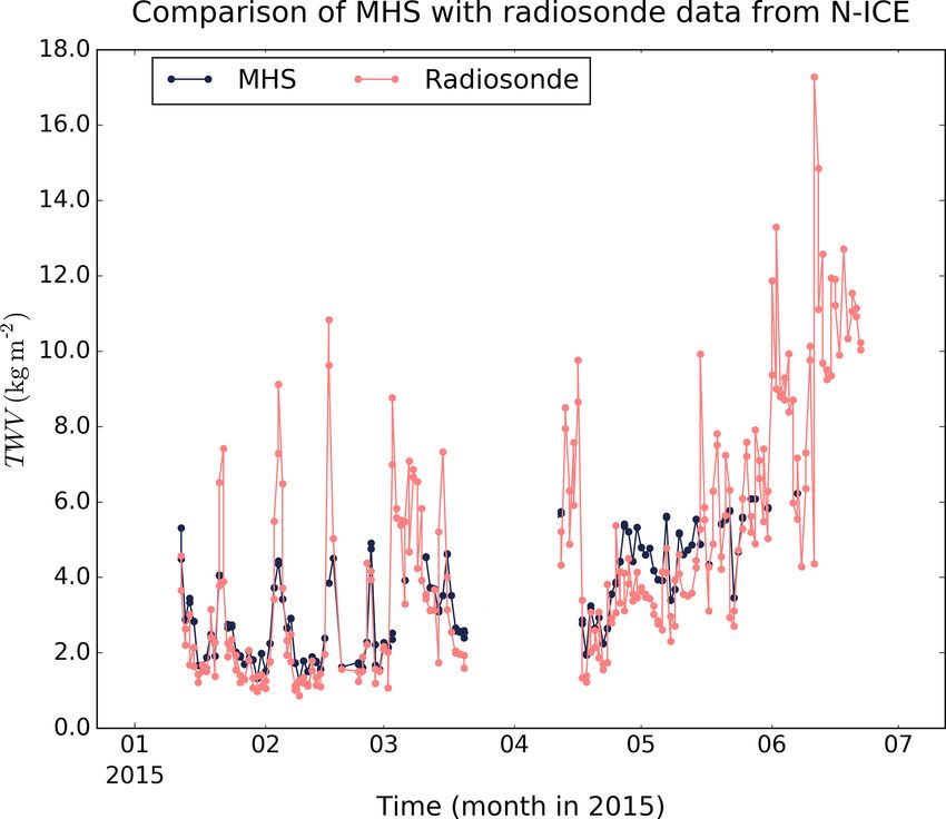
3704                 A. M. Triana-Gómez et al.: Improved water vapour retrieval from AMSU-B and MHS in the Arctic

Figure 7. Time series of AMSU-B (dark blue), MHS (light blue), ERA5 (green), GPS (purple) and radiosonde (salmon) TWV retrievals
during 2008 and 2009.

Table 4. Parameters for linear regression for monthly MHS and AMSU-B intercomparison.

                            Month         R2    Slope     Intercept     RMSD           Bias   Number of
                                                         (kg m−2 )    (kg m−2 )   (kg m−2 )      points
                            January      0.90    0.85         0.37         0.97        0.06   10 691 385
                            February     0.89    0.84         0.38         0.87        0.05    9 858 305
                            March        0.90    0.87         0.31         0.73        0.04   10 389 349
                            April        0.90    0.88         0.40         1.02        0.06    8 592 621
                            May          0.91    0.91         0.61         1.59       -0.02    6 087 842
                            June         0.87    0.84         2.33         2.25       -0.38    4 741 678
                            July         0.88    0.83         2.23         2.18        0.38    3 803 287
                            August       0.92    0.88         1.43         2.07        0.35    3 272 951
                            September    0.94    0.89         0.83         1.77        0.49    3 630 497
                            October      0.93    0.86         0.67         1.55        0.19    6 000 153
                            November     0.90    0.85         0.53         1.20        0.06    8 610 697
                            December     0.88    0.82         0.50         1.24        0.12    7 723 324

that MHS is not able to capture some of the quasi periodic               Additionally, we used global positioning system (GPS)
peaks in TWV from N-ICE2015 dataset (seen roughly ev-                 and radiosounding (RS) TWV observations during the com-
ery 2 weeks in February and March). We have eliminated                mon 2008–2009 period between the AMSU-B and MHS sen-
these nine outliers associated with the quasi periodic peaks          sors to evaluate the satellite TWV retrieval. GPS and ra-
in TWV from the following analysis. The scatter plot of all           diosonde TWV have been measured at the five coastal Arctic
overlapping points of both datasets, with the colour scale rep-       stations Alert, Eureka, Ny-Ålesund, Resolute and Scoreby-
resenting the month of the campaign (shown in Fig. 5) con-            sund, as shown in Fig. 6. These datasets are part of a homog-
firms the good agreement.                                             enized time series. From the GPS data, 1 h average values
                                                                      of local integrated TWV have been computed each 6 h. The

Atmos. Meas. Tech., 13, 3697–3715, 2020                                               https://doi.org/10.5194/amt-13-3697-2020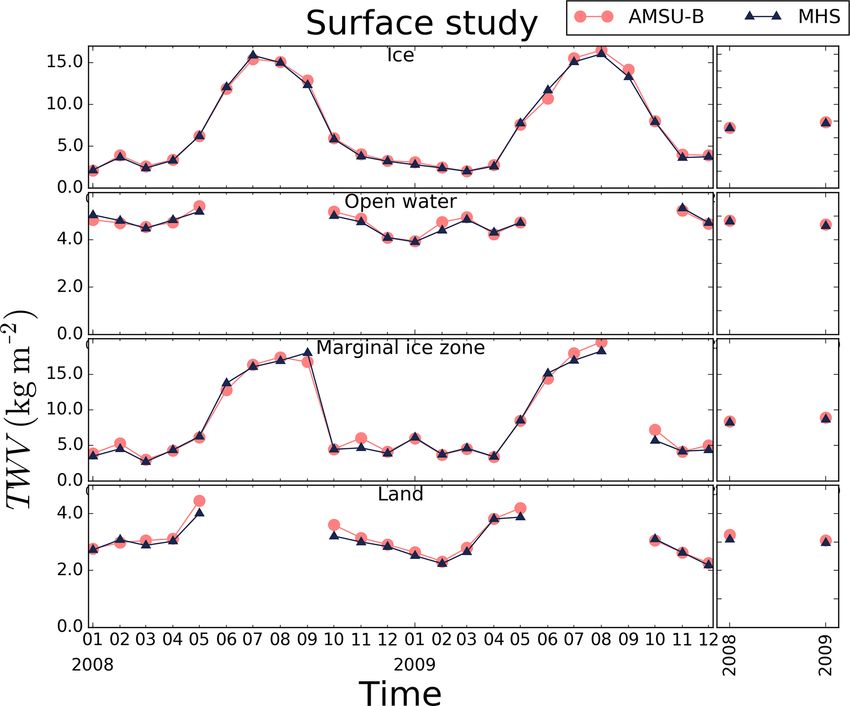
A. M. Triana-Gómez et al.: Improved water vapour retrieval from AMSU-B and MHS in the Arctic                                             3705

Figure 8. Scatter plots and fits for AMSU-B (a, b), MHS (c, d) and ERA5 (e, f) TWV retrievals vs. GPS (light blue) and radiosonde (dark
blue) TWV retrievals for all coincident points during summer (a, c, e) and winter (b, d, f) 2008 and 2009 at the Alert station. The solid lines
in light and dark blue show the linear regressions for GPS and radiosondes in each case, while the dashed lines are the identity line.

https://doi.org/10.5194/amt-13-3697-2020                                                     Atmos. Meas. Tech., 13, 3697–3715, 2020
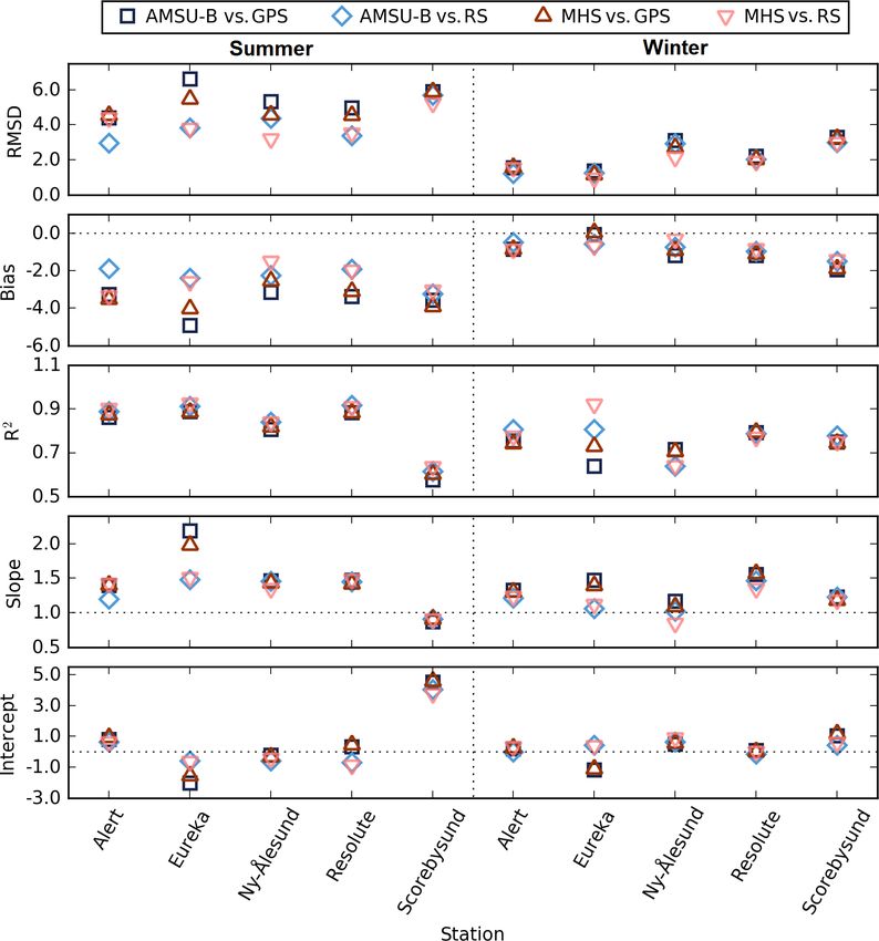
3706                  A. M. Triana-Gómez et al.: Improved water vapour retrieval from AMSU-B and MHS in the Arctic

Figure 9. Values of fit parameters for summer (left column) and winter (right column): RMSD, bias, correlation coefficient R2 , slope, and
intercept of regression line for MHS and AMSU-B TWV retrievals vs. radiosonde and GPS TWV retrievals. RMSD, bias and intercept are
given in kg m−2 , and slope and R2 are absolute numbers.

radiosoundings have been performed once or twice per day               March) in the following analysis. There seems to be a slight
at the selected sites (00:00 and 12:00 UTC). Further details           wet bias in summer for both satellite-derived TWV with re-
about processing can be found in Negusini et al. (2016). As            spect to the other datasets.
for the AMSU-B and MHS TWV values, we selected points                     Scatter plots comparing each dataset (both satellite and re-
fulfilling the data conditions of ±1 h from the integrated             analysis) with both radiosondes and GPS have been prepared
GPS measurements (00:00, 06:00, 12:00 and 18:00 UTC)                   for each season and station. As an example, Fig. 8 shows the
and found in a 50 km radius around the GPS and RS stations.            results for Alert. The correlation coefficients vary between
Additionally, TWV data from ERA5 reanalysis (Copernicus                0.55 to 0.88, and the correlations in winter seems to be gener-
Climate Change Service, C3S, 2017) were obtained using                 ally lower. We presume this is just a numerical effect because
the same conditions. The resulting AMSU-B, MHS, ERA5,                  of the narrower data distribution. The RMSD, in contrast, is
GPS and radiosonde time series in Fig. 7 present generally             higher in summer (as seen in Fig. 9). The only difference
consistent patterns and reasonable seasonal evolution, with            between both satellite-based retrievals seems to be a smaller
drier winters and wetter summers. Overall, the datasets have           number of coincident points between the MHS TWV and the
worse agreement during the summer months, mainly due to                radiosondes TWV (approximately half of the data points).
“spikier” data, i.e. more extreme water vapour values. Due to             Figure 9 shows all fit parameters for the five stations, with
this pronounced seasonal cycle, we separate the results be-            separated results between summer and winter. There seems
tween summer (April to September) and winter (October to               to be only little difference between the results from the two

Atmos. Meas. Tech., 13, 3697–3715, 2020                                                  https://doi.org/10.5194/amt-13-3697-2020
A. M. Triana-Gómez et al.: Improved water vapour retrieval from AMSU-B and MHS in the Arctic                                       3707

                                                                         age for all stations) but underestimate data to a higher de-
                                                                         gree in winter (on average 0.85 for GPS and 0.76 for ra-
                                                                         diosondes). This seasonal variation is similar for the corre-
                                                                         lation coefficient, higher in summer (averaging 0.9 and 0.92)
                                                                         and lower in winter, 0.85 and 0.75 for GPS and radioson-
                                                                         des, respectively. These values are very similar to the aver-
                                                                         ages for the satellite data vs. the in situ data. The RMSD and
                                                                         bias are generally small but smaller in winter. The average
                                                                         RMSD is 1.89 kg m−2 in summer and 1.10 kg m−2 in winter
                                                                         for GPS and 1.58 kg m−2 in summer and 1.05 kg m−2 in win-
                                                                         ter for radiosondes. The average bias is generally negative for
                                                                         GPS, averaging −0.5 kg m−2 in summer and −0.02 kg m−2
                                                                         in winter, while it is always positive for radiosondes, averag-
                                                                         ing 0.34 kg m−2 in summer and 0.17 kg m−2 in winter.

                                                                         3.3   Comparison with ERA5 reanalysis

                                                                         The reanalysis product ERA5 combines a variety of obser-
                                                                         vations and a numerical model using an optimization pro-
                                                                         cedure. Due to ERA5 assimilation of some of the observa-
                                                                         tions used as verification here, namely radiosondes, it is not
                                                                         a completely independent estimate of TWV. ERA5 also as-
                                                                         similates some 183GHz data over sea ice and snow-covered
                                                                         surfaces (as suggested in Bormann et al., 2017), including
                                                                         the MHS sounding channels. While it is unclear to the au-
                                                                         thors which sensors would have been available and assim-
                                                                         ilated within ERA5 for the time period 2008–2010 of this
                                                                         study, we cannot presume that ERA5 TWV is entirely inde-
                                                                         pendent of microwave humidity sounder radiances.
                                                                            For this study, we have compiled all the overlapping daily
                                                                         means of TWV from AMSU-B and ERA5 (Copernicus Cli-
                                                                         mate Change Service, C3S, 2017) for the complete months of
Figure 10. Density plot and fit for AMSU-B TWV vs. ERA5 TWV              January (top) and July (bottom) from 2008 to 2009, shown in
retrievals for all the coincident points in January (a) and July (b)
                                                                         Fig. 10. The results of a least-squares regression are shown
from 2008 to 2009, with a fit (solid black line) for the data clusters
over the one-to-one line (dashed grey).
                                                                         in Fig. 10 as well. Both datasets show good agreement, with
                                                                         most of the points along or parallel to the one-to-one line.
                                                                         Low AMSU-B TWV values compared to high ERA5 TWV
satellite-based retrievals, which corroborates our confidence            values can be observed in both months but are more promi-
in the MHS-based retrieval. Over the three quality-indicating            nent in summer. These are remnants of ice cloud artefacts
parameters, RMSD, bias and correlation coefficient, there is             that were not entirely filtered out.
even a slight but consistent advantage for the MHS-based                    Table 5 shows the fit statistics for all months. The correla-
retrieval. The bias values are almost all negative, and the              tion ranges from 0.71 in June to 0.88 in December. The worst
RMSD is along usual values for TWV studies at high lati-                 slope (1.6) is found in September. On the other hand, the
tudes (as seen in Palm et al., 2010, for Ny-Ålesund and in               slope is closest to 1.0 in August (0.97). However, the RMSD
Buehler et al., 2012, for Kiruna), which reassures us of the             has higher values for summer months of the year, with a max-
quality of satellite-based TWV retrievals. The higher RMSD               imum of 5.9 kg m−2 in August, coinciding with the increased
values in the Arctic summer in Fig. 9 can also be seen at                number of outliers. The minimum is 1.00 kg m−2 in March.
high TWV values over 7 kg m−2 during summer for all meth-                The bias is generally negative and shows similar behaviour to
ods in Fig. 8a and c. One explanation for the smaller bias and           the RMSD. In general, all parameters show the lowest agree-
RMSD during winter can be that also the absolute values dur-             ment in the summer months when the atmospheric variability
ing winter are small. The reason for a low correlation is likely         is highest.
that the temporal coherence is less pronounced.
   When fits like in Fig. 8 are performed for all stations for
ERA5 vs. GPS and radiosondes, the slopes are closer to one
in summer (0.99 for GPS and 0.87 for radiosondes on aver-

https://doi.org/10.5194/amt-13-3697-2020                                                   Atmos. Meas. Tech., 13, 3697–3715, 2020
3708 A. M. Triana-Gómez et al.: Improved water vapour retrieval from AMSU-B and MHS in the Arctic Figure 11. AMSU-B (top row), MHS (second row), AMSR-E (third row) and ERA5 (bottom row) TWV retrievals for winter (6 January 2008; left column) and summer (6 July 2008; right column). Atmos. Meas. Tech., 13, 3697–3715, 2020 https://doi.org/10.5194/amt-13-3697-2020
A. M. Triana-Gómez et al.: Improved water vapour retrieval from AMSU-B and MHS in the Arctic 3709
ferent data product based on AMSR-E observations (Wentz
and Meissner, 2006) over open ocean (third row) and ERA5
reanalysis daily mean (bottom row) in winter (left column)
and summer (right column). The days chosen to represent
each season (6 January and 6 July 2008, respectively) show
what a typical retrieval looks like for the respective season.
The first thing to notice is the difference in spatial cover-
age of AMSU-B TWV between winter and summer. In sum-
mer, AMSU-B–MHS retrieval is restricted to the drier re-
gions, mostly over sea ice and Greenland (the upper limit
of the retrieval is usually about 15 kg m−2 for sea ice sur-
faces). In winter, the retrieval is possible over most of the
land, open water areas and sea ice. Meanwhile, there is no
significant coverage variation shown between seasons for the
AMSR-E retrieval: most open water areas are covered. As a
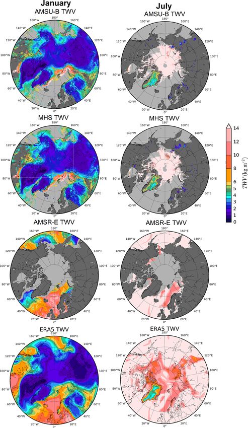
consequence, the area covered by both methods is smaller in
summer, as we can note in the map illustrating the regional
coverage (for the same days) of both algorithms in Fig. 12
(orange area shows joint coverage). Still, TWV is retrieved
in most of the Arctic in both seasons. Another consequence
is that in summer the overlap area is small. In this particular
example of Fig. 12, there is no overlap between both datasets.
As for the ERA5 dataset, the agreement with both AMSU-B
and AMSR-E is qualitatively good, showing similar patterns,
particularly in winter.
To visualize the areas affected by the ice cloud artefact,
Fig. 13 shows different areas of interest before (left) and af-
ter (right) filtering, for different days spaced evenly through-
out 2008 (approximately every 3 months: 6 January, 2 April,
6 July and 14 October). These areas have been chosen as
representative cases for the season. Most features (small re-
gions of low TWV surrounded by high TWV) are removed,
but there are still some small areas of low values of TWV
(such as the retrieved regions in the land around 62◦ N, 70◦ W
Fig. 13 (October, bottom right)). Note that these incorrectly
retrieved areas are surrounded by grey values which repre-
sent water vapour too high to be retrieved with the AMSU-B
method (about >7 kg m−2 over ocean or land surfaces). We
confirmed by comparison to the ERA5 atmospheric reanal-
ysis that the remaining high TWV values are within the ex-
pected range. Also the high, >14 kg m−2 , TWV values on
6 July 2008 in the Hudson Bay area are in agreement with
ERA5.
Figure 12. Coverage and overlap area of the merged AMSU-B and To show the overall effectiveness of the ice cloud filtering,
AMSR-E retrieval for (a) winter (6 January 2008) and (b) summer we have compiled all the overlapping retrieved TWV from
(6 July, 2008). Note that there is no overlap between retrievals (or- AMSU-B and AMSR-E for the complete months of January
ange) for the summer case presented. (Fig. 14a, b) and July (Fig. 14c, d) from 2006 to 2008. Be-
fore filtering for ice cloud artefacts (Fig. 14a, c), there is a
big cluster of data with high AMSR-E values for relatively
4 Evaluation of changes and improvements in the low AMSU-B values. Those correspond to the values af-
retrieval: filtering ice cloud artefacts fected by convective clouds with high ice content. Note that
the overlap area between AMSR-E and AMSU-B is small
Figure 11 shows daily averaged TWV maps with the ice (Fig. 12) and therefore cloud artefacts make up a large frac-
cloud filtering (Sect. 2.7) already applied for the AMSU-B– tion of the overlap data points, particularly in summer. Af-
MHS algorithm (top and second row), as well as from a dif- ter filtering (Fig. 14b, d) the AMSU-B retrieval, they are
https://doi.org/10.5194/amt-13-3697-2020 Atmos. Meas. Tech., 13, 3697–3715, 20203710 A. M. Triana-Gómez et al.: Improved water vapour retrieval from AMSU-B and MHS in the Arctic Figure 13. Unmasked (left column) and masked (right column) AMSU-B TWV retrieval for different showcased areas of 4 d in 2008: 6 January (top row), 2 April (second row), 6 July (third row) and 14 October (bottom row). Please note the different location in each case. Atmos. Meas. Tech., 13, 3697–3715, 2020 https://doi.org/10.5194/amt-13-3697-2020
A. M. Triana-Gómez et al.: Improved water vapour retrieval from AMSU-B and MHS in the Arctic                                                 3711

Figure 14. Density plot and fit for AMSR-E TWV vs. AMSU-B TWV retrievals for all the coincident points in January (a, b) and July (c,
d) from 2006 to 2008, both before (a, c) and after (b, d) filtering AMSU-B retrieval for ice cloud artefacts, with a fit (solid black line) for the
data clusters over the one-to-one line (dashed grey).

gone. Additionally, the fit performed improves significantly,               age 55.5 %. In winter, the values from the overlap area aver-
with the correlation reaching 0.6 in summer and the slope                   age 11.8 %.
getting much closer to one in winter (0.95, as compared to
0.3). Note also the jump in density of the retrieved TWV val-
ues caused by switching between sub-algorithms mentioned
above (Sect. 2.5), most notably near 6 kg m−2 (Fig. 14). Be-                5   Conclusions
tween 7.6 % (January) and 11 % (March) of the data are
masked by the ice cloud filter for winter months, while the                 We provide an updated version of the TWV retrieval al-
percentage is much smaller in the summer months, ranging                    gorithm that originally uses as input microwave humidity
between 0.18 % of the data in August to 3.7 % in June. In                   sounder data from AMSU-B. The updated algorithm can now
summer, up to 94 % of those values (July) come from the                     also use data from MHS, the successor instrument of AMSU-
overlap area between AMSU-B and AMSRE, with the aver-                       B, and contains a filter for artefacts caused by convective
                                                                            clouds with high cloud ice content. The improved retrieval

https://doi.org/10.5194/amt-13-3697-2020                                                        Atmos. Meas. Tech., 13, 3697–3715, 2020
3712 A. M. Triana-Gómez et al.: Improved water vapour retrieval from AMSU-B and MHS in the Arctic
Table 5. Parameters for linear regression for monthly AMSU-B and ERA5 intercomparison.
Month R2 Slope Intercept RMSD Bias Number of
(kg m−2 ) (kg m−2 ) (kg m−2 ) points
January 0.84 1.36 −0.22 1.43 −0.58 13 738 999
February 0.85 1.33 −0.2 1.25 −0.52 12 626 117
March 0.85 1.17 0.06 1.00 −0.44 14 004 549
April 0.84 1.16 0.12 1.38 −0.61 11 891 174
May 0.78 1.25 −0.19 2.72 −1.21 8 511 599
June 0.71 1.11 1.69 4.32 −2.72 7 212 136
July 0.75 0.97 4.28 4.89 −3.87 6 397 174
August 0.73 0.97 5.1 5.91 −4.79 5 376 590
September 0.81 1.54 0.95 5.83 −4.77 5 692 249
October 0.74 1.67 −0.24 3.54 −2.11 9 281 562
November 0.77 1.5 −0.41 2.1 −1.05 11 880 942
December 0.88 0.82 0.50 1.24 0.12 10 822 902
performs better when compared to another satellite product The filter for ice cloud artefacts performs well, as shown
and to in situ data. by comparison with data from the AMSR-E-based algo-
The coefficients in the retrieval algorithm were adapted rithm that works over open water. A remaining issue is the
for MHS (Appendix A). We have investigated the impact jumps of retrieved TWV values between the different re-
of differences between AMSU-B and MHS on the retrieved trieval regimes. This can, however, in principle be mitigated
TWV and have found the differences to be negligible. This by comparing root-mean-square differences and bias for ad-
means that a consistent continuous dataset for the years jacent TWV regimes and choosing an optimal regime, i.e.
1999 until 2020 can be generated from combining AMSU- channel combination, for the range of the water vapour col-
B and MHS data. Additionally, the MHS-based TWV data umn. Where regimes overlap, weighted averages can smooth
have been compared with radiosonde data from the N- the transition.
ICE2015 campaign, and the results show good performance The algorithm described here has an upper TWV limit that
for MHS TWV. Both satellite-derived TWV have been com- restricts retrieval in summer to the central Arctic and Green-
pared against GPS and radiosonde data for five Arctic coastal land. However, when combining the TWV data retrieved by
stations during 2008 and 2009, and the results are satisfac- the algorithm described here with TWV retrieved over open
tory, with averaged correlations for all stations and methods ocean from AMSR-E and AMSR2, a product of remote sens-
0.82 in summer and 0.75 in winter and RMSD along usual ing systems (RSSs) (Wentz and Meissner, 2006), a nearly
values for TWV studies at high latitudes. The satellite-based complete year-round coverage of the whole Arctic is possi-
TWV retrieval also compares well with the ERA5 reanalysis. ble, starting in 2000, which is the overall goal of future work.
Some artefacts of unfiltered ice clouds remain, but overall the
correlation with 0.79 and RMSD of 3.01 kg m−2 shows good
correspondence.
Atmos. Meas. Tech., 13, 3697–3715, 2020 https://doi.org/10.5194/amt-13-3697-2020A. M. Triana-Gómez et al.: Improved water vapour retrieval from AMSU-B and MHS in the Arctic 3713
Appendix A
The following tables list the calibration parameters C0 , C1 ,
Fj k and Fij for the TWV retrieval algorithm for the Arctic
and (for the sake of completeness) the Antarctic, for 15 view- Table A2. Calibration parameters for the Arctic mid-TWV algo-
ing angles that span the range of the viewing angles of MHS, rithm.
calculated in the same way as the parameters for AMSU-
θ C0 C1 M
F5, M
F2,
B-based retrieval by Melsheimer and Heygster (2008). The 4 5
retrieval equation is taken from Eqs. (5) and (8) as follows: [kg m−2 ] [kg m−2 ] [K] [K]
1Tij − Fij
1.667◦ 1.63 2.64 6.56 5.74
W sec θ = C0 + C1 ln , (A1) 5.000◦ 1.63 2.64 6.55 5.75
1Tj k − Fj k 8.333◦ 1.62 2.64 6.54 5.75
11.667◦ 1.61 2.63 6.52 5.75
where 1Tij = Tb, i − Tb, j and the MHS channels i, j and k
15.000◦ 1.60 2.62 6.50 5.77
are 18.333◦ 1.59 2.61 6.46 5.77
21.667◦ 1.57 2.59 6.43 5.79
– 5 (190.31 GHz), 4 (183.31 ± 3 GHz), and 3 (183.31 ±
25.000◦ 1.55 2.57 6.38 5.82
1 GHz) for the low-TWV algorithm;
28.333◦ 1.53 2.54 6.34 5.86
– 2 (157 GHz), 5 (190.31 GHz), and 4 (183.31 ± 3 GHz) 31.667◦ 1.50 2.50 6.25 5.86
35.000◦ 1.46 2.46 6.18 5.90
for the mid-TWV algorithm;
38.333◦ 1.42 2.40 6.09 5.95
and from Eqs. (10) and (9) as follows: 41.667◦ 1.37 2.33 5.99 6.01
45.000◦ 1.30 2.24 5.83 6.03
48.333◦ 1.22 2.11 5.65 6.08
rj 1Tij − Fij
W sec θ = C0 + C1 ln + 1.1 − 1.1 , (A2)
ri 1Tj k − Fj k
where i, j and k are 1 (89.9 GHz), 2 (157 GHz) and 5
(190.31 GHz) for the extended algorithm.
The calibration parameters for the Arctic (Tables A1–A3)
were derived using radiosonde data from those World Meteo-
rological Organization (WMO) stations in the Arctic that are
located on the coast or on islands (29 stations), from the years
1996 to 2002, which amounts to about 27 000 radiosonde
profiles. Table A3. Calibration parameters for the Arctic extended algorithm.
Table A1. Calibration parameters for the Arctic low-TWV algo- θ C0 C1 E
F2, E
F1,
5 2
rithm. [kg m−2 ] [kg m−2 ] [K] [K]
θ C0 C1 L
F4, L
F5, 1.667◦ 14.4 7.45 6.52 0.74
3 4
[kg m−2 ] [kg m−2 ] [K] [K] 5.000◦ 14.4 7.47 6.55 0.74
8.333◦ 14.4 7.50 6.61 0.75
1.667◦ 0.619 1.05 4.86 4.43 11.667◦ 14.4 7.56 6.71 0.77
5.000◦ 0.619 1.05 4.87 4.45
15.000◦ 14.4 7.63 6.84 0.80
8.333◦ 0.618 1.05 4.90 4.50
11.667◦ 0.617 1.05 4.94 4.58 18.333◦ 14.4 7.73 7.00 0.83
15.000◦ 0.615 1.05 4.99 4.68 21.667◦ 14.5 7.83 7.20 0.87
18.333◦ 0.613 1.05 5.06 4.81 25.000◦ 14.5 7.97 7.44 0.93
21.667◦ 0.609 1.05 5.14 4.97 28.333◦ 14.5 8.11 7.72 1.00
25.000◦ 0.606 1.04 5.23 5.16 31.667◦ 14.5 8.26 8.04 1.08
28.333◦ 0.601 1.04 5.32 5.36 35.000◦ 14.5 8.43 8.41 1.19
31.667◦ 0.598 1.02 5.31 5.41 38.333◦ 14.4 8.60 8.83 1.33
35.000◦ 0.597 1.00 5.25 5.36 41.667◦ 14.2 8.76 9.30 1.50
38.333◦ 0.602 0.96 5.01 4.96
45.000◦ 13.9 8.90 9.83 1.74
41.667◦ 0.603 0.92 4.76 4.50
45.000◦ 0.607 0.87 4.43 3.85 48.333◦ 13.4 8.99 10.4 2.04
48.333◦ 0.607 0.80 4.12 3.27
https://doi.org/10.5194/amt-13-3697-2020 Atmos. Meas. Tech., 13, 3697–3715, 20203714 A. M. Triana-Gómez et al.: Improved water vapour retrieval from AMSU-B and MHS in the Arctic
Data availability. The datasets generated and analyzed in this References
study are available from the corresponding author on reasonable
request. The AMSU-B and MHS datasets generated will be avail-
able in the near future at https://seaice.uni-bremen.de/ (Triana et al., Bobylev, L. P., Zabolotskikh, E. V., Mitnik, L. M., and Mit-
2020). nik, M. L.: Atmospheric Water vapour and Cloud Liquid Wa-
ter Retrieval over the Arctic Ocean Using Satellite Passive
Microwave Sensing, IEEE T. Geosci. Remote, 48, 283–294,
Author contributions. AMTG wrote the initial manuscript draft, https://doi.org/10.1109/TGRS.2009.2028018, 2010.
made the figures, and processed the AMSU-B and MHS TWV. Buehler, S. A., Östman, S., Melsheimer, C., Holl, G., Eliasson, S.,
CM calculated the calibration parameters shown in Appendix A John, V. O., Blumenstock, T., Hase, F., Elgered, G., Raffalski,
and wrote the original algorithm code. GS, CM and GH provided U., Nasuno, T., Satoh, M., Milz, M., and Mendrok, J.: A multi-
scientific feedback and discussion. MN and BHP provided the instrument comparison of integrated water vapour measurements
GPS and radiosonde data, respectively. All co-authors reviewed the at a high latitude site, Atmos. Chem. Phys., 12, 10925–10943,
manuscript. https://doi.org/10.5194/acp-12-10925-2012, 2012.
Chahine, M.: The hydrological cycle and its influence on climate,
Nature, 359, 373–380, 1992.
Cohen, L., Hudson, S. R., Walden, V. P., Graham, R. M.,
Competing interests. The authors declare that they have no conflict
and Granskog, M. A.: Meteorological conditions in a
of interest.
thinner Arctic sea ice regime from winter to summer
during the Norwegian Young Sea Ice expedition (N-
ICE2015), J. Geophys. Res.-Atmos., 122, 7235–7259,
Acknowledgements. AMSR TWV data are produced by Remote https://doi.org/10.1002/2016JD026034, 2016JD026034, 2017.
Sensing Systems and were sponsored by the NASA AMSR-E Sci- Copernicus Climate Change Service (C3S), 2020: ERA5: Fifth gen-
ence Team and the NASA Earth Science MEaSUREs Program. Data eration of ECMWF atmospheric reanalyses of the global climate,
are available at http://www.remss.com/. https://doi.org/10.24381/cds.adbb2d47, 2017.
We gratefully acknowledge the funding from the Deutsche Dessler, A. E., Zhang, Z., and Yang, P.: Water vapor climate feed-
Forschungsgemeinschaft (DFG, German Research Foundation) back inferred from climate fluctuations, 2003–2008, Geophys.
project no. 268020496 – TRR 172, within the Transregional Collab- Res. Lett., 35, L20704, https://doi.org/10.1029/2008GL035333,
orative Research Center “ArctiC Amplification: Climate Relevant 2008.
Atmospheric and SurfaCe Processes, and Feedback Mechanisms”, Ferraro, R.: AMSU-B/MHS Brightness Temperature – Climate
(AC)3 , as well as the support by the project INTAROS (INTegrated Algorithm Theoretical Basis Document, NOAA Climate Data
Arctic Observation System) funded by the European Union’s Hori- Record Program CDRP-ATBD-0801 Rev. 1, http://www.ncdc.
zon 2020 Research and Innovation Programme under GA 727890. noaa.gov/cdr/fundamental (last access: 17 February 2020), 2016.
The authors would like to thank the Department of Atmo- Ferraro, R. and Meng, H.: NOAA Climate Data Record
spheric Science, University of Wyoming (http://weather.uwyo.edu/ (CDR) of Advanced Microwave Sounding Unit (AMSU)-
upperair/sounding.html), and the N-ICE2015 campaign (https:// B, Version 1.0. [AMSU-B on board N17 2007–2009],
www.npolar.no/en/projects/n-ice2015/) for the radiosonde raw data, https://doi.org/10.7289/V500004W, 2016.
the International GNSS Service (ftp://igs.ensg.ign.fr/pub/igs/data/) Francis, J. and Hunter, E.: Changes in the fabric of the
for the GPS data and Copernicus Climate Change Service for the Arctic’s greenhouse blanket, Environ. Res. Lett., 2,
ERA5 data. https://doi.org/10.1088/1748-9326/2/4/045011, 2007.
We thank the three reviewers for their helpful comments, which Ghatak, D. and Miller, J.: Implications for Arctic amplification of
helped to significantly improve the manuscript. changes in the strength of the water vapor feedback, J. Geophys.
Res.-Atmos., 118, 7569–7578, 2013.
Gonzalez, R. and Woods, R.: Digital Image Process, Pearson, Upper
Financial support. This research has been supported by the Saddle River New Jersey 07458, 2007.
Deutsche Forschungsgemeinschaft (grant no. 268020496 – TRR Guissard, A. and Sobieski, P.: A simplified radiative transfer equa-
172) and the European Union’s Horizon 2020 Research and tion fo application in ocean microwave remote sensing, Radio
Innovation Programme (grant no. 727890). Sci., 29, 881–894, 1994.
Hanesiak, J., Melsness, M., and Raddatz, R.: Observed and modeled
The article processing charges for this open-access publica- growing-season diurnal precipitable water vapor in south-central
tion were covered by the University of Bremen. Canada, J. Appl. Meteorol. Clim., 49, 2301–2314, 2010.
Hewison, T. J. and English, S. J.: Airborne retrievals of snow and
ice surface emissivity at millimeter wavelengths, IEEE T. Geosci.
Review statement. This paper was edited by Isaac Moradi and re- Remote, 37, 1871–1879, 1999.
viewed by three anonymous referees. Hong, G., Heygster, G., Miao, J., and Kunzi, K.: Detec-
tion of tropical deep convective clouds from AMSU-B wa-
ter vapour channel measurements, J. Geophys. Res., 110,
https://doi.org/10.1029/2004JD004949, 2005.
Hudson, S. R., Cohen, L., Kayser, M., Maturilli, M., Kim,
J.-H., Park, S.-J., Moon, W., and Granskog, M. A.: N-
Atmos. Meas. Tech., 13, 3697–3715, 2020 https://doi.org/10.5194/amt-13-3697-2020A. M. Triana-Gómez et al.: Improved water vapour retrieval from AMSU-B and MHS in the Arctic 3715 ICE2015 atmospheric profiles from radiosondes [dataset], Screen, J. A. and Simmonds, I.: The central role of diminishing https://doi.org/10.21334/npolar.2017.216df9b3, 2017. sea ice in recent Arctic temperature amplification, Nature, 464, John, V. O., Holl, G., Buehler, S. A., Candy, B., Saunders, 1334–1337, 2010. R. W., and Parker, D. E.: Understanding intersatellite bi- Selbach, N.: Determination of total water vapour and surface emis- ases of microwave humidity sounders using global simul- sivity of sea ice at 89 GHz, 157 GHz and 183 GHz in the arctic taneous nadir overpasses, J. Geophys. Res., 117, D0230, winter, Ph.D. thesis, ser. Berichte aus dem Institut fur Umwelt- https://doi.org/10.1029/2011JD016349, 2012. physik, vol. 21., Department of Physics and Electrical Engineer- Jones, P. D., Trenberth, K. E., Ambenje, P. G., Bojariu, R., East- ing, University of Bremen, and Berichte aus dem Institut für erling, D. R., Tank, A. M. G. K., Parker, D. E., Renwick, J. A., Umweltphysik 21, Logos Verlag Berlin Bremen, 2003. Rahimzadeh, F., Rusticucci, M. M., Soden, B., and Zhai, P.-M.: Serreze, M. C., Barry, R., and Walsh, J.: The large-scale freshwater Observations: Surface and atmospheric climate change, in: Cli- cycle of the Arctic, B. Am. Meteorol. Soc., 8, 719–731, 1995. mate Change 2007: The Physical Science Basis. Contribution of Serreze, M. C., Barrett, A. P., Slater, A. G., Woodgate, Working Group I to the Fourth Assessment Report of the In- R., Aagaard, K., Lammers, R. B., Steele, M., Moritz, R., tergovernmental Panel on Climate Change, edited by: Solomon, Meredith, M., and Lee, C.: The large-scale freshwater cy- S., Qin, D., Manning, M., Chen, Z., Marquis, M., Averyt, K., cle of the Arctic, J. Geophys. Res.-Oceans, 111, C11010, Tignor, M., and Miller, H., Cambridge University Press, Cam- https://doi.org/10.1029/2005JC003424, 2006. bridge, United Kingdom and New York, NY, USA, chap 3., Soden, B., Wetherald, R., Stenchikov, G., and Robock, A.: Global available at: http://www.ipcc.ch/publications_and_data/ar4/wg1/ cooling after the eruption of Mount Pinatubo: a test of climate en/contents.html (last access: 10 November 2019), 2007. feedback by water vapor, Science, 296, 727–730, 2002. Kiehl, J. T. and Trenberth, K. E.: Earth’s Annual Global Mean En- Solomon, S., Rosenlof, K. H., Portmann, R. W., Daniel, J. S., ergy Budget, B. Am. Meteorol. Soc., 78, 197–208, 1997. Davis, S. M., Sanford, T. J., and Plattner, G. K.: Contri- Melsheimer, C. and Heygster, G.: Improved Retrieval of Total Water butions of Stratospheric Water vapour to Decadal Changes Vapor Over Polar Regions from AMSU-B Microwave Radiome- in the Rate of Global Warming, Science, 113, 1219–1223, ter Data, IEEE T. Geosci. Remote, 46, 2307–2322, 2008. https://doi.org/10.1126/science.1182488, 2010. Melsheimer, C., Frost, T., and Heygster, G.: Detectability of Polar Spreen, G., Kaleschke, L., and Heygster, G.: Sea Ice Remote Sens- Mesocyclones and Polar Lows in Data from Space-Borne Mi- ing Using AMSR-E 89 GHz Channels, J. Geophys. Res., 113, crowave Humidity Sounders, IEEE J. Sel. Top. Appl., 9, 326– C02S03, https://doi.org/10.1029/2005JC003384, 2008. 335, 2016. Sreerekha, T.: Impact of clouds on microwave remote sensing, Miao, J.: Retrieval of atmospheric water vapor content in polar re- Ph.D. thesis, University of Bremen, Bremen, 2005. gions using spaceborne microwave radiometry, Alfred-Wegener Stevens, B. and Bony, S.: What are climate models missing?, Sci- Inst. Polar Marine Res., Bremerhaven, Germany, 1998. ence, 340, 1053–1054, 2013. Miao, J., Kunzi, K., Heygster, G., Lachlan-Cope, T., and Turner, Trenberth, K. E., Smith, L., Qian, T., Dai, A., and Fasullo, J.: Es- J.: Atmospheric water vapor over Antartica derived from Special timates of the Global Water Budget and Its Annual Cycle Using Sensor Microwave/Temperature 2 data, J. Geophys. Res., 106, Observational and Model Data, J. Hydrometeorol., 8, 758–769, 10187–10203, 2001. 2007. Miller, J. R., Chen, Y., Russell, G. L., and Francis, J. A.: Future Trenberth, K. E., Dai, A., Fasullo, J., van der Schrier, G., Jones, regime shift in feedbacks during Arctic winter, Geophys. Res. D. P., Barichivich, J., Briffa, K. R., and Sheffield, J.: Global Lett., 34, 7–10, 2007. warming and changes in drought, Nat. Clim. Change, 4, 14–22, Negusini, M., Petkov, B., Sarti, P., and Tomasi, C.: Ground based 2013. water vapor retrieval in Antarctica: an assessment, IEEE T. Triana-Gómez, A., Melsheimer, C., and Heygster, G.: Total wa- Geosci. Remote, 54, 2935–2948, 2016. ter vapour retrieval from AMSU-B–MHS, available at: https: Pałm, M., Melsheimer, C., Noël, S., Heise, S., Notholt, J., Bur- //seaice.uni-bremen.de/, last access: 7 July 2020. rows, J., and Schrems, O.: Integrated water vapor above Ny van der Walt, S., Schönberg, J., Nunez-Iglesias, J., Boulogne, F., Ålesund, Spitsbergen: a multi-sensor intercomparison, Atmos. Warner, J., Yager, N., Gouillart, E., Yu, T., and the scikit-image Chem. Phys., 10, 1215–1226, https://doi.org/10.5194/acp-10- contributors: scikit-image: Image processing in Python, PeerJ, 2, 1215-2010, 2010. e453, https://doi.org/10.7717peerj.453, 2014. Rinke, A., Melsheimer, C., Dethloff, L., and Heygster, G.: Arctic Weaver, D., Strong, K., Schneider, M., Rowe, P. M., Sioris, total water vapour: Comparison of regional climate simulations C., Walker, K. A., Mariani, Z., Uttal, T., McElroy, C. T., with observations and simulated decadal trends, J. Hydrometeo- Vömel, H., Spassiani, A., and Drummond, J. R.: Intercompar- rol., 10, 113–129, 2009. ison of atmospheric water vapour measurements at a Cana- Ruckstuhl, C., Philipona, R., Morland, J., and Ohmura, A.: Ob- dian High Arctic site, Atmos. Meas. Tech., 10, 2851–2880, served relationship between surface specific humidity, integrated https://doi.org/10.5194/amt-10-2851-2017, 2017. water vapor, and longwave downward radiation at different alti- Wentz, F. and Meissner, T.: AMSR ocean algorithm, Algorithm tudes, J. Geophys. Res., 112, 1–7, 2007. Theoretical Basis Document (ATBD), Version 2, Report number Scarlat, R. C., Melsheimer, C., and Heygster, G.: Retrieval 121599A-1, Remote Sensing Systems, Santa Rosa, CA, 2006. of total water vapour in the Arctic using microwave humidity sounders, Atmos. Meas. Tech., 11, 2067–2084, https://doi.org/10.5194/amt-11-2067-2018, 2018. https://doi.org/10.5194/amt-13-3697-2020 Atmos. Meas. Tech., 13, 3697–3715, 2020
You can also read