Eastern Black Rail detection using semi-automated analysis of long-duration acoustic recordings
←
→
Page content transcription
If your browser does not render page correctly, please read the page content below
VOLUME 16, ISSUE 1, ARTICLE 9
Znidersic, E., M. W. Towsey, C. Hand and D. M. Watson. 2021. Eastern Black Rail detection using semi-automated analysis of long-duration
acoustic recordings. Avian Conservation and Ecology 16(1):9. https://doi.org/10.5751/ACE-01773-160109
Copyright © 2021 by the author(s). Published here under license by the Resilience Alliance.

Methodology

Eastern Black Rail detection using semi-automated analysis of long-
duration acoustic recordings
Elizabeth Znidersic 1, Michael W. Towsey 1,2, Christine Hand 3 and David M. Watson 1
1
  Institute for Land, Water and Society, Charles Sturt University, Australia, 2QUT Ecoacoustics Research Group, Science and
Engineering Faculty, Queensland University of Technology, Australia, 3South Carolina Department of Natural Resources, USA

ABSTRACT. Detecting presence and inferring absence are both critical in species monitoring and management. False-negatives in any
survey methodology can have significant consequences when conservation decisions are based on incomplete results. Marsh birds are
notoriously difficult to detect, and current survey methods rely on traditional labor-intensive methods, and, more recently, passive
acoustic monitoring. We investigated the efficiency of passive acoustic monitoring as a survey tool for the cryptic and poorly understood
Eastern Black Rail (Laterallus jamaicensis jamaicensis) analyzing data from two sites collected at the Tom Yawkey Wildlife Center,
South Carolina, USA. We demonstrate two new techniques to automate the reviewing and analysis of long-duration acoustic monitoring
data. First, we used long-duration false-color spectrograms to visualize the 20 days of recording and to confirm presence of Black Rail
"kickee-doo" calls. Second, we used a machine learning model (Random Forest in regression mode) to automate the scanning of 480
consecutive hours of acoustic recording and to investigate spatial and temporal presence. Detection of the Black Rail call was confirmed
in the long-duration false-color spectrogram and the call recognizer correctly predicted Black Rail in 91% of the first 316 top-ranked
predictions at one site. From ten days of continuous acoustic recordings, Black Rail calls were detected on only four consecutive days.
Long-duration false-color spectrograms were effective for detecting Black Rail calls because their tendency to vocalize over consecutive
minutes leaves a visible trace in the spectrogram. The call recognizer performed effectively when the Black Rail call was the dominant
acoustic activity in its frequency band. We demonstrate that combining false-color spectrograms with a machine-learned recognizer
creates a more efficient monitoring tool than a stand-alone species-specific call recognizer, with particular utility for species whose
vocalization patterns and occurrence are unpredictable or unknown.

Détection du Râle noir de l'Est au moyen d'une analyse semi-automatique d'enregistrements
acoustiques de longue durée
RÉSUMÉ. La détection de la présence et l'inférence de l'absence sont toutes deux essentielles au suivi et à la gestion des espèces. Dans
toute méthodologie de suivi, les faux négatifs peuvent avoir des conséquences importantes lorsque les décisions en matière de
conservation reposent sur des résultats incomplets. Il est bien connu que les oiseaux de marais sont difficiles à détecter, et les méthodes
de suivi actuelles sont fondées sur des méthodes traditionnelles plus laborieuses et, plus récemment, sur le suivi acoustique passif. Nous
avons étudié l'efficacité du suivi acoustique passif comme outil de suivi pour le Râle noir de l'Est (Laterallus jamaicensis jamaicensis),
espèce cryptique et mal connue, en analysant les données provenant de deux sites au Tom Yawkey Wildlife Center, en Caroline du Sud,
aux États-Unis. Nous démontrons deux nouvelles techniques pour automatiser l'examen et l'analyse des données de suivi acoustique
de longue durée. Tout d'abord, nous avons utilisé des spectrogrammes de longue durée en fausses couleurs pour visualiser les 20 jours
d'enregistrement et confirmer la présence des cris "kickee-doo" du Râle noir. Ensuite, nous avons utilisé un modèle d'apprentissage
automatique (Random Forest en mode régression) pour automatiser l'analyse de 480 heures consécutives d'enregistrement acoustique
et examiner la présence spatiale et temporelle. La détection du cri du Râle noir a été confirmée dans le spectrogramme de longue durée
en fausses couleurs et l'outil de reconnaissance du cri a correctement prédit le Râle noir dans 91 % des 316 prédictions les mieux classées
à un site. Sur dix jours d'enregistrement acoustique continu, les cris du Râle noir n'ont été détectés que quatre jours consécutifs. Les
spectrogrammes de longue durée en fausses couleurs ont été efficaces pour détecter les cris du Râle noir, car la tendance de cet oiseau
à vocaliser pendant plusieurs minutes consécutives laisse une marque visible dans le spectrogramme. L'outil de reconnaissance des cris
a été efficace lorsque le cri du Râle noir était l'activité acoustique dominante dans sa bande de fréquence. La combinaison de
spectrogrammes en fausses couleurs et d'un outil de reconnaissance à apprentissage automatique constitue une méthode de suivi plus
efficace qu'un outil autonome de reconnaissance de cris spécifiques à une espèce; cette combinaison est particulièrement utile pour les
espèces dont les modèles de vocalisation et l'occurrence sont imprévisibles ou inconnus.
Key Words: acoustic monitoring, autonomous recording unit, Black Rail, call recognizer, long-duration false-color spectrogram, marsh bird

Address of Correspondent: Elizabeth Znidersic, Institute for Land, Water and Society, , Charles Sturt University, , Elizabeth Mitchell Drive, Albury. ,
NSW.2640, Australia, eznidersic@csu.edu.au
Avian Conservation and Ecology 16(1): 9
                                                                                                        http://www.ace-eco.org/vol16/iss1/art9/

INTRODUCTION                                                             al. 2004) and Florida (Eddleman et al. 2020). In addition to the
Detecting presence and inferring absence are critical in the             apparent variability in the diel timing, the inconsistencies in vocal
monitoring and management of species. Because species vary in            responsiveness to call-playback among different stages of the
detectability between sites or seasons, and are frequently present       breeding cycle (Legare et al. 1999) contributes to low detection
but not detected, conventional monitoring methods may provide            probabilities (Conway et al. 2004), making call-playback surveys
misleading information about occurrence patterns, constraining           difficult and costly. Recent efforts have therefore implemented
efforts to manage populations. In many study designs there is the        passive acoustic monitoring for detecting Black Rail (Bobay et
assumption (rarely expressed but frequently implied) that a              al. 2018).
standardized survey protocol ensures comparability but, unless           While acoustic monitoring has significant advantages over call-
sample completeness is estimated, comparability is unknown               playback survey approaches, the acquired acoustic recordings
(Watson 2017). As no population estimate is free from bias, some         (sometimes many Gigabytes and even Terabytes), require expert
methodologies then adjust for the detection probability (Lieury          review by aural and/or computational means. This poses a new
et al. 2017). There are two approaches to maximize comparability         set of data management and analysis challenges. Skills that were
of samples with differing detection probabilities: (1) to                associated with computer science are now required by ecologists
statistically adjust estimates of site occupancy using species           to obtain and then interpret results.
detection probabilities (ideally, collected contemporaneously),
and (2) to determine the minimum sampling effort required to             Call recognizers have been developed to automate species
adequately represent the communities (de Solla et al. 2005; Pellet       detection in acoustic datasets and are available in multiple open
and Schmidt 2005). Failure to detect a species in an occupied            source and proprietary software such as RavenPro (Charif et al.
habitat patch is a common sampling problem, particularly when            2008), WEKA (Frank et al. 2016), and Kaleidoscope (Wildlife
the population is small, the individuals are difficult to detect, or     Acoustics 2017). The preparation of an automated recognizer is
sampling effort is inadequate (Gu and Swihart 2003).                     especially useful where an ecologist must scan many days of data
                                                                         to determine the presence/absence of a species. However, building
The sampling effort required to detect some species can be               a recognizer takes both time and skill, and their success is often
unacceptably high where it requires long hours of labor-intensive        confounded by a high rate of false-positive and false-negative
field work. There is an additional risk of habitat disturbance when      detections (Bobay et al. 2018, Priyadarshani et al. 2018). Long-
employing methods such as call-playback, or dogs to promote              duration false-color (LDFC) spectrograms offer a novel way to
flushing or nest searching (Bibby et al. 1992, Peterson et al. 2015).    interpret soundscapes obtained from very long acoustic
To reduce the human-induced impacts on species behavior and              recordings (Towsey et al. 2014). As a visual tool, they are useful
to extend data collection capabilities through time and space,           to identify broad taxonomic groups, such as frogs, bats, or birds,
researchers are increasingly using passive acoustic monitoring.          as well as individual species (Towsey et al. 2018b, Znidersic et al.
The method is suitable for a wide range of species and habitats:         2020).
marine species (Parmentier et al. 2018, Sousa-Lima et al. 2013),
mammals (Collier et al. 2010), freshwater ecosystems (Linke et           Here, we combine the LDFC spectrogram technique with a call
al. 2018), invertebrates (Fischer et al. 1997), bats (Estrada-Villegas   recognizer to detect the Black Rail "kickee-doo" call (Robbins et
et al. 2010), anurans (Crouch and Paton 2002), and more recently,        al. 1983) in long-duration acoustic recordings. We demonstrate
marsh birds (Sidie-Slettedahl et al. 2015, Drake et al. 2016, Bobay      how Eastern Black Rail (hereafter referred to as Black Rail) calls
et al. 2018, Schroeder and McRae 2019, Znidersic et al. 2020).           are discernible in LDFC spectrograms, and we supplement this
                                                                         approach with an automated call recognizer. In addition, we
The Eastern Black Rail (Laterallus jamaicensis jamaicensis) is the       compare the effectiveness of our approach with previous methods
smallest, most secretive, and least understood marsh bird                to monitor the subspecies across its range in the USA, allowing
breeding in North America (Davidson 1992, Legare and                     for independent validation of both survey effort and sampling
Eddleman 2001). It is listed in six US states as endangered and is       efficiency. Finally, we discuss how the sampling duration and
a federally listed threatened species (Endangered Species Act -          distance between acoustic monitoring points are critical for
Section 4(d) Rule, 2020) (U.S. Fish and Wildlife Service 2020).          species detection.
Salt marshes are their primary habitat, but they are also found in
impoundments, freshwater wetlands, coastal prairies, and                 METHODS
grasslands. Targeted surveys for this species typically consist of
point count surveys including intermittent conspecific call-             Study Area
playback conducted by one or more trained human observers                All recordings were obtained at the Yawkey Wildlife Center, in
(hereafter call-playback surveys, Conway et al. 2004). Little            Georgetown, South Carolina. The Centre includes three coastal
information is documented about their natural vocalization               islands (North and South Islands, and most of Cat Island) at the
strategies without the bias of a human observer and call-playback        mouth of Winyah Bay (33° 14′ 56.89′′ N, 79° 15′ 54.12′′ W). It
to elicit a response. However, call-playback can induce movement         encompasses over 9712 hectares of natural marsh, managed
and therefore disturbance, which in turn can lead to false-              wetlands, forest openings, ocean beach, longleaf pine forest, and
negatives and reduced precision in species-habitat modeling.             maritime forest. Yawkey Wildlife Center is managed by the South
Observed diel timing of vocalization activity varies across the          Carolina Department of Natural Resources as a wildlife preserve,
species range and includes reports of primarily nocturnal                research area, and waterfowl refuge and has restricted access to
vocalizations in Maryland (Weske 1969) and reports of early              the public.
morning and late evening vocalizations in Arizona (Conway et
Avian Conservation and Ecology 16(1): 9
                                                                                                    http://www.ace-eco.org/vol16/iss1/art9/

Fig. 1. Long-duration false-color (LDFC) spectrogram for Site A (top) and Site B (bottom) from 23 April 2016. X-axis is 24 hours
(midnight to midnight), y-axis 0–11,000 Hz. The yellow rectangle on the top spectrogram shows the concentrated vocalization
period (20:55–22:30 hr) of Black Rail calls at Site A. The same calls are not visible in the spectrogram from Site B.

Data collection                                                       Three acoustic indices were calculated for each frequency bin of
Two SongMeter-3 (SM3) acoustic sensors (Wildlife Acoustics,           each one-minute recording segment. Each index can be viewed as
2017) were deployed from 20 April to 30 April 2016, programmed        a mathematical function summarizing some aspect of the
to record "continuously" (24×1-hour WAVE files per day) in            distribution of acoustic energy in the frequency bin from which
stereo at a sampling rate of 22.05 kHz. The sensors were powered      it is derived (Towsey et al. 2014). We calculated the Acoustic
by four D-cell batteries. They were affixed to a metal stake with     Complexity Index (ACI; Pieretti et al. 2011), the Temporal
cable ties and positioned ~80 cm above the ground. The acoustic       Entropy Index (ENT; Sueur et al. 2008), and the Event Count
sensors were deployed at established call-playback survey points      Index (EVN; Towsey 2017). These three indices were combined
which were sited on the edge of an impounded marsh, at locations      by assigning ACI, ENT and EVN to the red, green, and blue
separated by 490 m. These two sites will henceforth be referred to    channels respectively, to produce a single 24-hour LDFC
as Site A and Site B.                                                 spectrogram (Fig. 1). In this spectrogram, high values of the ACI
                                                                      index (red color) in a frequency bin indicate rapid changes in
Data visualization using long-duration false-                         acoustic intensity from one timeframe to the next, over one
                                                                      minute; high values of the ENT index (green color) indicate a
color (LDFC) spectrograms                                             concentration of acoustic energy in just a few timeframes over
We used the open-access software package Ecoacoustics Analysis        one minute; and high values of the EVN index (blue color)
Programs (Towsey et al. 2018a) to calculate spectral acoustic         indicate a large number of separate acoustic events over one
indices at one-minute resolution and to produce long-duration,        minute. Different sound sources contribute differentially to the
false-color (LDFC) spectrograms (Towsey et al. 2014). Each            three indices and hence the great variation in color.
spectrogram condenses 24 hours of recording (midnight to
midnight) into a single image, making it possible to see the entire   Preparing a regression recognizer using
acoustic landscape in a single view. To calculate spectral indices,
we converted each one-minute segment of audio to an amplitude         acoustic indices
spectrogram by calculating a Fast Fourier Transform (with             The same three spectral acoustic indices (ACI, ENT, EVN) can
Hamming window) for each non-overlapping frame (width = 512           also be understood as acoustic features that can be used for
samples). Each spectrum of 256 amplitude values (bin width            machine learning purposes. Typically, a machine learning
= ~43.1 Hz) was smoothed using a moving average filter (width         approach is used to predict individual calls or call syllables and
= 3) after which, the Fourier coefficients (A) were converted to      the acoustic features will be derived at millisecond scale. However,
decibels using dB = 20×log10(A). In addition to the amplitude         our indices are calculated at one-minute resolution, and the Black
and decibel spectrograms, we prepared a third noise-reduced           Rail may call several times in one minute. Consequently, rather
spectrogram by subtracting the modal decibel value of each            than training a binary recognizer to predict presence/absence of
frequency bin from every value in the bin (after Towsey 2017).        a call, we trained a Random Forest recognizer (RF) on a
                                                                      regression task, that is, to predict the number of Black Rail calls
                                                                      in a one-minute segment of recording.
Avian Conservation and Ecology 16(1): 9
http://www.ace-eco.org/vol16/iss1/art9/
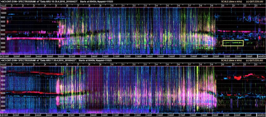
Fig. 2. (a) A 3-hour sample (01:00 to 03:00 hr) from the 24-hour long-duration false-color (LDFC)
spectrogram of Site A, 21 April 2016. (b) A 7-second portion of standard grey-scale spectrogram
extracted from the same period. The vertical axis (0–8 kHz) is the same for both spectrograms. The grey-
scale spectrogram illustrates three ‘kickee-doo’ calls of the Black Rail. These can be identified in the long-
duration false-color (LDFC) spectrogram within the yellow rectangle. The horizontal axis (x-axis) in the
left spectrogram spans three hours; in the right spectrogram, seven seconds.
Building and testing the regression call recognizer involved five recording. We implemented three recognizers using the open
steps: source WEKA Machine Learning software (Frank et al.
2016): Multilayer Perceptron, SMOreg (a regression
1. Labelling recording segments: Two complete days of
implementation of a support vector machine), and Random
recording from Site A (21 April 2016 and 23 April 2016)
Forest, all with default parameters. The support vector
were labeled at one-minute resolution (1,440 minutes for
machine and Random Forest performed equally well and
each day), each minute annotated with the number of Black
better than the Perceptron. However, the support vector
Rail calls in that minute. To determine the actual number of
machine in regression mode took approximately ten times
calls per minute, one of us (E. Znidersic, whose area of
longer to train, thus we present results only for Random
expertise is marsh birds) used a combined approach of
Forest.
visually examining standard grey-scale spectrograms and
aurally reviewing the audio recordings to count the calls. 4. Optimising the feature set: We used 10-fold cross-validation
The 1,440 minutes of 21 April 2016 included 270 minutes performance to optimize the feature set. The dominant
containing one or more Black Rail calls. The remaining components of the Black Rail call lie between 1000-3000 Hz
minutes contained zero calls. The 1,440 minutes of 23 April (Fig. 2) which includes 46 frequency bins. However,
2016 included 248 minutes containing one or more calls. including additional frequency bins on either side improved
Black Rail calls occurred during day and night of both days. performance and the final feature set consisted of 159
The 21 April recording was used for training purposes and features, 53 from each of the ACI, ENT, and EVN indices.
the 23 April recording for testing.
5. Determining performance on the test set: We assessed
2. Preparing datasets: Selecting a training set required careful performance on a previously unseen test set by applying the
consideration. A single Black Rail call has a duration of less trained recognizer to the 1,440 one-minute instances
than one second, but the acoustic features were extracted at recorded on 23 April 2016. 1192 instances contained zero
one-minute resolution. There were many minutes when calls and 248 instances contained from 1 up to a maximum
other bird species were calling in the same frequency band of 31 calls. In addition, the recognizer was applied to all
as the Black Rail and the inclusion of these minutes for recordings from Site A and Site B from 20 April 2016 to 30
training purposes would have confounded the recognizer. April 2016.
We therefore selected for training purposes, only those
minutes in the 21 April 2016 recordings where Black Rail RESULTS
calls were the dominant acoustic component in its frequency
band. The resulting training set consisted of 1,301 instances Identification of Black Rail calls in
(an instance is a one-minute segment of recording), spectrograms
including 1,170 (90%) instances containing zero calls and We collected approximately 480 hours of continuous acoustic
131 (10%) instances containing up to 18 calls. recording from the two sites (A and B) with two acoustic sensors
3. Training the recognizer: The annotated data were used to running simultaneously on the Yawkey Wildlife Center from 20
train a Random Forest recognizer for the regression task of April to 30 April 2016. It was not possible to review such a large
predicting the number of Black Rail calls in each minute of amount of data using grey-scale spectrograms at the standardAvian Conservation and Ecology 16(1): 9
http://www.ace-eco.org/vol16/iss1/art9/
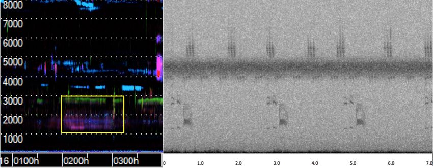
Fig. 3. Prediction of Black Rail calls by the Random Forest (RF) recognizer, trained on positive “clean” instances only. Black line =
actual counts; Red line = predicted counts. X-axis is one day from midnight to midnight and the Y-axis is the number of Black Rail
calls per minute. Note that the “clean” positives occur after 19:50 hr, and the recognizer failed to predict Black Rail calls when it was
windy or when other birds were vocalizing.
30-60 second timescale. Instead we searched all 20 LDFC When used operationally, the predictions of a recognizer are
spectrograms looking for potential Black Rail "kickee-doo" traces typically ordered from highest prediction score to lowest, and they
in the 1.5-3.0 kHz frequency band. These were then checked are verified in order until the level of false-positive predictions
against standard grey-scale spectrograms of the same one-minute becomes unacceptably high. We show the results of this approach
instances (both aurally and visually) (Fig. 2b) and with practice in Table 1, where the predictions are grouped into ranked blocks
it was possible to recognize "kickee-doo" calls in LDFC of 25, with the number of false-positive predictions per block of
spectrograms. They appear as a green line just below 3.0 kHz and 25 shown in the right-most column. A false-positive in this context
the pink/mauve color around the 1.5 kHz frequency (Fig. 2a). In is a one-minute instance that is predicted to contain at least one
general, however, it should be noted that the appearance of bird Black Rail call but contains zero calls. There were eight false-
calls in a false-color spectrogram (that is, their color and positive predictions in the first 100 ranked predictions (precision
saturation) will vary depending on the number of calls per minute, = 92%, where precision is defined as TP/(TP+FP)) and a total of
their amplitude, and of course the variability of the call. 25 in the first 150 predictions (precision = 83%). The graph of
predicted call counts over 24 hours (Fig. 3) indicates that
Performance of the call recognizer on the predictions at or below a threshold of three calls per minute are
test-day recordings unreliable and that this is a suitable cut-off point. This threshold
We compared the predicted versus actual calls per minute on the was reached at the 120th ranked prediction (Table 1), at which
test recording from 23 April 2016 at Site A (Fig. 3). The closest point there were accumulated 14 false-positive errors. The first
correlation between actual and predicted calls occurred between 120 predictions also included two correct predictions in the early
1950 hours and 2300 hours where Black Rail calls were the morning "windy" part of the day. The confounding species in the
dominant acoustic activity in its bandwidth. By comparison, the bird chorus was primarily Chuck-will’s-widow (Antrostomus
recognizer performed poorly during an interval of windy carolinensis), whose call lies in the 1.2-2.5 kHz frequency band).
conditions from 0050 hours to 0540 hours and when other birds To determine the recall (defined as TP/(TP+FN)) of the
were chorusing (from 1750 hours to 1950 hours). This result was regression recognizer, we defined a false-negative as occurring
not unexpected because we trained the Random Forest recognizer when the regression score for a one-minute instance was 3.0 or
only on positive ("clean") instances where the Black Rail call was below and the minute contained one or more calls. As noted above,
dominant in its frequency band. we considered three calls per minute as a threshold below which
The actual calling rate of Black Rail was higher during periods the recognizer would not be expected to perform accurately. Of
of wind or when other species were calling - up to 31 calls per the 248 minutes containing at least one Black Rail call, 106 were
minute as at 0530 and 1925 hours (Fig. 3). When there was little correctly predicted. Thirty-four of the false-negative predictions
other acoustic activity in the Black Rail frequency band, the were obtained from minutes containing three or fewer actual calls
maximum number of calls per minute reduced to a maximum of (Table 2). The remaining false-negative predictions could be
14 (2100 hour) (Fig.3). accounted for by the presence of additional acoustic sources inAvian Conservation and Ecology 16(1): 9
http://www.ace-eco.org/vol16/iss1/art9/
the 1-3 kHz band, for example wind, other bird species, and was no correlation between the scores for Sites A and B by plotting
anthropogenic noise (Table 2). the predictions for Sites A and B when ranked by the Site A
prediction score (Fig. 4). The LDFC spectrograms for the two
Table 1. Random Forest (RF) recognizer results from the test day sites on the test day (23 April 2016) are shown in Figure 1. A
23 April 2016, Site A. Predicted call counts were ranked from concentration of actual Black Rail calls is shown enclosed in the
highest to lowest and compared with actual counts. The number yellow rectangle in the top LDFC spectrogram for Site A. A
of false-positive predictions are shown in blocks of 25 for the top corresponding trace does not occur at the same time in the LDFC
150 ranked predictions. A false-positive in this context is a one- spectrogram for Site B.
minute instance that is predicted to contain at least one Black Rail
call but contains zero calls. Table 3. Random Forest (RF) recognizer results from the 21–30
April 2016 for Site A (316 instances) and Site B (84 instances).
Prediction Rank Prediction scores Number of false- Predicted call counts were ranked from highest to lowest and
positive predictions compared with actual counts for the top predictions at each site
1-25 9.03-7.09 0 above the call prediction threshold of 4.0.
26-50 7.08-5.81 2
51-75 5.74-4.66 1 Prediction Site A. Site A. Site B. Site B.
76-100 4.53-3.89 5 Rank Prediction False- Prediction False -
101-125 3.87-2.79 8 scores positives scores positives
126-150 2.77-2.28 9
1-25 13.45-8.63 0 7.35-5.24 25
26-50 8.59-7.52 0 5.23-4.63 25
51-75 7.51-7.05 0 4.63-4.22 25
76-84 7.04-6.89 0 4.2-4.01 9
Table 2. The number of true-positive and false-negative 84-100 6.85-6.54 2 n/a n/a
predictions for Black Rail calls on the test day, 23 April 2016, Site 100-125 6.52-6.08 1 n/a n/a
A. A false-negative in this context is a one-minute instance that 125-150 6.04-5.66 2 n/a n/a
receives a prediction score ofAvian Conservation and Ecology 16(1): 9
http://www.ace-eco.org/vol16/iss1/art9/
trade-offs between costs and benefits. The increasing popularity broad appreciation of the soundscape variability and the
of passive acoustic monitoring is due to its efficiency — greatly vocalizing species contributing to the recording. Only when major
increased effort (actual recorded time saved to SD cards) at greatly features in an LDFC spectrogram and their variability are
reduced cost (time spent by trained staff in the field). Increased understood, should attention be turned to the less obvious
effort is a desirable feature when monitoring a cryptic species such features that may reveal a rare or cryptic species such as Black
as the Black Rail, which has an irregular calling behavior (Legare Rail.
et al. 1999). Conway et al. (2004) demonstrated that an effort of
It is worth noting that a major difficulty in problem-solving with
up to 15 call-playback survey replicates would be required to
call-recognition software (such as Song-Scope, Kaleidoscope,
attain a 90% detection probability of California Black Rail
RavenPro, and MonitoR) can be determining whether bad results
(Laterallus jamaicensis coturniculus). The requirement for such
are due to incorrect use of the software or whether the acoustic
high survey effort is usually associated with greatly increased time
feature set used by the recognizer is inappropriate for the call of
in the field (Thomas and Marques 2012) and increased risk of
interest. An advantage of using LDFC spectrograms in
incorrectly inferring "absence".
conjunction with machine-learning is that, if one can visualize
the call of interest in an LDFC spectrogram, then the underlying
Fig. 4. The Black Rail prediction scores for Site A (gray) and acoustic indices offer a useful set of acoustic features that can be
Site B (red) when ranked by the first 83 Site A prediction used for machine-learning purposes.
scores. Site B predictions indicate no correlation for the same
minute. Black Rail calls were not detected by the recognizer on Before training the recognizer for this study, we made an
the dataset collected from Site B. important decision involving a cost-benefit trade-off, namely, to
train the recognizer on a regression task (predict the number of
calls per minute) rather than the usual binary classification task
(predict presence/absence of a single call). Three difficult
questions must be answered when preparing a dataset for the
binary classification task: 1. how to determine the boundaries
when cutting out individual calls, 2. how to decide which calls to
select for training, and 3. what acoustic features to extract to
optimize classification accuracy. For the regression task in this
study, these difficulties are reduced: 1. it is easier to count calls
per minute over consecutive non-overlapping minutes, 2. all calls
are counted, and 3. the feature set was the same as that used to
construct the LDFC spectrograms. Indeed, our ability to visualize
Black Rail calls in the LDFC spectrograms informed us that
Recognizer performance spectral indices would make suitable features for the regression
The increased efficiency of passive acoustic monitoring comes at task. The cost associated with extracting features at one-minute
a cost, namely the increased requirement for data storage and resolution was the increased probability that other acoustic events
automated analysis, both of which require computational skills would confound recognition of Black Rail calls, leading to a
that are not always part of an ecologist's training. Consequently, higher number of false-negative predictions.
cost/benefit decisions around data analysis can become an
Of the 248 test-day minutes containing at least one Black Rail
important component of monitoring decisions. As an example, a
call, 142 were not detected by the recognizer, an implied false-
machine-learned recognizer, trained to detect Black Rail calls,
negative rate of 57%. An analysis of these 142 minutes revealed
yielded only 91 true positives from 11,872 predictions for a
that 108 were due to the confounding presence of other acoustic
precision of 0.77% (Bobay et al. 2018). In this case, cost saving in
sources and 34 were due to the actual call rate being below 3 calls
the field was offset by the cost of processing a large volume of
per minute where recognizer performance was unreliable. A
recognizer output. As these authors note, the inability to achieve
weakness of working at one-minute resolution is that our method
accurate analysis of acoustic data can deter ecologists from
only detects Black Rail calls in those minutes where they are
applying passive acoustic monitoring.
dominant in their frequency band. However, when this condition
Generally, more acoustic data is collected than can be listened to was satisfied, the false-negative rate was 14% (34/248, the fraction
or visually reviewed, so the standard approach is to train a of calling minutes below 4 calls per minute).
recognizer to detect vocalizations of the target species. Besides
A question arises concerning lack of detection of Black Rail calls
the possible software costs and time required to learn the software,
at Site B and whether a call recognizer trained on recordings from
there are additional significant time costs in assembling labeled
Site A would be reliable when analyzing recordings from Site B.
datasets and verifying recognizer performance. These latter costs
As a rule-of-thumb, the training, validation, and test sets that
should not be underestimated and the old adage, "rubbish in -
determine the performance of a machine-learned model should
rubbish out", is worth keeping in mind.
be representative of the intended operational environment. Sites
The ability to visualize our 20 days of recording in 20 LDFC A and B were 490 meters apart and acoustically isolated. However,
spectrograms was an important contribution to the success of this they were within the same impounded marsh and had the same
monitoring exercise. The alternative would have been to review vegetation composition and structure. Therefore, we are confident
28,800 standard scale spectrograms of one-minute duration. that sites A and B were sufficiently similar both acoustically and
Interpreting LDFC spectrograms requires the ecologist to have a biologically, that Black Rail would have been detected during the
10-day deployment if it had been present.Avian Conservation and Ecology 16(1): 9
http://www.ace-eco.org/vol16/iss1/art9/
We conclude that the recognizer prediction error rates are within to or scanned with standard scale spectrograms) and to detect
acceptable bounds subject to two important conditions: 1. the Black Rail calls. The technical difficulty in implementing our
target bird species is the dominant sound source in its frequency method is only moderate. The software used to calculate acoustic
band in some of its calling minutes; and 2. the field recordings indices and prepare LDFC spectrograms is a command-line tool
have sufficient spatial and temporal cover to detect target calls if but does not require any coding. WEKA is a well-known machine-
they occur. This brings us to the issue of spatial cover and survey learning toolkit with extensive documentation. As an alternative,
point placement. R or Python could be used to do the machine learning step.
However, it will always remain the case that a trade-off exists
Survey point placement between the time it takes to perform a task manually and the time
Incorrectly inferring absence is a critical issue with all monitoring it takes to prepare the automation of the task.
methods (Kéry 2002). Such errors can have serious management
This approach has been applied to other marsh bird species
consequences, especially for threatened species (Robinson et al.
(Znidersic et al. 2020; Towsey et al. 2018b) and can be applied to
2018) such as the Black Rail. Although acoustic monitoring
other taxa where the primary mode of detection is auditory, and
satisfies some efficiency criteria, budget constraints will demand
it is cost and time effective to apply a semi-automated analytical
consideration of additional effectiveness/efficiency trade-offs
approach. Consideration still must be given to the species of
(Joseph et al. 2006), particularly those concerning spatial and
interest, what is the best monitoring method for detection and the
temporal placement of recorders in the field.
availability of time and budget. In addition, there is the ethical
Sample point spacing (for either passive acoustic monitoring or consideration. As ecologists, we must reduce our impacts on the
call-playback surveys) is critical to detection probability and environment and species by working smarter with the use of
therefore, should not be compromised to increase large scale technology. As we know so little about the effects of call-playback
spatial coverage. Although marginally outside the guidelines for and bird call apps on species and communities (Johnson and
call-playback surveys of marsh birds (Conway 2011), in our study, Maness 2018, Watson et al. 2018), the application of passive, low
the two acoustic sensors were 490 m apart which resulted in impact monitoring methods should lead future investigations.
significant variation in detection of Black Rail between the two
Our results imply that improvements can be made to both on-
sites. If detection was based purely at Site B, instead of Site A,
ground monitoring (passive acoustic monitoring and call-
there is a high probability that Black Rail would not have been
playback surveys) of Black Rail and the subsequent analysis of
detected either from a call-playback survey or by reviewing
acoustic data. Passive acoustic monitoring has the capability to
acoustic recordings. Therefore, the closer the sampling points, the
collect large-scale temporal and spatial data, therefore increasing
lower the risk of incorrectly inferring absence. (Conway 2011,
detection probability of this secretive species. The vocalization
Schroeder and McRae 2019).
behavior of the Black Rail is not consistent, seemingly affected
Vocalization strategies by weather (wind and rain) and the vocalization of other species
We also found that Black Rail called during only four consecutive in the same frequency band. Therefore, a standard monitoring
days of the ten-day recording. This may be attributed to the protocol would need to be approached with some flexibility
variation of specific vocalization strategies (such as the "kickee- including timing and duration of passive acoustic monitoring,
doo" call) or movement within territories during the breeding and the acoustic recorder placement. We see the potential for
period (Conway et al. 2004). If our recording duration had been future work to include multiple agencies combining datasets to
reduced to just a few days on the assumption that, if a Black Rail further refine the training of Black Rail recognizers using this
was present, it would call at some time during the day, our result method. This would result in a more scalable and transferable
would have been a false-negative. approach to detecting and monitoring Black Rail, therefore
informing better decision making about where and when to
Long-duration recordings offer the possibility of noting monitor.
unexpected behavioral observations. For example, assumed
vocalization patterns may only be dependent upon environmental We recommend individual site assessment taking into
conditions (wind and rain) or vocalizations of other species within consideration spatial placement of passive acoustic recorders
frequency bands. In the case of Black Rail, the calling rate according to potential sound attenuation influences (Yip et al.
increased when the conditions were windy or there were 2017). Also, vocalization intensity may be associated with
competing species in the frequency band (maximum call rate of breeding stage (Legare et al. 1999). Therefore, frequency of
31 per minute). This compares to a maximum calling rate of 14 survey, whether passive acoustic monitoring or call-playback
calls per minute during the quiet time. survey, should be increased during the breeding season.
Large datasets generated by long-duration passive acoustic
Conclusion and prospect monitoring require semi-automated analytical techniques such as
Our study has demonstrated that the high sampling effort required call recognition. Solid data management protocols are also
to detect Black Rail, or to more confidently infer its absence, can required to ensure data are available for further and future analysis
be achieved efficiently using long-duration recordings from as analytical tools improve.
passive acoustic monitoring. Although this was a comparatively
small study consisting of just two sites, we have demonstrated that The machine learning approach which we have described offers
our method of combining two semi-automated analytical tools a middle path between simple but brittle, hand-crafted templates
(LDFC spectrograms and the regression call-recognizer) was able and the great complexity of convolution neural networks that
to process a large-dataset (far more audio than could be listened require very large-training sets for deep-learning (PriyadarshaniAvian Conservation and Ecology 16(1): 9
http://www.ace-eco.org/vol16/iss1/art9/
2018). These are simply not available for a rare, cryptic species. species detectability on volunteer based anuran monitoring
Therefore, we recommend long-duration false-color spectrograms programs. Biological Conservation 121:585-594. https://doi.
and a call recognizer to analyze Black Rail datasets, applying both org/10.1016/j.biocon.2004.06.018
visual and machine learning features. Although both tools have
Drake, K. L., M. Frey, D. Hogan, and R. Hedley. 2016. Using
their limitations, these are compensated by high monitoring effort
digital recordings and sonogram analysis to obtain counts of
and relative ease in preparing a call recognizer.
yellow rails. Wildlife Society Bulletin 40(2):346-354. https://doi.
org/10.1002/wsb.658
Responses to this article can be read online at: Eddleman, W. R., R. E. Flores, and M. Legare. 2020. Black Rail
https://www.ace-eco.org/issues/responses.php/1773 (Laterallus jamaicensis) in The Birds of The World Online (A.
Poole and F. B. Gill, Eds.). Cornell Lab of Ornithology, Ithaca,
New York. https://doi.org/10.2173/bow.blkrai.01
Acknowledgments: Estrada-Villegas, S., C. F. J. Meyer, and E. K. V. Kalko. 2010.
Effects of tropical forest fragmentation on aerial insectivorous
Thanks to the staff at the South Carolina Department of Natural
bats in a land-bridge island system. Biological Conservation
Resources at Yawkey Wildlife Center particularly J. Dozier and J.
143:597-608. https://doi.org/10.1016/j.biocon.2009.11.009
Lee for providing access, accommodation and logistical support.
Also thanks to field technicians K. Brunk and S. Apgar. Fischer, F. P., U. Schulz, H. Schubert, P. Knapp, and M. Schmöger.
1997. Quantitative assessment of grassland quality: acoustic
determination of population sizes of Orthopteran indicator
LITERATURE CITED species. Ecological Applications 7:909-920. https://doi.
Bibby, C. J., N. D. Burgess, and D. A Hill. 1992. Bird census org/10.1890/1051-0761(1997)007[0909:QAOGQA]2.0.CO;2
techniques. Academic Press Limited, San Diego, California. Frank, E., M. A. Hall and I. H. Witten. 2016. The WEKA
Bioacoustics Research Program. 2014. Raven Pro: Interactive Workbench. Online Appendix for "Data Mining: Practical Machine
Sound Analysis Software (Version 1.5) Computer software. Ithaca, Learning Tools and Techniques". Morgan Kaufmann, Fourth
NY: The Cornell Lab of Ornithology. [online] URL: http://www. Edition.
birds.cornell.edu/raven. Gu, W., and R. K. Swihart. 2003. Absent or undetected? Effects
Bobay, L. R., P. J., Taillie, and C. E. Moorman. 2018. Use of of non-detection of species occurence on wildlife-habitat models.
autonomous recording units increased detection of a secretive Biological Conservation 116:195-203. https://doi.org/10.1016/
marsh bird. Journal of Field Ornithology 89:384-392. https://doi. S0006-3207(03)00190-3
org/10.1111/jofo.12274 Johnson. J. M., and T. J. Maness. 2018. Response of wintering
Charif, R. A., A. M. Waack, and L. M. Strickman. 2008. Raven birds to simulated birder playback and phishing. Journal of the
Pro 1.3 user's manual. Cornell Laboratory of Ornithology, Ithica, Southeastern Association of Fish and Wildlife Agencies 5:136-143.
New York.
Joseph, L. N., S. A. Field, Wilcox, C., and H. P. Possingham. 2006.
Collier, T. C., D. T. Blumstein, L. Girod, and C. E. Taylor. 2010. Presence-Absence versus abundance data for monitoring
Is alarm calling risky? Marmots avoid calling from risky places. threatened species. Conservation Biology 20:1679-1687. https://
Ethology 116:1171-1178. https://doi.org/10.1111/j.1439-0310.2010.01830. doi.org/10.1111/j.1523-1739.2006.00529.x
x
Kéry, M. 2002. Inferring the absence of a species: A case study
Conway, C. J. 2011. Standardized North American marsh bird of snakes. Journal of Wildlife Management 66:330-338. https://
monitoring protocol. Waterbirds 34:319-346. https://doi. doi.org/10.2307/3803165
org/10.1675/063.034.0307
Legare, M. L., W. R. Eddleman, P. A. Buckley, and C. Kelly. 1999.
Conway, C. J., C. Sulzman, and B. E. Raulston. 2004. Factors The Effectiveness of Tape Playback in Estimating Black Rail
affecting detection probability of California Black rails. Journal Density. The Journal of Wildlife Management 63:116-125. https://
of Wildlife Management 68:360-370. https://doi.org/10.2193/0022-541X doi.org/10.2307/3802492
(2004)068[0360:FADPOC]2.0.CO;2
Legare, M. L., and W. R. Eddleman. 2001. Home range size, nest-
Crouch, W. B. III, and P. W.C. Paton. 2002. Assessing the use of site selection and nesting success of black rails in Florida. Journal
call surveys to monitor breeding anurans in Rhode Island. Journal of Field Ornithology 72:170-177. https://doi.org/10.1648/0273-8
of Herpetology 36:185-192. https://doi.org/10.1670/0022-1511 570-72.1.170
(2002)036[0185:ATUOCS]2.0.CO;2
Lieury, N., S. Devillard, A. Besnard, O. Gimenez, O. Hameau, C.
Davidson, L. M. 1992. Black Rail. Pages 119-134 in K. J. Ponchon, and A. Millon. 2017. Designing cost-effective capture-
Schneider and D. M. Pence (eds), Migratory non-game birds of recapture surveys for improving the monitoring of survival in bird
management concern in Northeast. U.S Fish and Wildlife Service, populations. Biological Conservation 214:233-241. https://doi.
Newton Corner, Massachusetts, USA. org/10.1016/j.biocon.2017.08.011
de Solla, S. R., L. J., Shirose, K. J., Fernie, G. C., Barrett, C. S., Linke, S., T. Gifford, C. Desjonquères, D. Tonolla, T. Aubin, L.
Brousseau, and C. A. Bishop. 2005. Effect of sampling effort and Barclay, C. Karaconstantis, M. J. Kennard, F. Rybak, and J. Sueur.Avian Conservation and Ecology 16(1): 9
http://www.ace-eco.org/vol16/iss1/art9/
2018. Freshwater ecoacoustics as a tool for continuous ecosystem Sueur, J., S. Pavoine, O. Hamerlynck, and S. Duvail. 2008. Rapid
monitoring. Frontiers in Ecology and the Environment 16:231-238. acoustic survey for biodiversity appraisal. PLOS ONE, 3, e4065.
https://doi.org/10.1002/fee.1779 https://doi.org/10.1371/journal.pone.0004065
Parmentier, E., L. Di Iorio, M. Picciulin, S. Malavasi, J. P. Thomas, L., and T.A. Marques. 2012. Passive acoustic monitoring
Lagardere, and F. Bertucci. 2018. Consistency of spatiotemporal for estimating animal density. Acoustics Today 8:35-44. https://
sound features supports the use of passive acoustics for long-term doi.org/10.1121/1.4753915
monitoring. Animal Conservation 21:211-220. https://doi.
Towsey, M. 2017. The calculation of acoustic indices derived from
org/10.1111/acv.12362
long-duration recordings of the natural environment. [online]
Pellet, J., and B. R. Schmidt. 2005. Monitoring distributions using URL: https://eprints.qut.edu.au/110634
call surveys: estimating site occupancy, detection probabilities
Towsey, M., A. Truskinger, M. Cottman-Fields, and P. Roe. 2018a.
and inferring absence. Biological Conservation 123:27-35. https://
Ecoacoustics Audio Analysis Software v18.03.0.41 (Version
doi.org/10.1016/j.biocon.2004.10.005
v18.03.0.41). Zenodo. [online] URL: http://doi.org/10.5281/
Peterson, S. M., H. M. Streby, J. A. Lehman, G. R. Kramer, A. zenodo.1188744
C. Fish, and D. E. Anderson. 2015. High-tech or field techs:
Towsey, M, L. Zhang, M. Cottman-Fields, J. Wimmer, J. Zhang,
Radio-telemetry is a cost-effective method for reducing bias in
and P. Roe. 2014 ‘Visualization of long-duration acoustic
songbird nest searching. The Condor 117:386-396. https://doi.
recordings of the environment’, Procedia Computer Science, vol.
org/10.1650/CONDOR-14-124.1
29, pp. 703-712
Pieretti, N., A. Farina, and D. Morri. 2011. A new methodology
Towsey, M., E. Znidersic, J. Broken-Brow, K. Indraswari, D. M.
to infer the singing activity of an avian community: The Acoustic
Watson, Y. Phillips, A. Truskinger, and P. Roe. 2018b. Long-
Complexity Index (ACI). Ecological Indicators 11:868-873.
duration, false-colour spectrograms for detecting species in large
https://doi.org/10.1016/j.ecolind.2010.11.005
audio datasets. Journal of Ecoacoustics 2: #IUSWUI. https://doi.
Priyadarshani, N., S. Marsland and I. Castro. 2018. Automated org/10.22261/jea.iuswui
birdsong recognition in complex acoustic environments: a review.
U.S. Fish and Wildlife Service. 2020. Petition finding and proposed
Journal of Avian Biology 49:jav-01447 https://doi.org/10.1111/
threatened species status for Eastern Black Rail with a 4(d) rule.
jav.01447
[online] URL: https://www.federalregister.gov/documents/2020/
Robbins, C. S., B. Brown and H. S. Zim. 1983. A guide to field 10/08/2020-19661/endangered-and-threatened-wildlife-and-plants-
identification: birds of North America. Golden Press, New York, threatened-species-status-for-eastern-black-rail-with
New York.
Watson, D. M. 2017. Sampling effort determination in bird
Robinson, N. M., B. C. Scheele, S. Legge, D. M. Southwell, O. surveys: do current norms meet best-practice recommendations?
Carter, M. Lintermans, J. Q. Radford, A. Skroblin, C. R. Wildlife Research 44:183-193. https://doi.org/10.1071/WR16226
Dickman, J. Koleck, A. F. Wayne, J. Kanowski, G. R. Gillespie,
Watson, D. M., E. Znidersic, and M. Craig. 2018. Ethical birding
D. B. Lindenmayer. 2018. How to ensure threatened species
call playback and conservation. Conservation Biology 33:469-471.
monitoring leads to threatened species conservation. Ecological
https://doi.org/10.1111/cobi.13199
Management and Restoration 19:222-229. https://doi.org/10.1111/
emr.12335 Weske, J. S. 1969. An ecological study of the Black Rail in
Dorchester County, Maryland. Thesis, Cornell University, USA.
Schroeder, K. M, and S. B. McRae. 2019. Vocal repertoire of the
King Rail (Rallus elegans). Waterbirds 42(2):154-167. https://doi. Wildlife Acoustics. 2017. 4.3.1 Documentation. [online] URL:
org/10.1675/063.042.0202 https://www.wildlifeacoustics.com/images/documentation/Kaleidoscope.
pdf (accessed 19 January 2019).
Sidie-Slettedahl, A. M., K. C. Jensen, R. R. Johnson, T. W.
Arnold, J. E. Austin, and J. D. Stafford. 2015. Evaluation of Yip, D. A., E. M. Bayne, P. Solymos, J. Campbell, and D. Proppe.
autonomous recording units for detecting 3 species of secretive 2017. Sound attenuation in forest and roadside environments:
marsh birds. Wildlife Society Bulletin 39:626-634. https://doi. Implications for avian point-count surveys. The Condor
org/10.1002/wsb.569 119:73-85. https://doi.org/10.1650/CONDOR-16-93.1
Sousa-Lima, R. S., T. F. Norris, J. N. Oswald, and D. P. Fernandes. Znidersic, E., M. Towsey, W. K. Roy, S. E. Darling, A. Truskinger,
2013. A review and inventory of fixed autonomous recorders for P. Roe, and D. Watson. 2020. Using visualization and machine
passive acoustic monitoring of marine mammals. Aquatic learning methods to monitor low detectability species-- The least
Mammals 39:205-210. https://doi.org/10.1578/AM.39.2.2013.205 bittern as a case study. Ecological Informatics, 55,101014. https://
doi.org/10.1016/j.ecoinf.2019.101014
Editor-in-Chief: Alexander L.Bond
Subject Editor: Steven L.Van WilgenburgYou can also read