Depression alters the circadian pattern of online activity - Nature
←
→
Page content transcription
If your browser does not render page correctly, please read the page content below
www.nature.com/scientificreports
OPEN Depression alters the circadian
pattern of online activity
Marijn ten Thij1*, Krishna Bathina1, Lauren A. Rutter2, Lorenzo Lorenzo‑Luaces2,
Ingrid A. van de Leemput3, Marten Scheffer3 & Johan Bollen1,3
Human sleep/wake cycles follow a stable circadian rhythm associated with hormonal, emotional,
and cognitive changes. Changes of this cycle are implicated in many mental health concerns. In fact,
the bidirectional relation between major depressive disorder and sleep has been well-documented.
Despite a clear link between sleep disturbances and subsequent disturbances in mood, it is difficult
to determine from self-reported data which specific changes of the sleep/wake cycle play the most
important role in this association. Here we observe marked changes of activity cycles in millions of
twitter posts of 688 subjects who explicitly stated in unequivocal terms that they had received a
(clinical) diagnosis of depression as compared to the activity cycles of a large control group (n = 8791).
Rather than a phase-shift, as reported in other work, we find significant changes of activity levels in
the evening and before dawn. Compared to the control group, depressed subjects were significantly
more active from 7 PM to midnight and less active from 3 to 6 AM. Content analysis of tweets
revealed a steady rise in rumination and emotional content from midnight to dawn among depressed
individuals. These results suggest that diagnosis and treatment of depression may focus on modifying
the timing of activity, reducing rumination, and decreasing social media use at specific hours of the
day.
Depression is one of the most important global public health challenges. It is the single largest contributor to dis-
ability and disease, affecting 4% of the world’s population, causing 11% of all years lived with disability globally1.
It is furthermore associated with a reported 800,000 suicides on an annual basis, mostly among young a dults2.
Depression is significantly under-reported, under-diagnosed, and under-treated, in part due to its heterogeneous
nature which involves subjective and culturally shaped experiences such as motivation, mood, and well-being3.
Furthermore, in spite of its prevalence, the dynamics of its onset and development remain poorly understood4–6,
limiting the development of treatment o ptions7,8.
Like most mammals9, humans experience circadian rhythms involving hormonal, behavioral, and cognitive
changes that lead to stable sleep-wake cycles, even when individuals are disconnected from natural d aylight10,11 or
travel across time zones. Unsurprisingly, a stable daily activity cycle is important to maintain physical and mental
health12,13. In fact, disturbances of the human circadian rhythm are strongly associated with mood d isorders14–22
such as depression and anxiety, bipolar, and borderline personality disorder. The severity of depression has
been linked to the magnitude of the sleep-wake cycle d isturbance23 while reports of sleep disturbances can be
used as an early warning signal of recurrent depression24 and predict risk of poor outcomes in treatments for
depression25. As a result, interventions targeting sleep are now considered an essential component of efforts to
improve depression treatment outcomes26,27. This is also emphasized by the central position of sleep-related
symptoms in disorder n etworks28.
Although the connection between sleep-wake cycle disturbances and depression has been firmly established,
it is not clear which specific disturbances or changes are most strongly implicated in the onset and remission of
depression. Reports of the effectiveness of sleep deprivation t herapy29,30 indicate that the association between
sleep and mood disorders is not necessarily modulated by the amount of sleep per s e31, but by its specific timing
and pattern. In particular, questions have arisen with respect to whether phase and/or magnitude changes of the
sleep-wake cycle account for the association between sleep and risk for depression32.
Observations of daily activity levels of individuals require continuous monitoring of a large number of sub-
jects throughout numerous circadian cycles to establish sufficient statistical power while avoiding observer
bias. However, most studies establishing circadian rhythm disturbances in mental disorders suffer from small
sample sizes33. These limitations can be mitigated by the post hoc analysis of alternative sources of information
1
Luddy School of Informatics, Computing and Engineering, Center for Social and Biomedical Complexity, Indiana
University Bloomington, Bloomington, IN 47408, USA. 2Department of Psychological and Brain Sciences, Indiana
University Bloomington, Bloomington, IN 47405, USA. 3Aquatic Ecology and Water Quality Management,
Wageningen University, Wageningen 6708 PB, The Netherlands. *email: mtenthij@indiana.edu
Scientific Reports | (2020) 10:17272 | https://doi.org/10.1038/s41598-020-74314-3 1
Vol.:(0123456789)www.nature.com/scientificreports/
“Depressed” cohort “Random” cohort
All individuals 688 8791
Male 181 3313
Gender
Female 356 2,918
18 and under 31 613
19–29 78 659
Age
30–39 58 538
40 and over 41 1,006
Table 1. Demographic information derived with M345 for both cohorts.
such as microblogs, diaries, mobile phone34, and social media activity. The latter in particular serve as a daily
cognitive and behavioral diary to billions of individuals. In fact, activity levels in on-line platforms, e.g. using
Digg35, Foursquare36, Twitter37, Wikipedia editing b ehavior38, and Y
ouTube35, have already proven to be a useful
resource to estimate circadian cycles.
Here, we use large-scale, longitudinal, social media activity data to study the daily activity cycles of hundreds
of individuals who stated in unequivocal terms that they had received a (clinical) diagnosis of depression, using
an similar sample inclusion criterion as Coppersmith, Dredze & Harman39. We find that the activity levels of
depressed individuals, like those of a random sample, fluctuate reliably according to a well-defined circadian
rhythm as was shown previously40. Our results extend these findings by showing no evidence of a significant
phase-shift, but rather that activity levels for the depressed individuals differ significantly in the early evening
and early morning hours, which is when we also see increased indications of emotionality and self-reflection.
These findings point towards targeted interventions that focus on the reduction of rumination at specific times
of the day.
Cohort definition
For our analysis, we define 2 disjoint cohorts of Twitter users: “Depressed” and “Random”. In our “Depressed”
cohort we only include individuals with a (clinical) diagnosis of depression, which they report on Twitter explic-
itly (e.g., “Went to my doctor today and got officially diagnosed with major depression”), similar to the approach
of Coppersmith, Dredze & H arman39. A team of 3 raters independently evaluated each ‘diagnosis tweet’ to deter-
mine whether it pertained to an explicit, unequivocal statement of an actual diagnosis, removing self-diagnoses,
retweets, quotes, or jokes. In other words, we excluded individuals who “self-diagnosed” with depression. This
second step was taken to remove false-positives from the cohort, which has been proven to increase performance
in classification t asks41. We also mapped references to a time of diagnosis, e.g. “today”, “last week”, “2 months
ago”, or “in 2014” to a likely diagnosis time interval (see “Methods”). This method is akin to research on elec-
tronic health records (EHRs) as well as pharmacoepidemiological methods in the sense that we rely on reports
of an actual diagnosis but are receiving this information directly from the individual with the diagnosis. This
allows us to tie the diagnosis to their social media record, which provides indicators of their evolving mood,
cognition, language, and behavior. While the recognition of depression is poor in some s ettings42, patients who
are recognized as being depressed tend to, on average, have higher levels of depression than those who are not
recognized43. This finding, along with research suggesting depression is best understood as existing on a con-
tinuum (for a review see Ruscio44), supports the validity of our inclusion criteria for the “Depressed” cohort. We
found 688 individuals that explicitly stated their (clinical) depression diagnosis and whom we assigned to the
“Depressed” cohort, or D cohort for short. We downloaded the past tweets of these aforementioned individuals
to obtain a longitudinal timeline.
Neither the reported diagnosis nor the Twitter profiles of the sampled individuals provide demographic
information with respect to our D cohort. However, a highly accurate sex classifier45 (Macro-F1: 0.915) applied
to the Twitter profiles of our D cohort (see “Methods”), shows that it has a similar 2:1 female to male ratio as
observed in clinical studies46, indicating that the demographics of our Twitter cohort closely match previous
clinical findings. The indicated age distribution of our D cohort (though less reliable, Macro-F1: 0.425), is also
in line with clinical studies46,47, specifically we find a decreasing number of individuals per age-group as the age
of the group increases in our D cohort.
We define our “Random” cohort, or RS cohort for short, as a control group by taking a random sample of
8791 Twitter users. To compensate for possible changes of user behavior in the social media platform over
time, we sample these individuals such that the distribution of their account creation month matches that of
the individuals in the D cohort (see Supplementary Information Section 2). Table 1 describes the demographic
information obtained for both cohorts.
Measuring activity levels
We assume that sleeping individuals can not tweet and that we can therefore gauge changes in activity levels by
counting the number of tweets that an individual posts at a given time. Working at an hourly resolution, we count
the number of tweets that an individual has posted at a given hour of the day and divide each hourly count by
the total number of tweets for all hours of the day. This results in an hourly percentage of daily Twitter activity
for the individual (denoted Au). We can then calculate a cohort hourly activity level for either the D cohort or
Scientific Reports | (2020) 10:17272 | https://doi.org/10.1038/s41598-020-74314-3 2
Vol:.(1234567890)www.nature.com/scientificreports/
Figure 1. Bootstrapped normalized activity levels for the “Depressed” and “Random” cohorts. The markers
display the median outcome of 10,000 runs, where we use the number of individuals in each cohort as the
sample size per run (n = 688 for the “Depressed” and n = 8791 for the “Random” cohort). The solid lines
display the cubic spline fit of these hourly values. The dark and light gray shaded areas indicate the day/night
times during the cycle (see “Methods”).
the RS cohort, denoted AD or ARS , respectively, by combining all hourly counts across the individuals in the
specific cohort and dividing by the total number of tweets across these individuals. Note that we exclude retweets
and account for each individual’s local time to ensure counts pertain to the same time of day.
Naturally, differences can arise in the level of activity between both individuals and cohorts in general. Since
we are not looking to make inferences about the total amount of tweets nor the average number of tweets per
cohort, but rather the relative differences of hourly activity patterns between the two cohorts, we account for this
variation by calculating hourly activity levels for 10,000 re-samples of the individuals in the D and RS cohorts
with replacement, i.e. we bootstrap hourly activity levels for each cohort. This re-sampling results in a distribu-
tion of activity levels for each hour (each from a different sample of individuals) that can be characterized by its
median and 95% confidence interval, denoted by AD⋆ and ARS ⋆ respectively for the D and RS cohort.
Circadian activity levels
The resulting time series AD⋆ and ARS ⋆ are displayed in Fig. 1. As a reference to aid the eye, we show the times
of dawn, sunrise, sunset and dusk as gray bands. We repeat the cycle twice in Fig. 1 to better highlight the daily
variation around midnight.
For both the D and RS cohorts, we find periodic changes in activity levels throughout the day, resulting in a
well-defined circadian rhythm of activity levels. We find that both cohorts experience a valley in activity levels
from roughly 10PM to 6AM, a time that is traditionally reserved for sleep. Activity levels quickly recover from
a low point at 6AM as people wake up and become active during the morning hours. This is followed by a first
peak at noon, after which activity plateaus for 6 h from noon to 6 PM. This is followed by a slight ramp up of
activity peak around 9 PM, after which activity levels drop again.
Tweets can be posted at any time of year, hence seasonal changes in daylight times or Daylight Savings Time
could affect our observations. However, we find that daylight times changes throughout the year do not account
for our pattern of results (see Section 3.2 of the Supplementary Information).
Differences in activity levels between “Depressed” and “Random” cohorts
As shown in Fig. 1, activity levels of the D and RS cohorts follow a similar circadian rhythm with valleys and
peaks occurring at approximately the same time. We find no evidence of a phase-shift in daily activity levels; the
pattern of changes, including the valleys and peaks of the circadian rhythm, match exactly across the D and RS
time series. A cross-correlation function indicates that the Pearson correlation coefficient between the two time
series peaks exactly at a lag of zero (see Supplemental Information Section 4), providing further indication of
the absence of a phase-shift between the sleep/wake cycles of the D and RS cohorts.
However, in spite of the absence of a phase shift in Fig. 1, we do find that activity levels diverge significantly at
specific times of day between the D and RS cohorts. In particular, we find divergences from 3AM to 6AM, 9AM to
noon, and a particularly sharp divergence from 9PM to midnight. In the latter case, surprisingly, we observe that
the D cohort is approximately 1% more active than the RS cohort, a considerable amount relative to the expected
range of percentage-wise hourly fluctuations throughout the day for both cohorts, namely roughly 1% to 8%
from peak to valley and an expected 4.16% hourly activity if uniformly distributed over 24 h (100%/24 ≃ 4.16%).
To objectively determine the significance of the observed differences between the circadian activity levels of
the D and RS cohorts, we calculate the hourly relative differences of activity levels between the two cohorts, i.e.
the ratio of activity levels at hour i between the D and RS cohort. If this ratio equals 1 we assume the activity levels
are equal. Activity level ratios significantly larger or lower than 1 indicate a significant difference in activity levels.
Figure 2A shows that this relative difference is lowest at 5AM and highest at 9 PM, i.e. individuals in the D
cohort are much less active in the early morning (−27% from 3 to 6 AM) but more active in the evening (+10%
from 7 PM to midnight) compared to individuals from the RS cohort.
Our cohorts are comprised of individuals with different activity levels. It follows that the inclusion or exclu-
sion of individuals in both cohorts will affect our estimate of activity level differences. This should be taken into
account when we assess whether or not activity levels are significantly different at a particular hour between the
two cohorts. We therefore bootstrap the difference between the two activity levels (AD − ARS ), by re-sampling
Scientific Reports | (2020) 10:17272 | https://doi.org/10.1038/s41598-020-74314-3 3
Vol.:(0123456789)www.nature.com/scientificreports/
A
B
Figure 2. Bootstrapped difference between the normalized activity levels for the “Depressed” and “Random”
cohorts. (A) Relative difference between the “Depressed” and “Random” cohorts. The markers indicate the
hourly relative difference between the mean activity levels (see Fig. 1) for both cohorts and the solid black line
displays the cubic spline fit of these hourly values. (B) Bootstrapped difference between the “Depressed” and
“Random” cohorts. The diamonds display the median outcome of the difference in outcome of the 10,000 runs
and the vertical lines display the 95% CI of the difference in the bootstrap outcomes. The hours displayed in
bold indicate that there is a significant difference in behavior between the two cohorts. Furthermore, the gray
shaded areas in both panels indicate the hours in which there is a significant difference in activity and the black
dashed lines in both panels are meant as a reference lines that indicate equal behavior for both cohorts.
Figure 3. Z-score normalized relative difference in token
usage between the “Depressed” and “Random”
cohorts. The Z-score normalized hourly values of PRh Cx for all selected tokens and each category are
indicated by the colored markers (see SI Section 5 for the actual values). The solid lines display the cubic spline
fit of the hourly values. The black dashed line is a visual representation of the mean behavior. Furthermore, the
gray shaded areas indicate the hours in which there is a significant difference in activity.
the individuals in both cohorts with replacement. This results in a distribution of difference values that we
can characterize by its median and 95% confidence interval (CI), as shown in Fig. 2B. If the resulting 95% CI
does not include 0, we conclude that the activity levels for that hour differ between the D and RS cohorts at the
α < 0.05 level48.
According to this criterion, we find the following statistically significant divergence of circadian activity levels:
less activity for the D cohort between 3 and 6AM, 9 and 10AM, and 1 and 2PM, as well as more activity in the
evening between 7PM and midnight for the D cohort. These times of significant differences are also marked in
Figs. 2 and 3 by the gray shaded areas. Strikingly, the differences in the morning hours do not coincide with the
distribution of dawn or sunrise times, which we determined for the location of all individuals in each cohort
using their self-reported location information (see “Methods”). This indicates that the differences are not caused
by variances in the response to daylight hours.
Content analysis
The circadian activity levels of the D and RS cohorts differ significantly at specific times of the day. To investi-
gate the cognitive factors that may affect these differences, we analyze the content of the tweets posted by the
individuals in both cohorts at those times when activity levels diverge significantly.
Two experts in cognitive-behavioral therapy (CBT) selected a set of 76 tokens (listed in Table 2), each falling
into six different categories (denoted by Cx ) related to “self-reflection” and “rumination” (e.g. Personal Pronouns,
Scientific Reports | (2020) 10:17272 | https://doi.org/10.1038/s41598-020-74314-3 4
Vol:.(1234567890)www.nature.com/scientificreports/
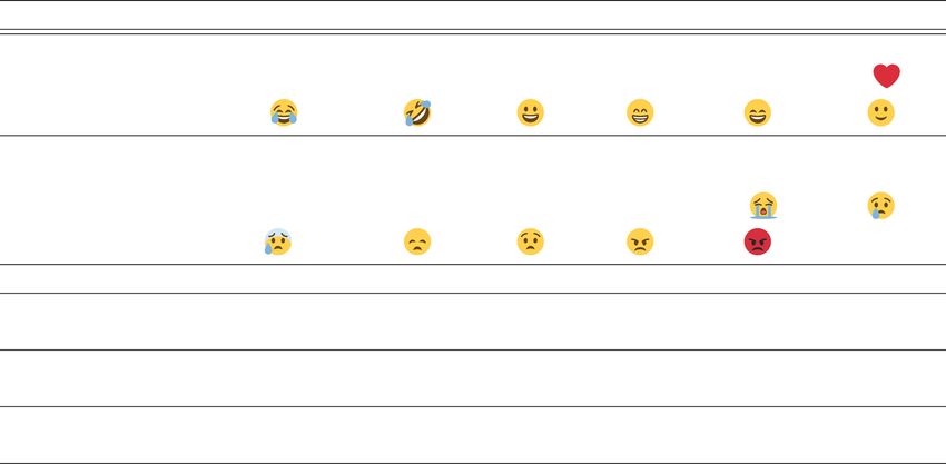
Table 2. Overview of tokens used for content analysis. An * indicates that a token was not consistently in the
top 250 tokens for each hour in both cohorts.
23
Category (Cx) Prevalence ratio ( PR(Cx )) Hourly prevalence ratio ( 24
1
h=0 PRh (Cx ))
All selected tokens 1.4885 1.5279
Personal pronouns 1.7601 1.8217
Positive affect 1.4593 1.4589
Negative affect 1.6982 1.7666
Rumination 1.2455 1.2836
Questioning 1.2319 1.2618
Rigid thinking 1.3467 1.3922
Table 3. Prevalence ratios in token use for all considered categories.
where x = PP so CPP ), with a set of tokens expressing “positive affect” as a control. We define the prevalence
of a token t in a cohort (i.e., D for “Depressed” or RS for “Random”) as the expected number of times that the
token is used per tweet (denoted by fD (t) and fRS (t), respectively). The first column of Table 3 shows that the
token prevalence ratio between the D and RS cohorts for all considered categories (denoted by PR(Cx )) is much
larger than 1.
Like our activity level time series, we analyze token prevalence ratio on an hourly basis for each category of
tokens separately. Figure 3 displays the z-score normalized time series of hourly token prevalence values. These
time series show significant changes in token use for the D cohort from 3AM to 6AM, which occurs in conjunc-
tion with lower activity levels for the D cohort, as indicated by the shaded areas.
More specifically, we see a drop in positive affect and an increase in Rigid Thinking and Questioning from
midnight to 3AM. This is followed by an increase in the use of tokens associated with Personal Pronouns and
Negative Affect from 4AM to 6AM. Token use across all categories peaks from 5AM to 6AM, the early morning
hours, which indicates higher levels of “rumination” and “self-reflection” among individuals in the D cohort.
Since our tokens were designed to indicate “self-reflection” and “rumination” (with the exception of Positive
Affect), this pattern is indicative that wakefulness at that time is associated with negative psychological states.
The increase in usage of both Positive and Negative Affect may be indicative of higher levels of emotionality.
The time series in Fig. 3 are z-score normalized (centered around 0, dashed line in Fig. 3) to highlight changes
in prevalence over time. Since these token categories focus on language that contains “rumination” and “self-
reflection”, all categories are more prevalent in the D cohort than the RS cohort. In addition, mean prevalence
values per token category can vary considerably, i.e. some categories of tokens occur more frequently than others
throughout the day and hourly as shown in Table 3.
Discussion
Comparing hourly Twitter activity levels for two cohorts of respectively “Depressed” and “Random” individuals,
we find significant differences in the activity patterns of depressed Twitter users vs. a random sample. Unlike
previous studies, we observe no phase-shift between the circadian rhythms of the D and RS cohorts, but rather
significant differences in the magnitude of activity levels at specific times. As shown in Fig. 2, the D cohort is
Scientific Reports | (2020) 10:17272 | https://doi.org/10.1038/s41598-020-74314-3 5
Vol.:(0123456789)www.nature.com/scientificreports/
significantly less active from 3 AM to 6 AM and significantly more active from 7 PM to midnight than the RS
cohort.
The latter difference corresponds to an interesting daily peak of highest activity at 9 PM which occurs in both
cohorts. This peak of activity levels may correspond to a period of time after dinner and before bedtime which
individuals use for recreational social media u se49. Since this peak is more pronounced for the D cohort, it raises
the interesting possibility that social media use is partly involved in altering the circadian activity levels of the
D cohort. As such, in this case, we are not merely observing a change in circadian rhythms, but the differential
effects of social media.
Comparing tweet content at specific times between the D and RS cohort shows that the D cohort more fre-
quently use tokens that relate to “self-reflection” and “rumination” than the RS cohort. Furthermore, Fig. 3 shows
that individuals in the D cohort who are awake between 3 AM and 6 AM show higher levels of “rumination” and
“self-reflection”. Moreover, the simultaneous rise in both Positive and Negative Affect tokens at this time may be
indicative of a higher level of emotionality in the D cohort. Since the D cohort is less active at a given time, we
note that our content analysis only captures the activity of individuals that are still awake.
The fact that we find more frequent usage of the majority of tokens across all six categories suggests that
depressed individuals, when awake, post messages that contain higher levels of so-called “depressogenic” lan-
guage. Therefore, by analyzing the corresponding patterns around the chosen tokens we could gain insight into
differences in broader language use between depressed individuals and the general population. These difference
could be leveraged in the development of treatments as well as early intervention, in particular in the context
of cognitive-behavioral therapy (CBT) which involves a significant cognitive and linguistic component. Our
current analysis first and foremost aims to establish the difference in activity levels and associated language use
between the described cohorts, hence we leave this analysis for future work.
We caution that although we verified that the individuals in our D cohort explicitly stated that they received
a clinical diagnosis of depression, we have no ground-truth verification of the veracity of these statements, nor
do we have specific information about the time of the diagnosis for all individuals in the D cohort. Based on the
time indications in some the expressions, e.g. “yesterday” or “last week”, we were able to determine an interval
in which the diagnosis occurred for only 93 individuals in the D cohort (out of 688). However, 83.87% of these
93 individuals stated that the diagnosis occurred within a year of the diagnosis tweet indicating that the episode
of depression was relatively recent (and within diagnostic boundaries) for many individuals in this cohort.
It is nevertheless inevitable that our D cohort will contain a mix of individuals with recent or past diagnoses,
cases that have either been resolved or remain unresolved, or co-morbid disorders. Likewise, our RS cohort may
contain depressed individuals who did not explicitly state a diagnosis, but suffered from depression in the past or
the present. Even though our D cohort is likely to contain a significantly greater number of individuals that suffer
from depression than our RS cohort, both cohorts may be heterogeneous to some degree. Such heterogeneity
would decrease the observed differences between the groups and increase error, thus tending to reduce statisti-
cal power, not increase it. As a result, it would not call into question the validity of our results. We furthermore
carefully bootstrapped all activity estimators to estimate the sensitivity of our results to sample heterogeneity.
Our findings illustrate how social media data can be leveraged to investigate the longitudinal and individual
effects of mental disorders on circadian sleep/wake cycles, complementing insights obtained through traditional
methods. Based on our results, social media data offers distinct opportunities for this field of research. First, it
allows for the construction of large cohorts to be analyzed with higher statistical power with respect to changes
in circadian rhythms, and second, the fact that the tweets are analyzed ex post hoc ensures that the results are
not influenced by the Hawthorne e ffect50. The value of social media data can be augmented further with other
sources of mental health information, such as electronic health records, which can be cross-validated to social
media text with the appropriate use of machine learning and AI algorithms. Third, studies of the online patterns
of activity of depressed individuals may inspire new opportunities for intervention, for example with CBT for
insomnia, delivered efficiently over the internet51. Finally, social media, regardless of its utility as data sources
for social s cience52–55, has become an important factor in the social lives of billions of individuals. The analysis
of social media and related mobile communication data might therefore shed light on how or whether these
platforms affect public health at a global scale34,49,56.
Methods
Data and sample. In our “Depressed” cohort we only include individuals with a (clinical) diagnosis of
depression, which they report on Twitter explicitly (e.g., “Went to my doctor today and got officially diagnosed
with major depression”). To obtain the widest possible set of tweets that could contain such a statement, we
searched the Twitter search Application Programming Interface (API) and the IUNI Observatory on Social
Media (OSoMe)57 for tweets that were posted between Jan 1st 2013 and Jan 1st 2019, and contained the terms:
diagnos* and depress* (* indicates “any following characters”). We found 4,002 such tweets posted by 3,324
unique Twitter users. Three of the co-authors manually and independently rated the content of each such tweet
in terms of whether it did in fact contain a valid, unequivocal, and explicit statement of a (clinical) depression
diagnosis, removing matches resulting from jokes, quotes, self-diagnoses, or non-self-referential statements, e.g.
“a friend just told me...”. In other words, we excluded individuals who “self-diagnosed” with depression. We thus
obtained a list of 1,211 individuals that explicitly expressed that they received a (clinical) diagnosis of depression.
Next, for each individual who posted a ‘diagnosis’ tweet, we harvest their public profile information and a
timeline of their past tweets (up to the allowable maximum of the 3,200 most recent tweets at the time of col-
lection) from Twitter’s API. The post dates and times of these tweets range from 2008-10-22 01:23:03+0000 to
2018-09-12 12:48:04+00:00. For every individual tweet, we retrieve a unique identifier, the content of the tweet,
Scientific Reports | (2020) 10:17272 | https://doi.org/10.1038/s41598-020-74314-3 6
Vol:.(1234567890)www.nature.com/scientificreports/
and the coordinated universal time (UTC) at which it was posted. In total, we find 2,928,720 tweets across the
timelines of these 1,211 individuals.
Since we want to compare the timing of circadian activity levels between groups of individuals, we have
to localize their respective time zones. We use the self-reported location of the Twitter user’s profile page to
determine the time zone of that specific user. Using this approach, we are able to determine a time zone for 690
individuals, for which we obtained a total of 1,686,182 tweets.
Subsequently, we remove tweets that are not posted in English according to the tweet’s language label supplied
by Twitter, as well as tweets that match our initial “diagnostic” search criteria so our analysis is not biased by
linguistic variables and our sample selection criterion. We also remove all retweets since they are by definition
not written by the same individual. We thus retain 1,042,838 tweets that are posted by 688 Twitter users. We will
refer to these individuals as the “Depressed” cohort.
Determining the interval of the diagnosis. For each of the tweets that express a diagnosis, we deter-
mine whether their content provides an indication of the Time of Diagnosis (TOD), e.g. “I was diagnosed with
depression 2 weeks ago”. Not all TODs refer to an exact date on which the diagnosis took place, but rather an
interval such as “a couple of weeks ago”. Therefore, we translate these statements to intervals in which the diag-
nosis most likely happened based on the magnitude and units of time stated by the individual. For example, if an
individual stated “2 weeks ago”, this was interpreted as an interval that spans the entire week that took place two
weeks before the date of the statement.
Furthermore, if an individual posted several diagnosis tweets with a TOD indication, we use the intersection
of all determined intervals, since the diagnosis is most likely to have occurred during this time. If this intersection
does not exists, we do not quantify a TOD for this user. In addition, when a tweet text states “I have been recently
diagnosed with depression”, we assume that the diagnosis was given in the last three months. We refer the reader
to Section 1 of the Supplementary Information for the full list of conversions that we used.
Constructing a random sample. After we obtained the “Depressed” cohort, we consecutively build a
second cohort that consists of random Twitter users as a comparison to the “Depressed” cohort, which we will
refer to as the “Random” cohort. Since habits and behavior in platform usage may have changed over time, we
construct our random sample in such a way that the distribution of the account creation dates for these individu-
als (when they started using Twitter) match those of the previously established “Depressed” cohort.
First, we select random tweets from OSoMe. The individuals who posted these tweets were taken as the seed
set for the random sample. From this seed set, we then select all Twitter users that have specified their location
and that are not in our “Depressed” cohort. We then sample these remaining individuals based on their crea-
tion date according to the creation date distribution of the “Depressed” cohort. After these steps, we collect the
timelines of the 9,121 individuals we select and obtain 24,992,122 tweets for our random sample data set. These
tweets’ post dates range from 2007-08-24 20:36:05+00:00 to 2019-02-08 12:51:43+00:00.
The vast majority of tweets from both cohorts are posted in an overlapping time period of nearly a full decade
(2008 to 2018), however there exists a slight variation in the dates of the earliest and latest tweets between the two
cohorts. This variation pertains to a minority of tweets and does not affect our results since we are comparing 24 h
circadian pattern. The difference in timing of the first observed tweets between the two cohorts is a consequence
of the fact that the Twitter API returns the most recent 3,200 tweets for each individual. Since individual activity
levels can vary over time, this may lead to slight variations in how far back in time the earliest tweets of a given
cohort can be retrieved. The difference in dates of the last tweets recorded for the “Depressed” and “Random”
cohorts therefore results from the latter data being retrieved after the former.
After applying the same filtering steps as we used to construct the “Depressed” cohort, our “Random” cohort
consists of 8,498,574 tweets that are posted by 8791 Twitter users.
Demographics analysis. To further quantify our obtained cohorts, we derive the demographic informa-
tion of all obtained individuals using the M3 s ystem45, a deep learning system for demographic inference (gen-
der, age, and individual/person) that was trained on massive Twitter data set using profile images, screen names,
names, and biographies. For both the gender- (male and female) and age-dimensions (18 and below, 19-29,
30-39, and 40 and up), we assign an individual we found to a group if the corresponding Twitter account scores
above 0.8 on the given label and on the ‘non-org’-label.
Determining daylight times. To control for the effects of daylight cycles for each of the individuals in
our cohorts, we retrieve the user-defined locations of each tweet to derive the time of dawn, sunrise, sunset, and
dusk at the location that it was posted from. The inclusion of these times may indicate whether the observed
differences in circadian rhythms can arise from differences in the respective daylight cycles that individuals in
the “Depressed” and “Random” cohorts experience at their location. Figure 1 displays the median of these times
for the “Depressed” cohort. The actual distribution of these times is included in Section 3 of the Supplementary
Information, as well as the distribution of daylight times for the “Random” cohort.
Circadian rhythms construction. For each individual in our cohorts, we determine the circadian rhythm
as follows. We localize all creation dates of that individual’s tweets using their respective time zone which was
determined from the user-defined location in their Twitter profile. We use these localized post times to deter-
mine in which hour of the individual’s local time the tweet was posted. Using this information, we can then
produce circadian rhythms for the individuals by binning their tweets based on the localized hour in which they
were posted. We normalize the counts of tweets for any given hour to a percentage by dividing the hourly count
Scientific Reports | (2020) 10:17272 | https://doi.org/10.1038/s41598-020-74314-3 7
Vol.:(0123456789)www.nature.com/scientificreports/
by the total number of tweets over all 24 h in the day. Hence, for uniform activity levels throughout the day, each
hour would have 100% / 24 ≃ 4.16% of activity.
Testing for a phase‑shift. In the comparison of the activity levels of the “Depressed” and “Random”
cohorts, we also check whether these time series display a phase-shift. We do this by calculating the cross-corre-
lation of the two circadian time series shifted − 12 to + 12 h (wrapped window). The maximum correlation coef-
ficient between the two time series is 0.9929 at a lag of 0 h, which implies the absence of a phase-shift between the
time series of our two cohorts (see Section 4 of the Supplementary Information for correlation scores).
Circadian rhythms bootstrap. We bootstrap the circadian rhythms to determine the uncertainty in our
estimation of activity levels that may result from variations in individual activity levels.
This bootstrap consists of 10,000 replications of our calculation of hourly activity levels per cohort. Each
replication consists of sampling the cohort with replacement, creating 10,000 re-samples of n individuals, and
constructing a circadian rhythm for that specific set of individuals combined. Specifically, we sum all counts of
hourly tweets for the individuals in the re-sample and then normalize this total by their total tweets, as opposed
to normalizing with individual totals as discussed above. Note that each user contributes their hourly tweets to
the total for the re-sample, hence the contribution of individuals with low numbers of tweets is minimized in
each replication.
To compare the activity levels of two cohorts, we simply calculate the difference between the hourly activity
levels obtained in the specific bootstrap replication, leading to 10,000 time series of differences between the
circadian rhythms of the two cohorts.
As described above we obtain two bootstrapped circadian rhythms: the hourly activity levels for each cohort
separately and the differences between the hourly activity levels between the two cohorts. The hourly distribu-
tions can be characterized by their median and 95% CI.
Tweet content analysis. The tweet texts in our data set are processed as follows. First, the tweets are
tokenized using the built-in TweetTokenizer of the NLTK58 package. Next, all tokens that start with a capi-
tal letter and have no further capitalized characters are converted to a non-capitalized form with the exception
of “I”. Finally, any contractions that have a unique meaning, e.g. “I’m” or “you’ll” are converted to their non-
contracted counterparts. Ambiguous contractions such as “he’s”, which can mean both “he is” and “he has”, are
not converted.
Selecting tokens for the content analysis. To focus our analysis on tokens that are consistently used
throughout the day (allowing for comparisons across different times), we determine the 250 most used tokens
for each separate hour. Of these tokens, 187 tokens occur in the top 250 tokens for every hour of the day. Two of
the authors, who are clinical experts in cognitive-behavioral therapy, defined six topic categories as sub-sets of
these 187 tokens (See Table 2 which were deemed to be most indicative of the cognitive factors affecting depres-
sion, namely (1) “Personal Pronouns”, (2) “Rumination”, (3) “Negative Affect”, (4) “Questioning”, and (5) “Rigid
Thinking” with (6) “Positive Affect” as a control. The chosen categories align with feature sets that are found in
previous work that analyze the social media content of depressed individuals40,59. Next, some tokens were added
to complement and balance some of the categories, which are indicated by an asterisk (*) in Table 2. Finally,
given their importance in online communication, we added emojis to the positive and negative affect categories,
from the classification of https://hotemoji.com/emoji-meanings.html, but only including emoji’s with obvious
positive and negative valence, which are also indicated by an asterisk (*) in Table 2. This procedure resulted in
76 tokens distributed over 6 categories.
Data and code availability
The datasets generated during and/or analysed during the current study are available in the GitHub repository,
https://www.github.com/mctenthij/circadian_rhythms/, allowing reproduction of the results. Additional data
and information are available from the authors upon reasonable request.
Received: 28 May 2020; Accepted: 28 September 2020
References
1. World Health Organization. Mental Health Action Plan 2013–2020. Technical report ISBN 978 92 4 150602, World Health Organi-
zation (2013).
2. World Health Organization. Suicide Fact-Sheet. https://www.who.int/news-room/fact-sheets/detail/suicide (2019). Retrieved on
January 13th 2020.
3. Jackson, J. C. et al. Emotion semantics show both cultural variation and universal structure. Science 366, 1517–1522. https://doi.
org/10.1126/science.aaw8160 (2019).
4. van de Leemput, I. A. et al. Critical slowing down as early warning for the onset and termination of depression. Proc. Natl. Acad.
Sci. 111, 87–92. https://doi.org/10.1073/pnas.1312114110 (2014).
5. Bos, E. H. & Jonge, P. D. “Critical slowing down in depression” is a great idea that still needs empirical proof. Proc. Natl. Acad. Sci.
111, E878. https://doi.org/10.1073/pnas.1323672111 (2014).
6. Wichers, M. et al. “Critical slowing down in depression” is a great idea that still needs empirical proof. Proc. Natl. Acad. Sci. 111,
E879. https://doi.org/10.1073/pnas.1323835111 (2014).
7. Kennis, M. et al. Prospective biomarkers of major depressive disorder: a systematic review and meta-analysis. Mol. Psychiatry 25,
321–338 (2020).
Scientific Reports | (2020) 10:17272 | https://doi.org/10.1038/s41598-020-74314-3 8
Vol:.(1234567890)www.nature.com/scientificreports/
8. Brouwer, M. et al. Psychological theories of depressive relapse and recurrence: a systematic review and meta-analysis of prospective
studies. Clin. Psychol. Rev. 74, 101773 (2019).
9. Chung-Chuan Lo, T. C. et al. Common scale-invariant patterns of sleep-wake transitions across mammalian species. Proc. Natl.
Acad. Sci. 101, 17545–17548. https://doi.org/10.1073/pnas.0408242101 (2004).
10. Wever, R. A. The Circadian System of Man: Results of Experiments Under Temporal Isolation (Springer, Berlin, 1979).
11. Kennaway, D. J. & Dorp, C. F. Free-running rhythms of melatonin, cortisol, electrolytes, and sleep in humans in Antarctica. Am.
J. Physiol. 260, 1137–1144 (1991).
12. Walker, M. P. & van der Helm, E. Overnight therapy? The role of sleep in emotional brain processing. Psychol. Bull. 135, 731–748
(2009).
13. Roenneberg, T. & Merrow, M. The circadian clock and human health. Curr. Biol. 26, R432–R443 (2016).
14. Klerman, E. B. Clinical aspects of human circadian rhythms. J. Biol. Rhythms 20, 375–386. https://doi.org/10.1177/0748730405
278353 (2005).
15. Borbély, A. & Wirz-Justice, A. Sleep, sleep deprivation and depression. Hum. Neurobiol. 1, 205–210 (1982).
16. Tsuno, N., Besset, A. & Ritchie, K. Sleep and depression. J. Clin. Psychiatry 66, 1254–1269 (2005).
17. Germain, A. & Kupfer, D. J. Circadian rhythm disturbances in depression. Hum. Psychopharmacol. Clin. Exp. 23, 571–585. https
://doi.org/10.1002/hup.964 (2008).
18. Nutt, D., Wilson, S. & Paterson, L. Sleep disorders as core symptoms of depression. Dialogues Clin Neurosci. 10, 329–336 (2008).
19. Monteleone, P. & Maj, M. The circadian basis of mood disorders: recent developments and treatment implications. Eur. Neuropsy-
chopharmacol. 18, 701–711 (2008).
20. Ranum, B. M. et al. Association between objectively measured sleep duration and symptoms of psychiatric disorders in middle
childhood. JAMA Netw.Open 2, e1918281 (2019).
21. McGowan, N. M., Goodwin, G. M., Bilderbeck, A. C. & Saunders, K. E. A. Circadian rest-activity patterns in bipolar disorder and
borderline personality disorder. Transl. Psychiatry 9, 1–11 (2019).
22. Walker, W. H., Walton, J. C., DeVries, A. C. & Nelson, R. J. Circadian rhythm disruption and mental health. Transl. Psychiatry 10,
28. https://doi.org/10.1038/s41398-020-0694-0 (2020).
23. Courtet, P. & Olié, E. Circadian dimension and severity of depression. Eur. Neuropsychopharmacol. 22, 476–481 (2012).
24. Perlis, M. L., Giles, D. E., Buysse, D. J., Tu, X. & Kupfer, D. J. Self-reported sleep disturbance as a prodromal symptom in recurrent
depression. J. Affect. Disord. 42, 209–212 (1997).
25. Lorenzo-Luaces, L., DeRubeis, R. J., van Straten, A. & Tiemens, B. A prognostic index (PI) as a moderator of outcomes in the
treatment of depression: a proof of concept combining multiple variables to inform risk-stratified stepped care models. J. Affect.
Disord. 213, 78–85 (2017).
26. Kupfer, D. J. et al. Sleep and treatment prediction in endogenous depression. Am. J. Psychiatry 138, 429–434 (1981).
27. Manber, R. et al. Cognitive behavioral therapy for insomnia enhances depression outcome in patients with comorbid major depres-
sive disorder and insomnia. Sleep 31, 489–495 (2008).
28. Fried, E. I. et al. Mental disorders as networks of problems: a review of recent insights. Soc. Psychiatry Psychiatr. Epidemiol. 52,
1–10. https://doi.org/10.1007/s00127-016-1319-z (2017).
29. Tölle, R. & Schilgen, B. Partial sleep deprivation as therapy for depression. Arch. Gen. Psychiatry 37, 267–271 (1980).
30. Boland, E. M. et al. Meta-analysis of the antidepressant effects of acute sleep deprivation. J. Clin. Psychiatry 78, e1020–e1034 (2017).
31. Simon, E. B., Rossi, A., Harvey, A. G. & Walker, M. P. Overanxious and underslept. Nat. Hum. Behav. 4, 100–110. https://doi.
org/10.1038/s41562-019-0754-8 (2020).
32. Krause, A. J. et al. The sleep-deprived human brain. Nat. Rev. Neurosci. 18, 404–418 (2017).
33. Baglioni, C. et al. Sleep and mental disorders: a meta-analysis of polysomnographic research. Psychol. Bull. 142, 969–990 (2016).
34. Althoff, T. et al. Large-scale physical activity data reveal worldwide activity inequality. Nature 547, 336–339 (2017).
35. Szabo, G. & Huberman, B. A. Predicting the popularity of online content. Commun. ACM 53, 80–88. https: //doi.org/10.1145/17872
34.1787254 (2010).
36. Silva, T. H., De Melo, P. O. V., Almeida, J. M., Salles, J., & Loureiro, A. A. A picture of Instagram is worth more than a thousand
words: workload characterization and application. In Proceedings of the International Conference on Distributed Computing in
Sensor Systems, DCOSS, 123–132. https://doi.org/10.1109/DCOSS.2013.59 (IEEE, New York, NY, USA, 2013).
37. ten Thij, M., Bhulai, S., & Kampstra, P. Circadian patterns in Twitter. In Proceedings of the International Conference on Data Analyt-
ics, DATA ANALYTICS. 12–17 (IARIA (Wilmington, DE, USA, 2014).
38. Yasseri, T., Sumi, R. & Kertész, J. Circadian patterns of wikipedia editorial activity: a demographic analysis. PLoS ONE 7, 1–8. https
://doi.org/10.1371/journal.pone.0030091 (2012).
39. Coppersmith, G., Dredze, M., & Harman, C. Quantifying mental health signals in Twitter. In Proceedings of the Workshop on
Computational Linguistics and Clinical Psychology: From Linguistic Signal to Clinical Reality, CLPsych, 51–60 (ACM, 2014).
40. Choudhury, M. D., Gamon, M., Counts, S., & Horvitz, E. Predicting depression via social media. In Proceedings of the 7th Inter-
national AAAI Conference on Weblogs and Social Media, ICWSM, 128–137 (AAAI, 2013).
41. Ernala, S. K., et al. Methodological gaps in predicting mental health states from social media: triangulating diagnostic signals. In
Proceedings of the 2019 CHI Conference on Human Factors in Computing Systems, no. 134 in CHI, 1–16 (ACM, 2019).
42. Mitchell, A. J., Vaze, A. & Rao, S. Clinical diagnosis of depression in primary care: a meta-analysis. The Lancet 374, 609–619. https
://doi.org/10.1016/S0140-6736(09)60879-5 (2009).
43. Kamphuis, M. H. et al. Does recognition of depression in primary care affect outcome? The PREDICT-NL study. Fam. Pract. 29,
16–23. https://doi.org/10.1093/fampra/cmr049 (2011).
44. Ruscio, A. M. Normal versus pathological mood: implications for diagnosis. Annu. Rev. Clin. Psychol. 15, 179–205. https://doi.
org/10.1146/annurev-clinpsy-050718-095644 (2019).
45. Wang, Z., et al. Demographic inference and representative population estimates from multilingual social media data. In Proceedings
of the 2019 World Wide Web Conference, WWW, 2056—-2067, https://doi.org/10.1145/3308558.3313684 (ACM, 2019).
46. Hasin, D. S. et al. Epidemiology of adult DSM-5 major depressive disorder and its specifiers in the United States. JAMA Psychiatry
75, 336–346. https://doi.org/10.1001/jamapsychiatry.2017.4602 (2018).
47. Fiske, A., Wetherell, J. L. & Gatz, M. Depression in older adults. Annu. Rev. Clin. Psychol. 5, 363–389. https://doi.org/10.1146/
annurev.clinpsy.032408.153621 (2009).
48. Cumming, G. & Finch, S. Inference by eye: confidence intervals and how to read pictures of data. Am. Psychol. 60, 170–180 (2005).
49. Scott, H., Biello, S. M. & Woods, H. C. Social media use and adolescent sleep patterns: cross-sectional findings from the UK mil-
lennium cohort study. BMJ Open.https://doi.org/10.1136/bmjopen-2019-031161 (2019).
50. Franke, R. H. & Kaul, J. D. The hawthorne experiments: first statistical interpretation. Am. Sociol. Rev. 43, 623–643 (1978).
51. Zachariae, R., Lyby, M. S., Ritterband, L. M. & O’Toole, M. S. Efficacy of internet-delivered cognitive-behavioral therapy for
insomnia–a systematic review and meta-analysis of randomized controlled trials. Sleep Med. Rev. 30, 1–10 (2016).
52. Fan, R. et al. The minute-scale dynamics of online emotions reveal the effects of affect labeling. Nat. Hum. Behav. 3, 92–100. https
://doi.org/10.1038/s41562-018-0490-5 (2019).
53. Bond, R. M. et al. A 61-million-person experiment in social influence and political mobilization. Nature 489, 295–298 (2012).
54. Kramer, A. D. I., Guillory, J. E. & Hancock, J. T. Experimental evidence of massive-scale emotional contagion through social
networks. Proc. Natl. Acad. Sci. 111, 8788–8790. https://doi.org/10.1073/pnas.1320040111 (2014).
Scientific Reports | (2020) 10:17272 | https://doi.org/10.1038/s41598-020-74314-3 9
Vol.:(0123456789)www.nature.com/scientificreports/
55. Mocanu, D. et al. The Twitter of babel: mapping world languages through microblogging platforms. PLoS ONE 8, 1–9. https://doi.
org/10.1371/journal.pone.0061981 (2013).
56. Boers, E., Afzali, M. H., Newton, N. & Conrod, P. Association of screen time and depression in adolescence. JAMA Pediatr. 173,
853–859. https://doi.org/10.1001/jamapediatrics.2019.1759 (2019).
57. Davis, C. A. et al. OSoMe: the IUNI observatory on social media. PeerJ Comput. Sci. 2, e87 (2016).
58. Bird, S., Klein, E. & Loper, E. Natural Language Processing with Python (O’Reilly Media, Inc., Sebastopol, 2009).
59. Eichstaedt, J. C. et al. Facebook language predicts depression in medical records. Proc. Natl. Acad. Sci. 115, 11203–11208. https://
doi.org/10.1073/pnas.1802331115 (2018).
Acknowledgements
We thank Onur Varol for input during the conception process, and Alexander TJ Barron for his input during the
analysis of the data. Johan Bollen thanks NSF grant #SMA/SME1636636, COVID-19 funding from IU’s Office of
the Vice President for Research, the Urban Mental Health Institute of the University of Amsterdam, Wageningen
University, and the ISI Foundation for their support.
Author contributions
I.v.d.L. and J.B. conceptualized the analysis, M.t.T. and J.B. designed the methodology, K.B. and M.t.T. constructed
the data sets, K.B., M.t.T. and J.B. performed data analysis, and K.B., M.t.T., L.R., L.L.L., I.v.d.L., M.S. and J.B.
wrote the manuscript.
Competing interests
The authors declare no competing interests.
Additional information
Supplementary information is available for this paper at https://doi.org/10.1038/s41598-020-74314-3.
Correspondence and requests for materials should be addressed to M.t.T.
Reprints and permissions information is available at www.nature.com/reprints.
Publisher’s note Springer Nature remains neutral with regard to jurisdictional claims in published maps and
institutional affiliations.
Open Access This article is licensed under a Creative Commons Attribution 4.0 International
License, which permits use, sharing, adaptation, distribution and reproduction in any medium or
format, as long as you give appropriate credit to the original author(s) and the source, provide a link to the
Creative Commons licence, and indicate if changes were made. The images or other third party material in this
article are included in the article’s Creative Commons licence, unless indicated otherwise in a credit line to the
material. If material is not included in the article’s Creative Commons licence and your intended use is not
permitted by statutory regulation or exceeds the permitted use, you will need to obtain permission directly from
the copyright holder. To view a copy of this licence, visit http://creativecommons.org/licenses/by/4.0/.
© The Author(s) 2020
Scientific Reports | (2020) 10:17272 | https://doi.org/10.1038/s41598-020-74314-3 10
Vol:.(1234567890)You can also read