An Arctic ozone hole in 2020 if not for the Montreal Protocol
←
→
Page content transcription
If your browser does not render page correctly, please read the page content below
Atmos. Chem. Phys., 21, 15771–15781, 2021
https://doi.org/10.5194/acp-21-15771-2021
© Author(s) 2021. This work is distributed under
the Creative Commons Attribution 4.0 License.

An Arctic ozone hole in 2020 if not for the Montreal Protocol
Catherine Wilka1 , Susan Solomon1 , Doug Kinnison2 , and David Tarasick3
1 Departmentof Earth, Atmospheric and Planetary Sciences, Massachusetts Institute of Technology, Cambridge, MA, USA
2 Atmospheric Chemistry Division, National Center for Atmospheric Research, Boulder, CO, USA
3 Environment and Climate Change Canada, Toronto, ON, Canada

Correspondence: Catherine Wilka (cwilka@mit.edu)

Received: 20 December 2020 – Discussion started: 8 January 2021
Revised: 26 May 2021 – Accepted: 18 June 2021 – Published: 22 October 2021

Abstract. Without the Montreal Protocol, the already ex-          1   Introduction
treme Arctic ozone losses in the boreal spring of 2020 would
be expected to have produced an Antarctic-like ozone hole,
based upon simulations performed using the specified dy-          In the 1970s, Molina and Rowland (1984) issued a pre-
namics version of the Whole Atmosphere Community Cli-             scient warning to humanity that the chlorofluorocarbons
mate Model (SD-WACCM) and using an alternate emission             (CFCs) contained in popular refrigerants, building foams,
scenario of 3.5 % growth in ozone-depleting substances from       and aerosol cans posed a danger to the stratospheric ozone
1985 onwards. In particular, we find that the area of to-         layer. This threat, initially thought to be a worry for the next
tal ozone below 220 DU (Dobson units), a standard met-            century, suddenly transformed into a pressing concern with
ric of Antarctic ozone hole size, would have covered about        the discovery of unexpected, deep springtime depletion in the
20 million km2 . Record observed local lows of 0.1 ppmv           Antarctic polar vortex (Farman et al., 1985), which became
(parts per million by volume) at some altitudes in the lower      known to the world as the “ozone hole”. Subsequent work
stratosphere seen by ozonesondes in March 2020 would have         (Solomon et al., 1986) revealed that heterogeneous chemi-
reached 0.01, again similar to the Antarctic. Spring ozone de-    cal reactions involving chlorine and bromine on the cold sur-
pletion would have begun earlier and lasted longer without        faces of polar stratospheric clouds (PSCs) were the missing
the Montreal Protocol, and by 2020, the year-round ozone          link in the sequence of steps leading to this deep depletion.
depletion would have begun to dramatically diverge from the       PSCs are made of water ice, nitric acid trihydrate (NAT), or
observed case. This extreme year also provides an oppor-          supercooled ternary solutions of water, nitric acid, and sulfur
tunity to test parameterizations of polar stratospheric cloud     (STS), and several studies have highlighted a significant role
impacts on denitrification and, thereby, to improve strato-       for sedimentation of large NAT particles in the removal of
spheric models of both the real world and alternate scenarios.    HNO3 from the lower stratosphere or denitrification (Toon et
In particular, we find that decreasing the parameterized nitric   al., 1986; Crutzen and Arnold, 1986). Definitions for what
acid trihydrate number density in SD-WACCM, which sub-            constitutes an ozone hole have been debated in the scien-
sequently increases denitrification, improves the agreement       tific literature (see Langematz et al., 2018, and references
with observations for both nitric acid and ozone. This study      therein), but for purposes of comparison to the discovery of
reinforces that the historically extreme 2020 Arctic ozone de-    the Antarctic ozone hole and its impact on policy of the era,
pletion is not cause for concern over the Montreal Protocol’s     here we use the historical definition of total ozone area below
effectiveness but rather demonstrates that the Montreal Pro-      220 DU (Dobson units; Stolarksi et al., 1990). Another im-
tocol indeed merits celebration for avoiding an Arctic ozone      portant metric is extreme locally depleted ozone mixing ra-
hole.                                                             tios in the lower stratosphere (Hofmann et al., 1997), provid-
                                                                  ing an important fingerprint for chemical ozone loss driven
                                                                  by chlorine chemistry on PSCs. In response to the increas-
                                                                  ing ozone depletion, the global community came together to
                                                                  pass the 1987 Montreal Protocol on Substances that Deplete

Published by Copernicus Publications on behalf of the European Geosciences Union.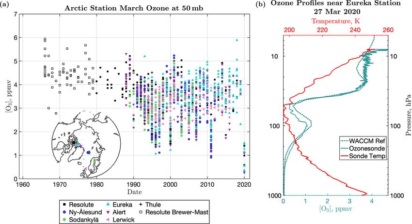
15772                                          C. Wilka et al.: An Arctic ozone hole in 2020 if not for the Montreal Protocol

the Ozone Layer, more commonly referred to as the Montreal          shown using both ozonesondes (Wohltmann et al., 2020) and
Protocol. The Montreal Protocol, and its subsequent amend-          satellites (Manney et al., 2020b). While the classical def-
ments during the 1990s, mandated the decrease and eventual          inition of an ozone hole (a significant areal extent below
cessation of the worldwide production of ozone-depleting            220 DU) did not occur in 2020, many news reports charac-
substances (ODSs) such as CFCs (Birmpili, 2018).                    terized it as such, sparking public uncertainty over whether
   Within the past few years, ever stronger evidence for            humanity has really solved the problem of ozone depletion.
global ozone stabilization and a nascent Antarctic ozone re-        Here we seek to examine the chemistry and ozone deple-
covery has emerged (Solomon et al., 2016; Sofieva et al.,           tion of both the RW and of that obtained in a world with-
2017; Chipperfield et al., 2017; Strahan and Douglass, 2018).       out the Montreal Protocol to evaluate what 2020 implies for
Despite uncertainties surrounding continuing CFC emissions          the Montreal Protocol’s achievements in the context of Arctic
from both scattered rogue production (Montzka et al., 2018)         ozone loss.
and existing stores in building foams and other banks (Lick-
ley et al., 2020), the world appears to be on track for near-
complete ozone recovery to near-1980s values as a result            2     Methods and data
of decreasing ODSs by the second half of the 21st century
(WMO, 2018), and the Montreal Protocol has been ratified            2.1    Model
by every state represented at the United Nations. No other
global environmental treaty can claim such a resounding suc-        We use the specified dynamics version of the National Cen-
cess.                                                               ter for Atmospheric Research’s (NCAR) Whole Atmosphere
   The success of the Montreal Protocol, however, should be         Community Climate Model (SD-WACCM) to compare the
measured not just by emission adherence but by the harm to          ozone depletion and chemistry in a simulation of the real
the Earth system and human society that its passage avoided.        world (RW) to one in which ODSs continued to increase by
The first study on such a “world avoided” (WA) by Prather           3.5 % per year from the year 1985 onwards (WA). The as-
et al. (1996) found strong evidence that the Antarctic ozone        sumption of a 3.5 % per year growth matches that used in
hole would have continued to worsen on average. Subse-              the Garcia et al. (2012) WA study and is a good approxi-
quent studies broadened to examine variability from year            mation of the growth rates seen in years immediately prior
to year and at various longitudes. A decade later, Morgen-          to emissions controls, thus representing an illustrative busi-
stern et al. (2008) studied WA in a more detailed three-            ness as usual alternate trajectory. The Community Earth Sys-
dimensional model and found significant ozone decline in            tem Model, version 2 (CESM2) WACCM is a superset of the
the upper stratosphere and polar vortices, a transition in the      Community Atmosphere Model, version 6 (CAM6), which
Arctic from dynamical to chemical control of ozone evolu-           extends from the Earth’s surface to the lower thermosphere
tion, and major regional climate impacts caused by dynami-          (Gettelman et al., 2019). WACCM includes updated repre-
cal changes. The first fully interactive time-evolving global       sentations of boundary layer processes, shallow convection
study of the world avoided by the Montreal Protocol, by             and liquid cloud macrophysics, and two-moment cloud mi-
Newman et al. (2009), found increasingly extreme impacts            crophysics with prognostic cloud mass and concentration
throughout the 21st century. Their simulations for the WA           (Danabasoglu et al., 2020). Aerosol representation for dust,
predicted Arctic column ozone levels of 220 DU or less by           sea salt black carbon, organic carbon, and sulfate in three size
2030, with some minimum values within the vortex that low           categories is prognostic in this version (Mills et al., 2016).
by 2020 in extremely cold years. The associated column de-          We use the specified dynamics (SDs) version of WACCM,
pletion was predicted to yield a 550 % increase in DNA dam-         where the atmosphere below 50 km is nudged to the Modern-
age when compared to 1980 by 2065 for Northern Hemi-                Era Retrospective Analysis for Research and Applications,
sphere (NH) midlatitudes. Chipperfield et al. (2015) exam-          version 2 (MERRA-2; Gelaro et al., 2017), temperature and
ined the WA for the recent extremely cold year of 2011. They        wind fields with a relaxation time of 50 h. There are 88
found that Arctic ozone levels would indeed have dropped            vertical pressure grid levels from the ground to the ther-
below 220 DU in that year in the WA but in a limited region         mosphere (∼ 140 km), with the altitude resolution increas-
that did not span the entire pole as in the Antarctic, as we        ing from ∼ 0.1 km near the surface to ∼ 1.0 km in the upper
discuss in Sect. 3. During a recent study quantifying drivers       troposphere–lower stratosphere (UTLS) and ∼ 1–2 km in the
of depletion in spring 2020 in the real world (RW; Feng et          stratosphere. The horizontal resolution is 1.95◦ × 2.5◦ in lat-
al., 2021), they updated their previous WA model and found          itude and longitude. All model results are taken from a 24 h
that the year 2020 would have seen much deeper column de-           average for each given day. The chemistry mechanism used
pletion during March than 2011 did (see their Supplement).          in this study includes a detailed representation of the mid-
   The Arctic spring of 2020 displayed very cold tempera-           dle atmosphere, with a sophisticated suite of gas-phase and
tures and a stable polar vortex that led to record levels of Arc-   heterogeneous chemistry reactions, including the Ox , NOx ,
tic PSCs and deep Arctic ozone depletion in the real world at       HOx , ClOx , and BrOx reaction families (Kinnison et al.,
some altitudes in the lower stratosphere, as has already been       2007). There are ∼ 100 chemical species and ∼ 300 chemical

Atmos. Chem. Phys., 21, 15771–15781, 2021                                           https://doi.org/10.5194/acp-21-15771-2021
C. Wilka et al.: An Arctic ozone hole in 2020 if not for the Montreal Protocol                                             15773

reactions. Reaction rates are updated following Jet Propul-       2.3    Ozonesondes
sion Laboratory (JPL) 2015 recommendations (Burkholder
et al., 2015). The model’s volcanic sulfur loading is from the    We use balloon-based ozonesondes to examine ozone mixing
Neely and Schmidt (2016) database and has been updated            ratios at individual levels and in vertical profiles. Ozoneson-
through the Raikoke eruption in 2019. Polar stratospheric         des are launched at regular intervals from multiple stations
clouds (PSCs) are present below ∼ 200 K as solid nitric acid      across the globe and are collated by the World Ozone and Ul-
trihydrate (NAT), water ice, and super-cooled ternary solu-       traviolet Data Centre. We use data from Resolute (74.86◦ N,
tions (Solomon et al., 2015). As described further in Sect. 3,    −94.98◦ E), Ny-Ålesund (78.93◦ N, 11.88◦ E), Sodankylä
to simulate ozone loss more accurately, we tested multiple        (67.34◦ N, 26.51◦ E), Eureka (80.04◦ N, −86.18◦ E), Alert
values of the parameterized NAT particle number density           (82.49◦ N, −62.42◦ E), Lerwick (60.13◦ N, −1.18◦ E), and
controlling denitrification in this model, ranging from the de-   Thule (76.53◦ N, −68.74◦ E) to represent the historical
fault of 0.01 to 10−5 particles per cubic centimeter, and chose   record of ozone mixing ratios at 50 mb. All data in recent
the smallest value for the final RW and WA simulations.           decades are from electrochemical concentration cell (ECC)
   The RW runs use the Coupled Model Intercomparison              ozonesondes, which have a precision of 3 %–5 % and an
Project phase 6 (CMIP6) hindcast scenario (Meinshausen et         overall uncertainty in ozone concentration of about ±10 %
al., 2017) based on observations for the evolution of ODSs        up to 30 km (Smit et al., 2007; Tarasick et al., 2021). The
and other emissions through 2014. The period from 2015            ozone sensor response time of ∼ 25 s, for a typical balloon
through April 2020 uses the CMIP6 Shared Socioeconomic            ascent rate of 4–5 m/s, gives ozonesondes a vertical resolu-
Pathways (SSPs) 585 projection (O’Neill et al., 2016). The        tion of about 100–150 m. Pre-1980 data from Resolute are
WA run assumes a 3.5 % per year increase, beginning in            from older Brewer–Mast sondes, which have a precision of
1985, in all organic chlorine and bromine species, except         about 5 %–10 % (Kerr et al., 1994; Smit and Kley, 1998).
for CH3 Cl, CH2 Br2 , and CHBr3 , which mainly have natu-         For profile comparisons, we use ECC ozonesondings from
ral sources (Fig. S1 in the Supplement). CH3 Br is assumed        Eureka, Alert, and Resolute, along with simultaneously mea-
to be half from natural sources and half from anthropogenic,      sured temperatures.
so its increase is half that of the other ODSs.

2.2   Satellites                                                  3     Results
We compare SD-WACCM’s total column ozone values to                Figure 1 shows the total column ozone (TCO) that would
those observed by NASA’s Ozone Monitoring Instrument              have been expected in the WA (top left) on the day of the
(OMI) on the Earth Observing System (EOS) Aura satellite          greatest ozone depletion in 2020 in the model, 13 March,
(Bhartia, 2012). OMI is a nadir-viewing wide-field-imaging        compared to that expected and observed in the RW run (top
spectrometer that continues the global total column ozone         right; bottom right) for the same day. The area meeting the
record from NASA’s Total Ozone Mapping Spectrometer               standard definition of an ozone hole in the WA is nearly
(TOMS). We use the Level 3 gridded data product here for          20 million km2 , which is a comparable areal extent to many
comparison with SD-WACCM’s daily column ozone values.             observed past Antarctic ozone holes, and the region below
Level 3 data is generated from high-quality Level 2 data and      150 DU stretches across the North Pole and over signifi-
is available on a daily basis. When calculating the daily polar   cant parts of Canada, Greenland, and Russia. By comparison,
cap minimum total ozone values, we filter the data at solar       while the depletion in the RW case is clearly visible, it never
zenith angles above 82◦ to remove spurious points.                breaches the 220 DU threshold for any significant area. Ob-
   We compare SD-WACCM’s HNO3 mixing ratios to those              servations from OMI (lower right) support this, although the
observed by NASA’s Microwave Limb Sounder (MLS) on                higher-resolution satellite finds small, isolated patches below
the EOS Aura satellite (Waters et al., 2006; Lambert et al.,      220 DU. The difference between the WA and RW runs (lower
2007). MLS has been continuously observing the upper at-          left) is 20 DU or more throughout the Northern Hemisphere
mosphere since its launch in 2004, although data gaps ex-         and maximizes at over 130 DU in the Arctic. We can com-
ist, including during the second half of March through early      pare this to another recent cold year, i.e, 2011 (Fig. S2), pre-
April 2020. MLS data were processed according to the flags        viously highlighted by others for its large Arctic ozone losses
and thresholds described in the Version 4.2× Level 2 Data         in a WA simulation (Chipperfield et al., 2015; compare our
Quality and Description document. The vertical resolution         Fig. S2 with their Fig. 3). We note that our study follows a
of the HNO3 data at the levels of interest is 3–4 km, with a      slightly different WA emissions path, with a different par-
reported measurement precision of ±0.6 ppbv (parts per bil-       titioning between anthropogenic and natural emissions for
lion by volume) and a systematic uncertainty of ±1.0 ppbv.        CH3 Br in particular (Chipperfield et al., 2015; compare our
MLS data were binned into a 5◦ × 5◦ latitude–longitude grid       Fig. S1 with their Fig. 1a). In our simulations, the expected
before plotting.                                                  Arctic ozone hole in 2011 is much smaller in area than in
                                                                  2020 (11.08 million km2 vs. 19.71 million km2 ). The differ-

https://doi.org/10.5194/acp-21-15771-2021                                         Atmos. Chem. Phys., 21, 15771–15781, 2021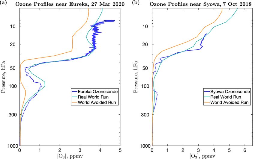
15774 C. Wilka et al.: An Arctic ozone hole in 2020 if not for the Montreal Protocol
ence is partly due to the increased chlorine loading in the
WA 9 years later, but we also note that, while 2011 was an
extremely cold year, 2020 had lower minimum ozone values
that lasted longer than in 2011, with record fractions of the
polar vortex being below the PSC temperature threshold for
a longer period of time (Wohltmann et al., 2020; Inness et
al., 2020). In summary, without the Montreal Protocol, the
2020’s combination of extreme meteorology and increased
chlorine loading would have resulted in unprecedented Arc-
tic ozone depletion and an Arctic ozone hole comparable in
areal extent to those of the Antarctic, with accompanying
large impacts on UV levels throughout the Arctic.
To confirm the historically anomalous nature of 2020 and
to evaluate our model’s performance in more detail, we ex-
amine a time series of measurements at the 50 mb pressure
level from archived Arctic ozonesondes (left panel of Fig. 2).
Because 2020 displayed very large local changes in Arctic
ozone, the less-precise measurements from older Brewer–
Mast sondes are also valuable for this purpose and are shown
with open symbols. The long ozonesonde record allows us to
compare to historical values predating the start of the satellite
Figure 1. Total column ozone poleward of 30◦ N for
era in 1979, which is especially important for ozone trends
13 March 2020. Panel (a) shows the WA SD-WACCM run,
as there may have been some depletion already by that time. panel(b) shows the RW run, and panel (c) shows the difference
Figure 2 shows ozone values for available days in March, between them. Panel (d) shows the total column ozone Level 3
stacked by year, and demonstrates that 2020 displays ozone product from the OMI satellite. All levels are in Dobson units. Note
amounts lower than any other year in the record at this alti- the different scale in the lower left color bar. The 220 DU contour
tude (including 2011, which displays the next deepest deple- is outlined in white.
tion). This is especially apparent in the log-scale version in
Fig. S3.
The right panel of Fig. 2 compares the vertical profile of and ozonesonde profiles. Polar stratospheric clouds not only
ozone at the nearest SD-WACCM grid point in the RW sim- activate chlorine through heterogeneous chemical process-
ulation (dotted teal line) to Eureka Station ozonesonde data ing but also denitrify the atmosphere through removal of
(solid teal line) for 27 March 2020, showing some of the low- HNO3 from the gas phase and subsequent sedimentation.
est values of stratospheric ozone ever recorded in the Arctic. Removing HNO3 reduces the abundance of NO2 , which,
Eureka is near the center of the lowest total ozone on this in turn, enhances active chlorine (i.e., ClO abundances) by
date and is representative of the region based upon the model, reducing ClONO2 formation rates, affecting ozone destruc-
and on comparisons with other high-Arctic sites, which show tion chemistry. Initial comparisons of ozone profiles to both
similar profiles. The figure shows that the largest depletion ozonesonde and MLS data showed that the model’s standard
here tracks the lowest local temperatures of the profile (tem- approach with a NAT density of 0.01 cm−3 (Wegner et al.,
perature shown in solid red). Although temperature histo- 2013) was denitrifying too little. As a lower NAT particle
ries can also be important, as activation can persist in air density corresponds to larger individual particles, decreasing
parcels which previously encountered cold air but are cur- this parameter increases denitrification by increasing the set-
rently above the temperature threshold for PSC formation; tling velocity of the particles. Figure 3a–d show the progres-
this broadly supports the view that much of this year’s ozone sion of four increasingly denitrified RW runs.
loss was related to widespread local cold temperatures in- Although the coverage of MLS data swaths (Fig. 3e)
creasing the efficiency of heterogeneous reactions on PSCs makes it difficult to distinguish which of the two highest
(Wohltmann et al., 2020; Manney et al., 2020b). Figure 2 il- (Fig. 3c and d) denitrification levels might be a better rep-
lustrates that the SD-WACCM model successfully captures resentation, the two lower denitrification levels (Fig. 3a and
the observed behavior at this site under these extreme condi- b) are much poorer matches to the observations. We ulti-
tions. mately found that a case adopting a NAT particle density
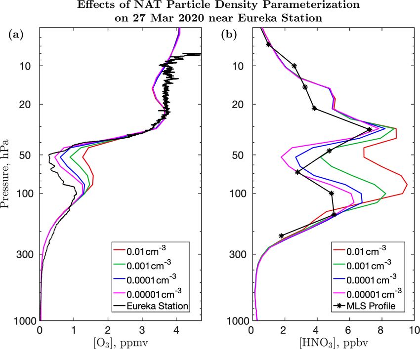
We next test how SD-WACCM’s nitric acid trihydrate of 10−5 particles per cubic centimeter resulted in the closest
(NAT) number density count relates to calculated denitrifi- match to observed ozone profiles throughout a wide vertical
cation (Fahey et al., 2001), using comparisons to nitric acid range throughout the spring (Fig. 4a for Eureka on 27 March;
observations from the Microwave Limb Sounder (MLS) in- Fig. S4 for other times at Eureka, along with the Alert and
strument onboard the Aura satellite (Waters et al., 2006) Resolute stations) and matched the observed MLS HNO3
Atmos. Chem. Phys., 21, 15771–15781, 2021 https://doi.org/10.5194/acp-21-15771-2021C. Wilka et al.: An Arctic ozone hole in 2020 if not for the Montreal Protocol 15775 Figure 2. (a) Daily ozone values centered at 50 mb (±2.5 mb) from ozonesondes launched from various stations across the northern polar region in March. Measurements using less accurate methods are indicated with open symbols. The location of these stations is shown in the lower left corner of the panel. (b) Ozone (solid teal) and temperature (solid red) profiles taken at Eureka Station on 27 March 2020, compared to the SD-WACCM RW run’s (dotted teal) vertical profile at the nearest model grid point. Figure 3. HNO3 in parts per billion by volume, for 20 February 2020, for different NAT parameterizations in SD-WACCM (a–d) compared to MLS (e). In order of increasing denitrification, the NAT density is (a) 0.01 cm−3 , (b) 0.001 cm−3 , (c) 0.0001 cm−3 , and (d) 0.00001 cm−3 . Panel (a) shows the previous standard SD-WACCM parameterization, and panel (d) shows the chosen parameter value used in the RW and WA simulations. All SD-WACCM figures show the 73 mb level; MLS (e) shows the 68 mb level. https://doi.org/10.5194/acp-21-15771-2021 Atmos. Chem. Phys., 21, 15771–15781, 2021
15776 C. Wilka et al.: An Arctic ozone hole in 2020 if not for the Montreal Protocol
accurate representation of denitrification (not only accurate
temperature-driven reaction efficiencies but also PSC micro-
physics impacts) is key for ozone depletion under 2020 Arc-
tic conditions.
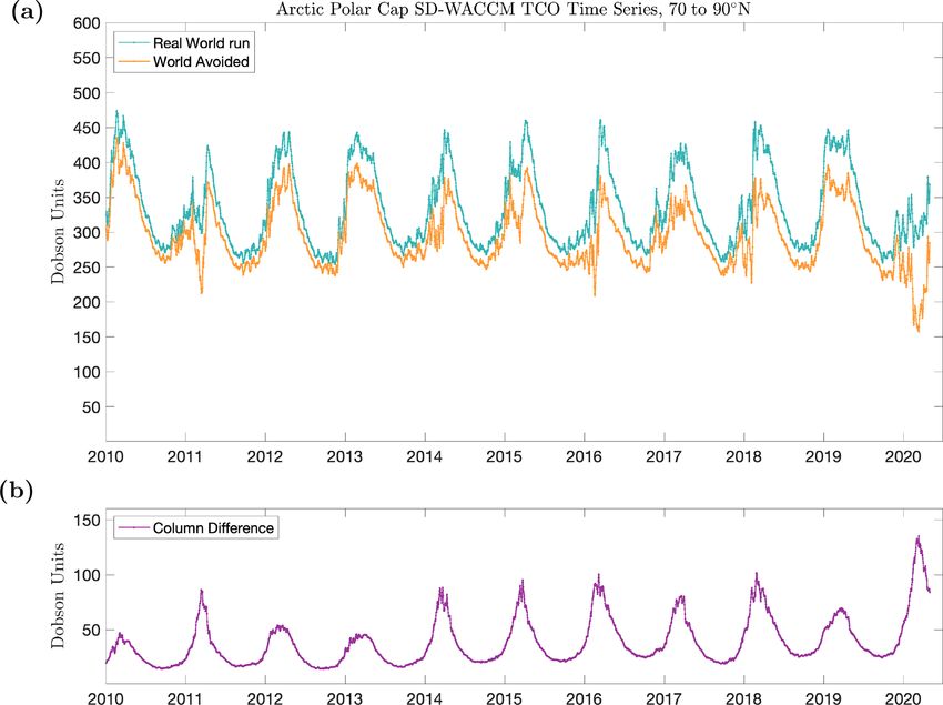
In Fig. 5, we examine the evolution of daily minimum
TCO by day of the year from January 2010 to the end of
April 2020 for the polar cap north of 70◦ N, with days in
2020 marked with open circles rather than points. We com-
pare the RW (teal markers) to observations from the OMI
satellite (blue markers) and compare both with the WA (or-
ange markers). Dramatic differences are obtained in the cal-
culated and observed 2020 evolution of the daily minimum
TCO value over the Arctic polar cap by day of the year for the
past decade in Fig. 5 compared to the preceding years and es-
pecially for the WA. Prior to 2020, while the WA case is often
lower than the other two, it is still within the range of TCO
values seen in the RW and OMI time series. Furthermore,
both the RW run and the OMI observations for 2020 spring
Figure 4. Comparison of ozone profiles (a) and nitric acid profiles display lower values than many WA springs, illustrating the
(b) for four different SD-WACCM simulations at the grid point key role of the unusually cold temperatures in addition to
nearest Eureka Station for 27 March 2020, with ozonesonde data
chlorine in driving the depletion in 2020. The WA spring of
from Eureka Station shown for comparison in (a) and the nearest
MLS profile on that day shown for comparison in (b). Note that
2020 displays levels of depletion previously unseen in the
MLS has very few levels in the lower stratosphere (shown by black data or either simulation early in the spring and stays de-
points). This is the same date as shown in Fig. 2b, and the magenta pleted longer than any other year. Furthermore, its apparent
ozone profile corresponds to the dotted teal ozone profile shown in dip compared to the rest of the year resembles typical Antarc-
that figure. tic ozone evolution (shown in Fig. S5) rather than the typical
Arctic behavior. The effects of higher chlorine loading in the
WA scenario on vertical ozone profiles are also significant
(Fig. 6; left panel). While both the RW run and ozonesonde
data display a limited height region of extremely low ozone,
the WA has almost no ozone left throughout the lower strato-
sphere. This resembles typical Antarctic depletion more than
any previous year in the Arctic (Fig. 6; right panel; with
ozonesonde comparison). Depletion in the lower stratosphere
reaches these low values more quickly in the WA and persists
longer (Fig. S6). At higher altitudes, where the gas-phase de-
pletion identified by Molina and Rowland (1974) is domi-
nant, substantial increases in depletion are also obtained (see
below).
A characteristic finding of WA studies is that substantial
polar ozone depletion eventually persists year-round (New-
man et al., 2009; Garcia et al., 2012). We can see the first
indication of such behavior in our WA simulation for 2020,
as shown in Fig. 7, where the RW and WA total ozone time
Figure 5. Minimum total column ozone simulated by SD-WACCM
from 70 to 90◦ N from January 2010 through the end of April 2020, series are shown for the past decade (top panel), along with
plotted by day of the year. Teal markers refer to the reference run their difference (bottom panel). While for the first few years
and orange markers to the WA run. Blue markers refer to observa- of the decade the summertime and autumnal differences be-
tions by the OMI satellite. Dots indicate days from 2010 to 2019, tween the scenarios remain low and fairly constant, after
and open circles indicate days in 2020. 2014 a noticeable trend towards increasing column differ-
ence year-round emerges. Much of this summertime differ-
ence is due to the gas-phase depletion, as demonstrated by
profiles better than other choices (Fig. 4b), and so chose this the change in the profiles and increased partial column dif-
value for our RW and WA simulations. As all of our RW ferences at higher altitudes (Fig. S7). It is also noteworthy
runs adopt observed temperatures insofar as they are repre- that, while the spring of 2020 is anomalously depleted in the
sented by the MERRA-2 reanalysis, this study illustrates that WA as previously shown, the spring ozone values obtained
Atmos. Chem. Phys., 21, 15771–15781, 2021 https://doi.org/10.5194/acp-21-15771-2021C. Wilka et al.: An Arctic ozone hole in 2020 if not for the Montreal Protocol 15777 Figure 6. Comparison between the RW (teal) and WA (orange) ozone profiles in SD-WACCM at the grid point (a) nearest to Eureka Station (80.04◦ N, −86.18◦ E) for 27 March 2020 and (b) nearest to Syowa Station in the Antarctic (69.00◦ S, 39.58◦ E) for 7 October 2018. Ozonesonde profiles from the stations are shown, for comparison, in blue. Figure 7. (a) Time series of mean SD-WACCM total column ozone across the polar cap for the RW scenario (teal) and WA scenario (orange) from January 2010 through April 2020. (b) The difference between the two. https://doi.org/10.5194/acp-21-15771-2021 Atmos. Chem. Phys., 21, 15771–15781, 2021
15778                                          C. Wilka et al.: An Arctic ozone hole in 2020 if not for the Montreal Protocol

Table 1. Surface UV index for the SD-WACCM grid point nearest to Fairbanks, USA (64.84◦ N, 147.7◦ W), Yellowknife, Canada (62.46◦ N,
114.22◦ W), Tromsø, Norway (69.66◦ N, 18.94◦ E), and Murmansk, Russia (68.96◦ N, 33.08◦ E). The UV index is calculated for 31 March
and 30 April for both the RW and WA simulations, using total column ozone and solar zenith angle at noon under clear-sky conditions in
each grid point.

                                           RW March 31      WA March 31      RW April 30     WA April 30
                            Fairbanks                1.15            1.44            2.49            3.06
                            Yellowknife              1.62            2.52            3.05            3.75
                            Tromsø                   1.12            1.93            2.32            2.75
                            Murmansk                 1.27            2.39            2.19            2.66

in 2018 and 2019 are also much further from their RW coun-           nearest four northern cities using the procedure outlined in
terparts, demonstrating the growing impact of the Montreal           Burrows et al. (1994), with the results shown in Table 1.
Protocol even for less cold years.                                   While the UV indices at the end of March in the WA run
                                                                     show substantial percentage increases (from 25 % to 88 %),
                                                                     the absolute values are still quite small due to the large zenith
4   Discussion and conclusions                                       angles in the Arctic spring. By the end of April, however,
                                                                     there are still substantial differences between the runs, de-
We have demonstrated that, were it not for the Montreal Pro-         spite active ozone depletion having ceased for the year, rein-
tocol, the meteorological conditions seen in 2020 would have         forcing that there are increasing year-round impacts, as seen
produced the first Antarctic-like ozone hole over the Arc-           in Fig. 7.
tic, an area with a substantial human population and vibrant            The benefits to society and the Earth system achieved by
ecosystem. The Arctic ozone hole would have begun earlier            the global community’s adherence to the Montreal Protocol
and persisted longer (see Fig. S6) than the headline-grabbing        grow with each passing year and can be dramatically docu-
2020 ozone depletion in the real world did, with ozone all but       mented in cold years with ozone-depletion-favoring meteo-
completely destroyed over a large vertical extent of the lower       rology – in particular, 2020. As we progress further into the
stratosphere. Furthermore, our simulations support the view          21st century, studies of the world we avoided will continue to
that there have already been substantial year-round benefits         be relevant to both stratospheric science and environmental
from the Montreal Protocol for the Arctic. Finally, nitric acid      policy. When the Montreal Protocol was signed, the sophisti-
observations and modeling for 2020 help improve our under-           cated modeling systems used for this and similar studies that
standing of the role of denitrification in accurately assessing      can precisely simulate an alternate world did not yet exist.
Arctic ozone loss, and further refinements of this will be the       The basic science was, however, sound enough, and the risk
subject of future studies.                                           clear enough, that society acted nonetheless. Here we have
   The main limitation of using a model constrained to real-         shown that our increased knowledge of what we would have
world meteorology is that it, by design, eliminates any feed-        faced has justified this past prudence.
backs that changes in ozone would have had on the mete-
orology. These are worthy of investigation in future free-
running model simulations, especially in the context of po-          Data availability. MERRA-2, OMI, and MLS data can all
tential increasing stratospheric Arctic cold extremes from cli-      be freely obtained online from NASA (https://gmao.gsfc.
mate change, which have been debated in the literature (Rex          nasa.gov/reanalysis/MERRA-2/data_access, last access: 19
et al., 2004). In addition to the increased radiative forcing        October 2021; https://doi.org/10.5067/Aura/OMI/DATA3002,
from increasing ODSs, ozone itself is a potent local green-          Bhartia, 2012; https://doi.org/10.5067/Aura/MLS/DATA2511,
house gas, and ozone depletion of the magnitude simulated            Manney et al., 2020a). Ozonezonde station data can be
                                                                     accessed through the World Ozone and Ultraviolet Data
here would significantly alter the temperature profile in the
                                                                     Center        (WOUDC;          https://doi.org/10.14287/10000001,
stratosphere and perhaps in the troposphere as well. Resul-          WMO/GAW Ozone Monitoring Community et al., 2021).
tant changes in stratospheric dynamics could potentially have        Model results shown in this paper are available online
then led to changes in surface climate and sea ice (Smith et         (https://acomstaff.acom.ucar.edu/dkin/ACP_Wilka_2020/,        last
al., 2018; Stone et al., 2019, 2020). Surface UV increases           access: 29 October 2020).
could be especially important during the Arctic summer,
when the vast majority of biological growth takes place. A
coupled biosphere model would be required to fully inves-            Supplement. The supplement related to this article is available on-
tigate such effects, but we can estimate the change in sur-          line at: https://doi.org/10.5194/acp-21-15771-2021-supplement.
face UV during late March and April 2020 by calculating the
clear-sky UV index at noon for the SD-WACCM grid point

Atmos. Chem. Phys., 21, 15771–15781, 2021                                             https://doi.org/10.5194/acp-21-15771-2021
C. Wilka et al.: An Arctic ozone hole in 2020 if not for the Montreal Protocol 15779
Author contributions. DK, SS, and CW contributed to the model- ber, M.: Detecting recovery of the stratospheric ozone layer, Na-
ing run setup and interpretation. DT contributed to data interpreta- ture, 549, 211–218, 2017.
tion. All authors contributed to writing the paper. Crutzen, P. J. and Arnold, F.: Nitric acid cloud formation in the cold
Antarctic stratosphere: A major cause for the springtime “ozone
hole”, Nature, 324, 651–655, 1986.
Competing interests. The authors declare that they have no conflict Danabasoglu, G., Lamarque, J. F., Bacmeister, J., Bailey, D. A.,
of interest. DuVivier, A. K., Edwards, J., Emmons, L. K., Fasullo, J., Gar-
cia, R., Gettelman, A., and Hannay, C.: The Community Earth
System Model version 2 (CESM2), J. Adv. Model Earth Syst.,
Disclaimer. Publisher’s note: Copernicus Publications remains 12, e2019MS001916, https://doi.org/10.1029/2019MS001916,
neutral with regard to jurisdictional claims in published maps and 2020.
institutional affiliations. Fahey, D. W., Gao, R. S., Carslaw, K. S., Kettleborough, J., Popp,
P. J., Northway, M. J., Holecek, J. C., Ciciora, S. C., McLaugh-
lin, R. J., Thompson, T. L., and Winkler, R. H.: The detection
of large HNO3 -containing particles in the winter Arctic strato-
Acknowledgements. WACCM is a component of the CESM, sup-
sphere, Science, 291, 1026–1031, 2001.
ported by the National Science Foundation (NSF). We would like to
Farman, J. C., Gardiner, B. G., and Shanklin, J. D.: Large losses of
acknowledge high-performance computing support from Cheyenne
total ozone in Antarctica reveal seasonal ClOx /NOx interaction,
(https://doi.org/10.5065/D6RX99HX) provided by NCAR’s Com-
Nature, 315, 207–210, 1985.
putational and Information Systems Laboratory and sponsored by
Feng, W., Dhomse, S. S., Arosio, C., Weber, M., Burrows, J.
the NSF.
P., Santee, M. L., and Chipperfield, M. P.: Arctic ozone de-
pletion in 2019/20: Roles of chemistry, dynamics and the
Montreal Protocol, Geophys. Res. Lett., 48, e2020GL091911,
Financial support. Catherine Wilka and Susan Solomon were https://doi.org/10.1029/2020GL091911, 2021.
partly supported by a gift from an anonymous donor to Garcia, R. R., Kinnison, D. E., and Marsh, D. R.: “World
MIT. Doug Kinnison was funded in part by NASA (grant avoided” simulations with the whole atmosphere commu-
no. 80NSSC19K0952). nity climate model, J. Geophys. Res.-Atmos., 117, D23303,
https://doi.org/10.1029/2012JD018430, 2012.
Gelaro, R., McCarty, W., Suárez, M. J., Todling, R., Molod, A.,
Review statement. This paper was edited by Yafang Cheng and re- Takacs, L., Randles, C. A., Darmenov, A., Bosilovich, M. G., Re-
viewed by two anonymous referees. ichle, R., and Wargan, K.: The modern-era retrospective analysis
for research and applications, version 2 (MERRA-2), J. Climate,
30, 5419–5454, 2017.
Gettelman, A., Mills, M. J., Kinnison, D. E., Garcia, R. R., Smith,
References A. K., Marsh, D. R., Tilmes, S., Vitt, F., Bardeen, C. G., McIn-
erny, J., and Liu, H. L.: The whole atmosphere community cli-
Bhartia, P. K.: Data from “OMI/Aura TOMS-Like ozone and ra- mate model version 6 (WACCM6), J. Geophys. Res.-Atmos.,
diative cloud fraction L3 1 day 0.25 degree x 0.25 degree V3”, 124, 12380–12403, 2019.
NASA Goddard Space Flight Center, Goddard Earth Sciences Hofmann, D. J., Oltmans, S. J., Harris, J. M., Johnson, B. J., and
Data and Information Services Center (GES DISC) [date set], Lathrop, J. A.: Ten years of ozonesonde measurements at the
https://doi.org/10.5067/Aura/OMI/DATA3002, 2012. south pole: Implications for recovery of springtime Antarctic
Birmpili, T.: Montreal Protocol at 30: The governance structure, ozone, J. Geophys. Res.-Atmos., 102, 8931–8943, 1997.
the evolution, and the Kigali Amendment, Collect C. R. Geosci., Inness, A., Chabrillat, S., Flemming, J., Huijnen, V., Langen-
350, 425–431, 2018. rock, B., Nicolas, J., Polichtchouk, I., and Razinger, M.: Ex-
Burkholder, J. B., Sander, S. P., Abbatt, J. P. D., Barker, J. R., Huie, ceptionally low Arctic stratospheric ozone in spring 2020 as
R. E., Kolb, C. E., Kurylo, M. J., Orkin, V. L., Wilmouth, D. seen in the CAMS reanalysis, J. Geophys. Res.-Atmos., 125,
M., and Wine, P. H.: Chemical kinetics and photochemical data e2020JD033563, https://doi.org/10.1029/2020JD033563, 2020.
for use in atmospheric studies: Evaluation number 18, Techni- Kerr, J. B., Fast, H., McElroy, C. T., Oltmans, S. J., Lathrop, J. A.,
cal Report, Pasadena, CA: Jet Propulsion Laboratory, National Kyro, E., Paukkunen, A., Claude, H., Köhler, U., Sreedharan, C.
Aeronautics and Space Administration, 2015. R., and Takao, T.: The 1991 WMO international ozonesonde in-
Burrows, W. R., Vallée, M., Wardle, D. I., Kerr, J. B., Wilson, L. tercomparison at Vanscoy, Canada, Atmosphere-Ocean, 32, 685–
J., and Tarasick, D. W.: The Canadian operational procedure for 716, 1994.
forecasting total ozone and UV radiation, Meteorol. Appl., 1, Kinnison, D. E., Brasseur, G. P., Walters, S., Garcia, R. R.,
247–265, 1994. Marsh, D. R., Sassi, F., Harvey, V. L., Randall, C. E., Em-
Chipperfield, M. P., Dhomse, S. S., Feng, W., McKenzie, R. L., mons, L., Lamarque, J. F., and Hess, P.: Sensitivity of chem-
Velders, G. J., and Pyle, J. A.: Quantifying the ozone and ultra- ical tracers to meteorological parameters in the MOZART-
violet benefits already achieved by the Montreal Protocol, Nat. 3 chemical transport model, J. Geophys. Res., 112, D20302,
Commun., 6, 1–8, 2015. https://doi.org/10.1029/2006JD007879, 2007.
Chipperfield, M. P., Bekki, S., Dhomse, S., Harris, N. R., Has-
sler, B., Hossaini, R., Steinbrecht, W., Thiéblemont, R., and We-
https://doi.org/10.5194/acp-21-15771-2021 Atmos. Chem. Phys., 21, 15771–15781, 202115780 C. Wilka et al.: An Arctic ozone hole in 2020 if not for the Montreal Protocol Lambert, A., Read, W. G., Livesey, N. J., Santee, M. L., Manney, Newman, P. A., Oman, L. D., Douglass, A. R., Fleming, E. L., Frith, G. L., Froidevaux, L., Wu, D. L., Schwartz, M. J., Pumphrey, S. M., Hurwitz, M. M., Kawa, S. R., Jackman, C. H., Krotkov, N. H. C., Jimenez, C., and Nedoluha, G. E.: Validation of the Aura A., Nash, E. R., Nielsen, J. E., Pawson, S., Stolarski, R. S., and Microwave Limb Sounder middle atmosphere water vapor and Velders, G. J. M.: What would have happened to the ozone layer nitrous oxide measurements, J. Geophys. Res., 112, D24S36, if chlorofluorocarbons (CFCs) had not been regulated?, Atmos. https://doi.org/10.1029/2007JD008724, 2007. Chem. Phys., 9, 2113–2128, https://doi.org/10.5194/acp-9-2113- Langematz, U., Tully, M., Calvo, N., Dameris, M., Laat, J. de., 2009, 2009. Klekociuk, A., Müller, R., and Young, P.: Polar stratospheric O’Neill, B. C., Tebaldi, C., van Vuuren, D. P., Eyring, V., Friedling- ozone: past, present, and future, chap. 4, in: Scientific Assess- stein, P., Hurtt, G., Knutti, R., Kriegler, E., Lamarque, J.-F., ment of Ozone Depletion: 2018, Global Ozone Research and Lowe, J., Meehl, G. A., Moss, R., Riahi, K., and Sander- Monitoring Project-Report No. 58, World Meteorological Orga- son, B. M.: The Scenario Model Intercomparison Project (Sce- nization, Geneva, Switzerland, 20, 2018. narioMIP) for CMIP6, Geosci. Model Dev., 9, 3461–3482, Lickley, M., Solomon, S., Fletcher, S., Velders, G. J., Daniel, J., https://doi.org/10.5194/gmd-9-3461-2016, 2016. Rigby, M., Montzka, S. A., Kuijpers, L. J., and Stone, K.: Quan- Prather, M., Midgley, P., Rowland, F. S., and Stolarski, R.: The tifying contributions of chlorofluorocarbon banks to emissions ozone layer: the road not taken, Nature, 381, 551–554, 1996. and impacts on the ozone layer and climate, Nat. Commun., 11, Rex, M., Salawitch, R. J., von der Gathen, P., Harris, N. 1–11, 2020. R. P., Chipperfield, M. P., and Naujokat, B.: Arctic ozone Manney, G., Santee, M., Froidevaux, L., Livesey, N., and Read, loss and climate change, Geophys. Res. Lett., 31, L04116, W.: MLS/Aura Level 2 Nitric Acid (HNO3) Mixing Ratio https://doi.org/:10.1029/2003GL018844, 2004. V005, Greenbelt, MD, USA, Goddard Earth Sciences Data Smit, H. G. and Kley, D.: JOSIE: the 1996 WMO international in- and Information Services Center (GES DISC) [data set], tercomparison of ozonesondes under quasi-flight conditions in https://doi.org/10.5067/Aura/MLS/DATA2511, 2020a. the environmental chamber at Jülich, Proceedings of the XVIII Manney, G. L., Livesey, N. J., Santee, M. L., Froidevaux, L., Quadrennial Ozone Symposium, 971–974, 1998. Lambert, A., Lawrence, Z. D., Millán, L. F., Neu, J. L., Smit, H. G., Straeter, W., Johnson, B. J., Oltmans, S. J., Davies, Read, W. G., Schwartz, M. J. and Fuller, R. A.: Record- J., Tarasick, D. W., Hoegger, B., Stubi, R., Schmidlin, F. J., low Arctic stratospheric ozone in 2020: MLS observations Northam, T., and Thompson, A. M.: Assessment of the per- of chemical processes and comparisons with previous ex- formance of ECC-ozonesondes under quasi-flight conditions in treme winters, Geophys. Res. Lett., 47, e2020GL089063, the environmental simulation chamber: Insights from the Juelich https://doi.org/10.1029/2020JD033563, 2020b. Ozone Sonde Intercomparison Experiment (JOSIE), J. Geophys. Meinshausen, M., Vogel, E., Nauels, A., Lorbacher, K., Mein- Res., 112, 563–518, 2007. shausen, N., Etheridge, D. M., Fraser, P. J., Montzka, S. A., Smith, K. L., Polvani, L. M., and Tremblay, L. B.: The impact of Rayner, P. J., Trudinger, C. M., Krummel, P. B., Beyerle, U., stratospheric circulation extremes on minimum Arctic sea ice ex- Canadell, J. G., Daniel, J. S., Enting, I. G., Law, R. M., Lun- tent, J. Climate, 31, 7169–7183, 2018. der, C. R., O’Doherty, S., Prinn, R. G., Reimann, S., Rubino, Sofieva, V. F., Kyrölä, E., Laine, M., Tamminen, J., Degenstein, D., M., Velders, G. J. M., Vollmer, M. K., Wang, R. H. J., and Bourassa, A., Roth, C., Zawada, D., Weber, M., Rozanov, A., Weiss, R.: Historical greenhouse gas concentrations for cli- Rahpoe, N., Stiller, G., Laeng, A., von Clarmann, T., Walker, mate modelling (CMIP6), Geosci. Model Dev., 10, 2057–2116, K. A., Sheese, P., Hubert, D., van Roozendael, M., Zehner, C., https://doi.org/10.5194/gmd-10-2057-2017, 2017. Damadeo, R., Zawodny, J., Kramarova, N., and Bhartia, P. K.: Mills, M. J., Schmidt, A., Easter, R., Solomon, S., Kinnison, D. E., Merged SAGE II, Ozone_cci and OMPS ozone profile dataset Ghan, S. J., Neely III, R. R., Marsh, D. R., Conley, A., Bardeen, and evaluation of ozone trends in the stratosphere, Atmos. Chem. C. G., and Gettelman, A.: Global volcanic aerosol properties de- Phys., 17, 12533–12552, https://doi.org/10.5194/acp-17-12533- rived from emissions, 1990–2014, using CESM1(WACCM), J. 2017, 2017. Geophys. Res.-Atmos., 121, 2332–2348, 2016. Solomon, S., Garcia, R. R., Rowland, F. S., and Wuebbles, D. J.: On Molina, M. J. and Rowland, F. S.: Stratospheric sink for chloroflu- the depletion of Antarctic ozone, Nature, 321, 755–758, 1986. oromethanes: chlorine atom-catalysed destruction of ozone, Na- Solomon, S., Kinnison, D. E., Bandoro, J., and Garcia, R. R.: Sim- ture, 249, 810–812, 1974. ulation of polar ozone depletion: An update, J. Geophys. Res.- Montzka, S. A., Dutton, G. S., Yu, P., Ray, E., Portmann, R. W., Atmos., 120, 7958–7974, 2015. Daniel, J. S., Kuijpers, L., Hall, B. D., Mondeel, D., Siso, C., Solomon, S., Ivy, D. J., Kinnison, D., Mills, M. J., Neely, R. R., and and Nance, J. D.: An unexpected and persistent increase in global Schmidt, A.: Emergence of healing in the Antarctic ozone layer, emissions of ozone-depleting CFC-11, Nature, 557, 413–417, Science, 353, 269–274, 2016. 2018. Stolarski, R. S., Schoeberl, M. R., Newman, P. A., McPeters, R. D., Morgenstern, O., Braesicke, P., Hurwitz, M. M., O’Connor, F. M., and Krueger, A. J.: The 1989 Antarctic ozone hole as observed Bushell, A. C., Johnson, C. E., and Pyle, J. A.: The world avoided by TOMS, Geophys. Res. Lett., 17, 1267–1270, 1990. by the Montreal Protocol, Geophys. Res. Lett., 35, L16811, Stone, K. A., Solomon, S., and Kinnison, D. E.: Prediction of North- https://doi.org/10.1029/2008GL034590, 2008. ern Hemisphere regional sea ice extent and snow depth using Neely, R. R. and Schmidt, A.: VolcanEESM: Global volcanic sul- stratospheric ozone information, J. Geophys. Res.-Atmos., 125, phur dioxide (SO2 ) emissions database from 1850 to present – e2019JD031770, https://doi.org/10.1029/2019JD031770, 2020. Version 1.0, https://doi.org/10.5285/76ebdc0b-0eed-4f70-b89e- Stone, K. A., Solomon, S., Kinnison, D. E., Baggett, C. F., and 55e606bcd568, 2016. Barnes, E. A.: Prediction of Northern Hemisphere regional sur- Atmos. Chem. Phys., 21, 15771–15781, 2021 https://doi.org/10.5194/acp-21-15771-2021
C. Wilka et al.: An Arctic ozone hole in 2020 if not for the Montreal Protocol                                                     15781

   face temperatures using stratospheric ozone information, J. Geo-      Wegner, T., Kinnison, D. E., Garcia, R. R., and Solomon, S.: Sim-
   phys. Res.-Atmos., 124, 5922–5933, 2019.                                ulation of polar stratospheric clouds in the specified dynamics
Strahan, S. E. and Douglass, A. R.: Decline in Antarctic ozone de-         version of the whole atmosphere community climate model, J.
   pletion and lower stratospheric chlorine determined from Aura           Geophys. Res.-Atmos., 118, 4991–5002, 2013.
   Microwave Limb Sounder observations, Geophys. Res. Lett., 45,         Wohltmann, I., von der Gathen, P., Lehmann, R., Maturilli, M.,
   382–390, 2018.                                                          Deckelmann, H., Manney, G. L., Davies, J., Tarasick, D.,
Tarasick, D. W., Smit, H. G. J., Thompson, A. M., Mor-                     Jepsen, N., Kivi, R., and Lyall, N.: Near-complete local re-
   ris, G. A., Witte, J. C., Davies, J., Nakano, T., van                   duction of Arctic stratospheric ozone by severe chemical loss
   Malderen, R., Stauffer, R. M., Deshler, T., Johnson, B. J.,             in spring 2020, Geophys. Res. Lett., 47, e2020GL089547,
   Stübi, R., Oltmans, S. J., and Vömel, H.: Improving ECC                 https://doi.org/10.1029/2020GL089547, 2020.
   ozonesonde data quality: Assessment of current methods and            WMO/GAW Ozone Monitoring Community, World Meteorolog-
   outstanding issues, Earth Space Sci., 8, e2019EA000914,                 ical Organization-Global Atmosphere Watch Program (WMO-
   https://doi.org/10.1029/2019EA000914, 2021.                             GAW): Ozone, World Ozone and Ultraviolet Radiation Data
Toon, O. B., Hamill, P., Turco, R. P., and Pinto, J.: Condensation of      Centre (WOUDC) [data set], https://doi.org/10.14287/10000001,
   HNO3 and HCl in the winter polar stratospheres, Geophys. Res.           2021.
   Lett., 13, 1284–1287, 1986.                                           World Meteorological Organization (WMO): Scientific Assessment
Waters, J. W., Froidevaux, L., Harwood, R. S., Jarnot, R. F., Pickett,     of Ozone Depletion 2018, Global ozone research and monitoring
   H. M., Read, W. G., Siegel, P. H., Cofield, R. E., Filipiak, M.         project, Report No. 58, Geneva, Switzerland, 2018.
   J., Flower, D. A., and Holden, J. R.: The earth observing system
   microwave limb sounder (EOS MLS) on the Aura satellite, IEEE
   T. Geosci. Remote Sens., 44, 1075–1092, 2006.

https://doi.org/10.5194/acp-21-15771-2021                                              Atmos. Chem. Phys., 21, 15771–15781, 2021
You can also read