Simultaneous assimilation of ozone profiles from multiple UV-VIS satellite instruments - Atmos. Chem. Phys
←
→
Page content transcription
If your browser does not render page correctly, please read the page content below
Atmos. Chem. Phys., 18, 1685–1704, 2018
https://doi.org/10.5194/acp-18-1685-2018
© Author(s) 2018. This work is distributed under
the Creative Commons Attribution 4.0 License.

Simultaneous assimilation of ozone profiles from multiple
UV-VIS satellite instruments
Jacob C. A. van Peet1 , Ronald J. van der A1,2 , Hennie M. Kelder3 , and Pieternel F. Levelt1,4
1 Royal Netherlands Meteorological Institute (KNMI), De Bilt, the Netherlands
2 Nanjing University of Information Science and Technology (NUIST), Nanjing, China
3 Eindhoven University of Technology, Eindhoven, the Netherlands
4 Delft University of Technology, Delft, the Netherlands

Correspondence: J. C. A. van Peet (peet@knmi.nl) and R. J. van der A (avander@knmi.nl)

Received: 4 August 2017 – Discussion started: 13 September 2017
Revised: 20 December 2017 – Accepted: 3 January 2018 – Published: 6 February 2018

Abstract. A three-dimensional global ozone distribution has     health and can reduce crop yields. At the same time, ozone
been derived from assimilation of ozone profiles that were      is a greenhouse gas with an important role in the temperature
observed by satellites. By simultaneous assimilation of ozone   of the atmosphere.
profiles retrieved from the nadir looking satellite instru-        Because of the important role ozone has in climate change,
ments Global Ozone Monitoring Experiment 2 (GOME-2)             it has been designated as an essential climate variable (ECV)
and Ozone Monitoring Instrument (OMI), which measure the        by the Global Climate Observing System (GCOS) of the
atmosphere at different times of the day, the quality of the    World Meteorological Organization (WMO, 2010). In the
derived atmospheric ozone field has been improved. The as-      GCOS report, it is stressed that the full three-dimensional
similation is using an extended Kalman filter in which chem-    distribution of ozone is required.
ical transport model TM5 has been used for the forecast.           The European Space Agency (ESA) has initiated the Cli-
The combined assimilation of both GOME-2 and OMI im-            mate Change Initiative (CCI) programme, which aims at
proves upon the assimilation results of a single sensor. The    long-term time series of satellite observations of the ECVs
new assimilation system has been demonstrated by process-       (http://cci.esa.int/). One of the sub-programmes is the Ozone
ing 4 years of data from 2008 to 2011. Validation of the as-    CCI project (http://www.esa-ozone-cci.org/) that focuses on
similation output by comparison with sondes shows that bi-      homogenized datasets of total ozone from different sensors
ases vary between −5 and +10 % between the surface and          (Lerot et al., 2014), stratospheric ozone distribution from
100 hPa. The biases for the combined assimilation vary be-      limb and occultation observations (e.g. Sofieva et al., 2013),
tween −3 and +3 % in the region between 100 and 10 hPa          and the vertical ozone distribution from nadir observations
where GOME-2 and OMI are most sensitive. This is a strong       (e.g. Miles et al., 2015). Long-term ozone datasets were
improvement compared to direct retrievals of ozone profiles     also produced by the European Centre for Medium-Range
from satellite observations.                                    Weather Forecasts (ECMWF) reanalyses such as ERA-40
                                                                (Uppala et al., 2005) and its successor ERA-Interim (Dee
                                                                et al., 2011). Although primarily intended for improvement
                                                                of the weather forecast, the assimilation of ozone is an inte-
1   Introduction                                                gral part of theses reanalyses. ERA-40 is described in more
                                                                detail in Dethof and Hólm (2004) and ERA-Interim in Dra-
Depending on the altitude, ozone in the Earth’s atmosphere      gani (2011). Total ozone column measurements from dif-
has different effects. In the stratosphere, ozone filters the   ferent satellite instruments were assimilated into a chemi-
harmful ultraviolet part from the incoming solar radiation,     cal transport model for the multi-sensor reanalysis (MSR)
preventing it from reaching the surface. Near to the surface,
ozone is a pollutant, which has negative effects on human

Published by Copernicus Publications on behalf of the European Geosciences Union.
1686                                                               J. C. A. van Peet et al.: Assimilation of UV-VIS ozone profiles

of ozone (van der A et al., 2010, 2015), spanning a 42-year             First, 4DVAR requires the development and maintenance of
period between 1970 and 2012.                                           an adjoint model, which is a complicated process. Second,
   Vertical ozone measurements from space-based ultravio-               4DVAR does not produce a direct estimate of the uncertainty
let (UV) instruments started with the Solar Backscatter Ul-             in the ozone field, although such an estimate can be derived
traviolet (SBUV) instruments from 1970 onwards on differ-               using computationally expensive techniques.
ent satellites (e.g. Bhartia et al., 2013). Later, satellite instru-       The model covariance matrix is an integral and essential
ments with higher resolution and increased spectral coverage            part of a Kalman filter, but it is difficult to derive and com-
were launched, for example Global Ozone Monitoring Ex-                  putationally expensive in the analysis calculation. Therefore,
periment (GOME) onboard ERS-2 in 1995 (Burrows et al.,                  most Kalman filter implementations try to approximate the
1999), SCanning Imaging Absorption spectroMeter for At-                 model covariance matrix. In the ensemble Kalman filter, a se-
mospheric CHartographY (SCIAMACHY) onboard Envisat                      lection of the ensemble members can be used to approxi-
in 2002 (Bovensmann et al., 1999), Ozone Monitoring In-                 mate the model covariance (see Evensen, 2003; Houtekamer
strument (OMI) onboard Aura in 2004 (Levelt et al., 2006)               and Zhang, 2016). Miyazaki et al. (2012) used an ensemble
and Global Ozone Monitoring Experiment 2 (GOME-2) on-                   Kalman filter to assimilate different trace gas measurements
board Metop-A/B in 2006/2012 (Callies et al., 2000; Munro               from multiple satellite instruments into a chemical transport
et al., 2016). Each location on Earth is typically observed             model.
once or twice a day by these satellites, so it is not possible to          In this research, we follow the Kalman filter approach de-
get global coverage at a specific time of the day. The retrieved        scribed in Segers et al. (2005), where the model covariance
ozone profiles from ultraviolet-visible (UV-VIS) nadir obser-           matrix is parameterized into a time-dependent standard de-
vations have a limited vertical resolution due to the smooth-           viation field and a time independent correlation field. The
ing effect in the retrieval (e.g. Rodgers, 1990). The vertical          algorithm was updated and used by de Laat et al. (2009) to
resolution varies between 7 and 15 km (see Hoogen et al.,               subtract the assimilated stratospheric ozone column from the
1999). To derive gridded 3-D ozone distributions at fixed               total column in order to obtain the tropospheric ozone col-
time intervals we use data assimilation, which combines the             umn. We have implemented several major updates and im-
information present in the model and the observations, giv-             provements in the algorithm compared to the version of de
ing the optimal estimate of the ozone concentration. Either             Laat et al. (2009). We check the observational error charac-
the retrieved ozone data or the radiance data from the instru-          terization, redefine the model error growth and derive a new
ment can be assimilated into the model. Migliorini (2012)               correlation matrix for the ozone field. The new algorithm is
showed that both methods are equivalent. However, assim-                the first that simultaneously assimilates nadir ozone profiles
ilating retrieved ozone data considerably simplifies the ob-            from multiple high-spectral-resolution satellite instruments.
servation operator and reduces the number of measurements               We demonstrate the new algorithm by assimilating ozone
to assimilate. Since the measurement, averaging kernel (AK)             profile observations from GOME-2 and OMI for the period
and error covariance matrices are all used in our assimilation          2008–2011 into the chemical transport model TM5 (e.g. Krol
algorithm, all information gained from the retrieval is also            et al., 2005). To minimize the bias between the two instru-
present in the resulting assimilated model fields.                      ments, we developed a bias correction based on ozone sondes
   Two commonly used types of data assimilation are                     to be applied to the observations before assimilation. A bias
4DVAR and (ensemble) Kalman filtering. For example,                     correction based on total column measurements from ground
ozone profiles and total columns from different instruments             stations was earlier used for the MSR of total ozone (van der
(such as GOME) were assimilated using a 4DVAR assimila-                 A et al., 2015). Since we assimilate ozone profiles, we re-
tion scheme in the production of the ECMWF ERA-Interim                  quire an altitude dependent bias correction for which ozone
reanalysis (see Dragani, 2011). The Belgian Assimilation                soundings are selected.
System for Chemical ObsErvations (BASCOE, http://bascoe.                   In Sect. 2 we briefly describe the ozone profile observa-
oma.be/; Errera et al., 2008) is a stratospheric 4DVAR data             tions, and in Sect. 3 the chemical transport model that we use
assimilation system for multiple chemical species includ-               for the data assimilation is described. Section 4 gives a short
ing ozone and nitrogen dioxide. BASCOE is used in the                   overview of the assimilation algorithm, Sect. 5 describes the
Monitoring Atmospheric Composition and Climate (MACC)                   improvements applied to the assimilation algorithm and the
and Copernicus Atmosphere Monitoring Service (CAMS)                     results will be shown in Sect. 6. In Sect. 7 we demonstrate
projects for atmospheric services, the stratospheric ozone              the performance of the assimilation algorithm over the Ti-
analyses from the MACC project are evaluated in Lefever                 betan Plateau. A discussion of the results is given in Sect. 8
et al. (2015). Recently, BASCOE has been coupled to the                 and the conclusions are presented in Sect. 9.
Integrated Forecast System of the ECMWF (Huijnen et al.,
2016). 4DVAR is well suited to assimilate large amounts of
observations, and the analysis provides a smooth field at the
time of the assimilation. However, there are two disadvan-
tages of 4DVAR with respect to Kalman filter techniques.

Atmos. Chem. Phys., 18, 1685–1704, 2018                                                  www.atmos-chem-phys.net/18/1685/2018/
J. C. A. van Peet et al.: Assimilation of UV-VIS ozone profiles                                                                    1687

2   Observations                                                      to the state vector) and S is the measurement covariance ma-
                                                                      trix.
Data from the UV-VIS satellite instruments GOME-2 and                    The averaging kernel can also be written as A = ∂ x̂/∂x t
OMI are available for the last 10 years.                              and gives the sensitivity of the retrieval to the true state of the
   GOME-2 (Callies et al., 2000; Munro et al., 2016) was              atmosphere. The trace of A gives the degrees of freedom for
launched onboard Metop-A in 2006. The instrument mea-                 the signal (DFS). For the cloud-free retrievals over the ozone
sures the solar light reflected by the Earth’s atmosphere be-         sonde stations used in this study, the mean DFS for GOME-2
tween 250 and 790 nm. For the retrievals used in this re-             is 5.0 and for OMI is 5.1. When the DFS is high, the retrieval
search, the radiance measurements are binned in the cross-            has learned more from the measurement than in the case of
track and along-track directions such that the ground pixels          a low DFS, when most of the information in the retrieval will
measure approximately 160 km ×160 km. The ozone profiles              depend on the a priori state. The total DFS can be regarded as
for GOME-2 are retrieved with the OPERA retrieval algo-               the total number of independent pieces of information in the
rithm, which is described in van Peet et al. (2014). We in-           retrieved profile. The rows of A indicate how the true profile
creased the number of layers in this study from 16 to 32 for          is smoothed out over the layers in the retrieval and are there-
more accurate radiative transfer model results.                       fore also called smoothing functions. Ideally, the smoothing
   OMI (Levelt et al., 2006) was launched onboard Aura in             functions peak at the corresponding level and the half-width
2004. The instrument measures the solar light reflected by the        is a measure for the vertical resolution of the retrieval.
Earth’s atmosphere between 270 and 500 nm. One important                 Because the sensitivity of the retrieval to the vertical ozone
difference between OMI and GOME-2 is that OMI does not                distribution is represented by the averaging kernel, it is im-
use a scanning mirror like GOME-2, but a fixed 2-D CCD                portant to include the averaging kernel in the assimilation
detector. One dimension of the detector is used to cover the          algorithm. Together, the retrieved state vector, the averaging
spectral range, the other is used to cover the cross-track di-        kernel and error covariance matrices represent all informa-
rection. The ground pixels for the profiles retrieved from the        tion gained from the retrieval (Migliorini, 2012).
UV-VIS spectrum measure approximately 13 km × 48 km in
nadir. Note that only 1 in 5 scan lines are retrieved. The size
of the ground pixels is increasing towards the edge of the            3   Chemical transport model TM5
swath. OMI has two UV channels that are used in ozone pro-
                                                                      The model used in the assimilation is a global chemistry
file retrieval: UV1 and UV2. UV1 has 30 cross-track pixels,
                                                                      transport model called TM5 (Tracer Model, version 5), see
while UV2 has 60 cross-track pixels. The UV2 pixels are
                                                                      Krol et al. (2005) for an extended description. The (tropo-
therefore averaged to coincide with the UV1 pixels. A de-
                                                                      spheric) chemistry of TM5 has been evaluated in Huijnen
scription of the OMI ozone retrieval algorithm and valida-
                                                                      et al. (2010) and included into the integrated forecasting sys-
tion results with respect to ground measurements and other
                                                                      tem of the ECMWF (Flemming et al., 2015).
satellite instruments can be found in Kroon et al. (2011).
                                                                         In the current model setup used for the assimilation of
   The algorithms used to retrieve the ozone profiles from
                                                                      the ozone profiles, TM5 runs globally with grid cells of
GOME-2 and OMI are both based on an optimal estimation
                                                                      3◦ longitude × 2◦ latitude, on 45 pressure levels. The pres-
technique. The state of the atmosphere is given by the state
                                                                      sure levels are a subset of the 91-level pressure grid from
vector x, while the measurement is given by the measure-
                                                                      the ECMWF. The meteorological data used to drive the TM5
ment vector y and error . These two vectors are related by
                                                                      tracer transport are taken from the ECMWF operational anal-
the forward model F according to y = F(x) + . Following
                                                                      ysis fields, produced on these 91 pressure levels.
the maximum a posteriori approach (Rodgers, 2000), the so-
                                                                         Above 230 hPa, ozone chemistry is parameterized accord-
lution is given by
                                                                      ing to the equations described by Cariolle and Teyssèdre
                                                                      (2007), using the parameters of version 2.1. In the tropo-
x̂ = x a + A (x t − x a ) + G,                                (1)    sphere, the ozone concentrations are nudged towards the For-
Ŝ = (I − A) Sa ,                                              (2)    tuin and Kelder climatology (Fortuin and Kelder, 1998), with
                                  −1                                a relaxation time that increases from 0 days at 230 hPa to
A = GK = Sa KT KSa KT + S               K,                    (3)    14 days at 500 hPa and lower. No other trace gasses are mod-
                                                                      elled in this setup, which makes this version of TM5 fast and
where x̂ is the retrieved state vector, x a is the a priori           computationally cheap. Ozone concentrations are prevented
state of the atmosphere, A is the averaging kernel, x t is            from following the model equilibrium state too closely by
the “true” state of the atmosphere, G is the gain matrix              the frequent confrontation of the model with the observations
                       −1                                            during the assimilation process.
(Sa KT KSa KT + S         ), G the retrieval noise, Ŝ is the re-
trieved covariance matrix, I is the identity matrix, Sa is the
a priori covariance matrix, K is the weighting function ma-
trix or Jacobian (it gives the sensitivity of the forward model

www.atmos-chem-phys.net/18/1685/2018/                                                   Atmos. Chem. Phys., 18, 1685–1704, 2018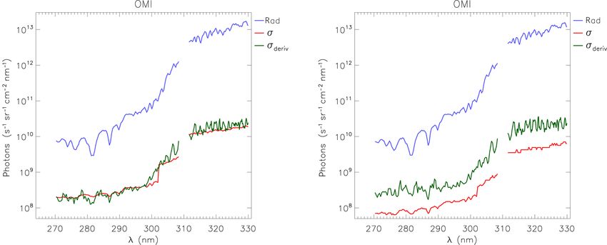
1688                                                             J. C. A. van Peet et al.: Assimilation of UV-VIS ozone profiles

4   Assimilation algorithm                                            with C being the unit conversion (from the models kg grid-
                                                                      cell−1 to the observations DU layer−1 ) and B being the ver-
The assimilation algorithm uses a Kalman filter, and is de-           tical interpolation. The sensitivity matrix H used in Eqs. (9)
scribed in Segers et al. (2005). The state vector x i (i.e. the       and (10) is constructed as H = ABC.
ozone distribution at time t = i) and the measurement vector             In general, the number of elements in an ozone profile is
y i (i.e. the retrieved profiles at time t = i) are given by          much larger than the degrees of freedom (about 5 to 6). We
                                                                      can therefore reduce the number of data points per profile by
x i+1 = M (x i ) + w i ,       wi ∼ N (0, Qi ) ,              (4)     taking the singular value decomposition of the A, and only
y i = H (x i ) + v i ,   v i ∼ N (0, Ri ) ,                   (5)     retain the vectors with a singular value larger than 0.1 (this is
                                                                      an absolute threshold and not relative to the maximum singu-
where M is the model that propagates the state vector in time.        lar value). The profiles and matrices are transformed accord-
It has an associated uncertainty w, which is assumed to be            ingly.
normally distributed with zero mean and covariance matrix                The computational cost of the assimilation algorithm can
Q. The observation operator H , which includes the averaging          be further reduced by minimizing the size of the model
kernel, gives the relation between x and y. The uncertainty in        covariance matrix P. The TM5 model runs in the current
y is given by v, which is also assumed to have zero mean and          setup on a horizontal grid of 2◦ × 3◦ (latitude × longitude)
covariance matrix R (which is identical to Ŝ in the retrieval        on 44 layers, which makes the size of the covariance matrix
equations). In matrix notation, the propagation of the state          (475 200)2 elements. A number of different approaches ex-
vector and its covariance matrix (P) are given by                     ist to minimize the size of the model covariance matrix. For
                                                                      example, in Eskes et al. (2003), the number of dimensions is
x fi+1 = M x ai ,

                                                              (6)     reduced by only assimilating total columns, while the hori-
                                                                      zontal correlation depended only on the distance between the
Pfi+1   = MPai MT   + Qi ,                                    (7)
                                                                      model grid cells. Here, we follow the approach described by
                                                                      Segers et al. (2005), by parameterizing the model covariance
where x f and x a are the forecast and analysis state vectors,
                                                                      into a time-dependent standard deviation field and a constant
respectively, at time t = i, i.e. before and after assimilation of
                                                                      correlation field. At each time step, the model’s advection
the observations. The observations are assimilated according
                                                                      operator is applied to the standard deviation field. The er-
to
                                                                      ror growth (i.e. the addition of Q in Eq. 7) is modelled by
                                                                      a simple mathematical function, more details can be found

x ai = x fi + Ki y i − H x fi ,                                (8)
                                                                      in Sect. 5.2. The model covariance matrix can now be calcu-
Pai = (I − Ki Hi ) Pfi ,                                      (9)     lated according to
                            −1
Ki = Pfi HTi Hi Pfi HTi + Ri     ,                           (10)     P = D (σ ) CD (σ ) ,                                          (12)
                                                                      with D (σ ) being a matrix with the values of the standard
where K is called the Kalman gain matrix, and the matrix H            deviation σ on the diagonal and C the correlation matrix.
is the sensitivity of the observation operator with respect to        The correlation matrix is calculated differently than in Segers
the state.                                                            et al. (2005), more details can be found
                                                                                                              in Sect. 5.3.
    The observation operator interpolates the model field to              Unfortunately, the Hi Pfi HTi + Ri matrix in the Kalman
the observation location, converts the model units to the re-         filter (Eq. 10) is badly conditioned, which makes the inver-
trieval units and takes the smoothing of the satellite instru-        sion sensitive to noise. Therefore, the eigenvalue decompo-
ments into account by incorporating the averaging kernel.             sition of this matrix is calculated and the measurements are
The model grid cells are 3◦ × 2◦ (longitude × latitude), much         projected on the largest eigenvalues, which in total represent
larger than the satellite ground pixels and therefore no hori-        98 % of the original trace of the matrix.
zontal interpolation is needed. The model profile, expressed              For the numerical stability of the assimilation algorithm,
DU layer−1 , is converted to the pressure levels of the re-           the difference between the observation and the model should
trieval grid by applying a simple linear interpolation in the         not be too large. A filter is implemented that rejects the obser-
10 log (hPa) domain. For example, if the L2 profile layer over-       vation when the absolute difference between the observation
laps with three model layers for 20, 100 and 30 %, the inter-         and the model forecast is larger than 3 times the square root
polated model partial column is 0.2 × DU1 + 1.0 × DU2 +               of the sum of the variance in the observation and the variance
0.3 × DU3 (where DUi is the partial column for layer i). Fi-          in the forecast:
nally, the observation operator H is formed by applying the
                                                                                       f
                                                                                                r
averaging kernel A to the difference between the state vector         abs y i − H x i ≥ 3 σy2i + σ 2f ,                            (13)
                                                                                                          xi
x and the a priori profile y a used in the retrieval:
                                                                      with σy and σxf the standard deviation of the observation y
                                                                      and the forecast H (x f ) for layer i, respectively. Note that this

H (x) = A BCx − y a ,                                        (11)

Atmos. Chem. Phys., 18, 1685–1704, 2018                                                 www.atmos-chem-phys.net/18/1685/2018/
J. C. A. van Peet et al.: Assimilation of UV-VIS ozone profiles 1689
is done on a layer-by-layer basis, i.e. if in one layer the dif- where F is the radiance and λ1 the wavelength in detector
ference is too large, the whole observed profile is discarded. pixel 1 and λ2 the wavelength in the adjacent pixel. Because
Not all available ozone profiles can be assimilated into the standard deviation is sensitive to outliers, a Gaussian dis-
TM5 because the computational cost would be too high. Av- tribution is fitted to the data. The fitted standard deviation is
eraging retrievals on the model grid (sometimes called super- multiplied with the spectrum and compared to the reported
observations) was not possible because the assimilation al- noise in the level-1 data.
gorithm described in this paper requires AKs and averaging For GOME-2, we checked 4 days in 2008: 15 March,
AKs is not straightforward. Therefore 1 out of 3 GOME-2 25 June, 26 September and 25 December. On 10 December
profiles and 1 out of 31 OMI profiles are used. These num- 2008 the band 1A/1B boundary was shifted from approxi-
bers are chosen such that more or less the same number of ob- mately 307 to 283 nm and the integration time in this wave-
servations are assimilated for each instrument, taking into ac- length range decreased from 1.5 to 0.1875 s as was already
count the decrease in available pixels due to the row anomaly the case for the rest of band 1B. Therefore, the data for the
in OMI. For OMI, the outermost pixels on each side of the first 3 days are combined, while the data for 25 December
swath are neglected, because of the large area of these pix- is treated separately. The analysis was performed for differ-
els. Of the resulting retrievals, only cloud-free scenes (cloud ent subsets, such as latitude, solar zenith angle and viewing
fraction ≤ 0.2) are assimilated in order to get the maximum angle, but results are shown for latitude only.
amount of information from the troposphere. Figure 1 shows the resulting GOME-2 radiance spectra
for all wavelengths. It should be noted that the these results
are made using spectral data derived from the GOME Data
5 Improvements of the assimilation algorithm Processor (GDP) version 5.3. The older version GDP 4 uses
a different noise model, which yielded too large errors.
The first version of our assimilation algorithm was described The wavelength grid for OMI varies with the location
in Segers et al. (2005). They assimilated GOME ozone pro- across the detector, so the error verification has been per-
files for the year 2000. This dataset was extended to the pe- formed with a dependence on the cross-track position. An
riod 1996–2001 by de Laat et al. (2009) who derived tropo- example radiance spectrum along with the uncertainties is
spheric ozone for this period. The assimilated GOME obser- shown in the left panel of Fig. 2. There is a jump in the spec-
vations in the previous algorithm version had a pixel size of tral uncertainty (the red line) around 300 nm, which might
960 km × 100 km, much larger than the pixels in the current be related to a change in the gain settings for the detector.
research. Since 2009, the assimilation algorithm has been For the selected pixel, the gain changes with a factor of 10 at
further developed and improved for use with GOME-2. The 300 nm.
improved resolution of GOME-2 and OMI ozone profiles and On 1 February 2010, a L0 to L1b processor update
improved retrievals offer new possibilities, but also require was implemented for OMI. The new processor version in-
adaptations in the data assimilation. It is the first time that cludes more detailed information on the row anomaly and
ozone profiles from two nadir looking instruments, GOME-2 a new noise calculation for the three channels UV1, UV2
and OMI, are assimilated simultaneously. This has resulted and VIS. More information can be found on the follow-
in a significant number of updates and improvements to the ing website: http://projects.knmi.nl/omi/research/calibration/
assimilation algorithm compared to the version described in GDPS-History/GDPS_V113.html. The new noise calcula-
Segers et al. (2005) and de Laat et al. (2009), which are out- tion was investigated by taking the radiance differences de-
lined in the following sections. termined a few days after the update. The resulting radiance
spectra are given in the right panel of Fig. 2. The uncertain-
5.1 Observational error characterization ties in the L1 observations after the L0 to L1b processor up-
date are about a factor of 5 smaller than the uncertainties
The covariance matrix of the observations that is used in the
derived according to the method described above.
assimilation is composed of two components, the error on the
In general, the spectral uncertainties for GOME-2 show
spectral observations and the error of the a priori information.
a good agreement with our fitted uncertainties and therefore
Since the spectral errors affect the assimilation results, they
we simply use the uncertainties provided with the observa-
are first verified using the following method.
tions. The spectral uncertainties for OMI show a good agree-
For a given wavelength, two adjacent detector pixels may
ment with our fitted uncertainties before the processor up-
have a radiance or reflectance difference that depends on the
date, but are too small afterwards. The consequences of these
slope of the spectrum. Given enough samples, the standard
smaller uncertainties will be shown in Sect. 6. Since we use
deviation of the mean difference is a good indication of the
the OMI observations as they are, we are not able to correct
noise at that particular wavelength. The relative difference D
for the spectral uncertainties in the retrieval.
is calculated as
F (λ1 ) − F (λ2 )
D= , (14)
0.5 (F (λ1 ) + F (λ2 ))
www.atmos-chem-phys.net/18/1685/2018/ Atmos. Chem. Phys., 18, 1685–1704, 20181690 J. C. A. van Peet et al.: Assimilation of UV-VIS ozone profiles
Figure 1. GOME-2 Metop-A radiance spectra calculated by OPERA: before (a) and after (b) the wavelength shift from 307 to 283 nm. The
blue and red lines are the radiance and uncertainty that are used in OPERA. The green line shows the fitted standard deviations of the relative
difference (see Eq. 14) multiplied by the radiance.
Figure 2. OMI radiance spectrum used in the retrieval, the area around 310 nm is not used. The blue and red lines are the radiance and
uncertainty, respectively. The green line shows the fitted standard deviations of the relative difference (see Eq. 14) multiplied by the ra-
diance. Left plot before the L0 to L1b processor update: date = 25 February 2006, lon = 145.2◦ , lat = −20.3◦ ; right plot after the update:
date = 5 February 2010, lon = 138.0◦ , lat = −28.0◦ .
5.2 Model error growth the layers in the profile, proportional to the partial columns in
each layer (Segers et al., 2005). Deriving a similar relation on
In Sect. 4 we explained that using the full covariance propa- a layer-by-layer basis was not successful, because the error
gation from the Kalman filter equations is too computation- can grow unlimited using this error growth description. Es-
ally intensive. Instead we parameterize the model covariance pecially during the polar night, this might lead to unrealistic
matrix into a time-dependent standard deviation field and high error values.
a time independent correlation field. The advection operator Therefore, we use the following function
is applied to the standard deviation field, and the model error
at
growth is modelled by applying a simple empirical relation. e(t) = , (15)
In the previous version of the assimilation algorithm, the b+t
error growth for the total column was modelled by the func- where a and b are parameters which can be determined by fit-
tion e(t) = At 1/3 (Eskes et al., 2003), with A being a fit pa- ting the observation minus forecast root mean square (RMS)
rameter. The error for the total column was distributed over as a function of time (see Eskes et al., 2003, Fig. 2). The pa-
Atmos. Chem. Phys., 18, 1685–1704, 2018 www.atmos-chem-phys.net/18/1685/2018/J. C. A. van Peet et al.: Assimilation of UV-VIS ozone profiles 1691
Figure 4. Determination of the TM5 correlation field. The solid line
is an assimilation model run, the dashed lines are 10 day free model
runs. After 10 days, there are 11 ozone fields for each given day
which can be used to determine the correlations.
Figure 3. Maximum relative model error (a) as a fraction of the
partial column at different altitudes.
tion length found by Eskes et al. (2003), where total columns
were assimilated instead of profiles.
rameter a is the maximum error of the model at a particular We use a slightly different approach as Segers et al. (2005)
altitude. At t = b, the error is 0.5a, therefore b is a measure because their method neglects uncertainties due to the chem-
of how fast the error grows after a measurement has been as- istry parameterization. Also, the forecast lag of 3 days is
similated. The best results are obtained using b = 2 (days) not compatible with GOME-2 and OMI, which have daily
and let the value of a vary over altitude. The values of a are global coverage. Our reference run is the result of the as-
determined by comparing the free model run (i.e. no assimi- similation of profile observations for April 2008, which we
lation) with all sondes for 2008. Because the model currently consider the true state of the atmosphere. Using the analysis
runs on a 3◦ ×2◦ (longitude × latitude) grid and the sonde ob- field at 00:00 UTC, a model run without assimilation (a free
servations are essentially point sources, these results include model run) is started for a duration of 10 days. After the
a representation error due to the grid-cell size of the model. first 10 days, there are 11 model fields for a given date at
The derived bias is therefore an overestimation of the real 12:00 UTC: 1 from the assimilation run and 10 from the free
model error, and to prevent the model error from increasing model runs (see Fig. 4).
too rapidly all collocations that are more than 3σ from the The difference between the assimilation and free model
mean are discarded. The RMS values of the resulting collo- runs is used to determine the correlations between all pairs of
cations are used as values for a, they are shown as relative grid cells in the vertical direction (constant location), in the
values in Fig. 3 for comparison over different altitudes. For East–West direction (constant latitude and altitude), and in
the error of the layers above the maximum altitude of the the North–South direction (constant longitude and altitude).
sondes (about 5 hPa), a has been set to the same value as the The correlations are determined as a function of the distance.
last layer below the maximum altitude. Since the East–West distance between two grid cells is larger
at the equator than near the poles, the East–West correlation
5.3 Model correlation matrix also depends on the latitude. The calculated correlations as
a function of distance are fitted with a Gaussian distribution
In order to calculate the time independent correlation field, (with correlations less than 0.01 set to zero). Both the calcu-
we follow the National Meteorological Center’s method lated and fitted correlations are shown in Fig. 5. The fitted
(NMC-method) to determine the correlation in the model correlations are used in subsequent model runs as the time
(see Parrish and Derber, 1992; Segers et al., 2005). Segers independent correlation field.
et al. (2005) used a reference run based on 6-hourly meteo-
rological forecasts as the starting point for forecast runs that 5.4 Ozone profile error characterization and bias
last 9 days and start at 12:00 UTC. After a spin-up period, correction
9 forecast fields per day are available which can be used to
determine the correlation in ozone. Differences between the The biases between two instruments should be as small as
ozone concentration in these runs are due to the different me- possible for a stable assimilation. Therefore, a bias correc-
teorological inputs. Since the overpass frequency of GOME tion as a function of solar zenith angle (SZA), viewing angle
is 3 days, the forecast field from the run started 3 days be- (VA) and time has been developed based on the results of the
fore the current date was used to derive the correlations in comparison with sondes. The bias correction factor is one
the ozone field. This choice also best matched the correla- minus the median of the relative deviation based on all col-
www.atmos-chem-phys.net/18/1685/2018/ Atmos. Chem. Phys., 18, 1685–1704, 20181692 J. C. A. van Peet et al.: Assimilation of UV-VIS ozone profiles Figure 5. Calculated (a, c, e) and fitted (b, d, f) correlations for the latitudinal (a, b), surface layer longitudinal (c, d) and vertical (e, f) directions. located data in a given year. All observations in a given year tics are the following. Only cloud-free (cloud fraction < 0.2) are multiplied by this correction factor. retrievals have been used, the sonde launch location should Figure 6 shows the global validation results for the 4 years be located in the pixel footprint, and the satellite overpass of the assimilation period (2008–2011) of the GOME-2 and time should be within 3 h of sonde launch. When multiple OMI profiles with ozone sondes downloaded from the World retrievals collocate with the same sonde, only the one clos- Ozone and Ultraviolet Radiation Data Centre (WOUDC, est in time has been used. The collocated sonde profiles have WMO/GAW, 2016). The validation methodology has been been interpolated on the pressure grid of the retrievals and described in van Peet et al. (2014), and the main characteris- extended to the top of the atmosphere with the a priori pro- Atmos. Chem. Phys., 18, 1685–1704, 2018 www.atmos-chem-phys.net/18/1685/2018/
J. C. A. van Peet et al.: Assimilation of UV-VIS ozone profiles                                                                          1693

Figure 6. Global validation results for 2008–2011 for GOME-2 (a, b) and OMI (c, d). (a, c) show the median absolute differences, (b, d)
show the median relative differences. The blue line indicates the original observations, the red line the bias corrected observations that have
been used as input for the assimilation. The error bars indicate the range between the 25 and 75 % percentiles. Note that the x axis scale is
different for each plot.

file above the burst level of the sonde. The interpolated and             of which 33 reached the top level. Table 1 lists all stations
extended profiles are convolved with the averaging kernels                and the number of sondes used in the validation and bias cor-
in order to take the vertical sensitivity of the satellite instru-        rection of the observations. The numbers in the station names
ments into account.                                                       refer to the WOUDC station identifiers.
   The bias of GOME-2 with respect to sondes varies be-
tween −1.1 and +1.7 DU (−7 and +7 %) between 100 and
10 hPa, while for altitudes below 100 hPa the bias is about               6   Results and validation
−0.3 DU (−4 %). The bias of OMI varies between −4.5 and
                                                                          We have assimilated GOME-2 (on Metop-A) and OMI ozone
+2 DU (−8 and +15 %) between 100 and 10 hPa, while be-
                                                                          profiles for a period of 4 years between 2008 and 2011 us-
low 10 hPa the bias is positive with a maximum value of
                                                                          ing the Kalman filter algorithm described in the previous
4 DU (+27 %). The absolute biases cannot be compared di-
                                                                          sections. In total, four model runs were performed: a “free”
rectly because the layers of GOME-2 and OMI do not have
                                                                          model run without assimilation, a model run with assimila-
the same thickness. Note that the remaining biases for the top
                                                                          tion of GOME-2 ozone profiles only, a model run with as-
layers in Fig. 6 are not exactly zero for the corrected obser-
                                                                          similation of OMI ozone profiles only and a model run with
vations, because the figure is drawn for latitude bands, while
                                                                          simultaneous assimilation of GOME-2 and OMI ozone pro-
the bias correction is made using SZA and VA bins and the
                                                                          files.
number of sondes used in the comparison at that altitude is
much smaller than at lower altitudes. For the validation of
GOME-2, 1083 sondes were used, of which 10 reached the
top level. For the validation of OMI, 776 sondes were used,

www.atmos-chem-phys.net/18/1685/2018/                                                       Atmos. Chem. Phys., 18, 1685–1704, 2018
1694 J. C. A. van Peet et al.: Assimilation of UV-VIS ozone profiles
Table 1. Stations used for the validation and bias correction of GOME-2 and OMI.
Station long. lat. # GOME-2 # OMI
stn_018_alert −62.33 82.50 32 0
stn_021_edmonton-stony_plain −114.11 53.55 0 4
stn_024_resolute −94.97 74.71 27 1
stn_029_macquarie_island 158.94 −54.50 14 0
stn_043_lerwick −1.19 60.14 31 26
stn_053_uccle 4.35 50.80 66 43
stn_055_vigna_di_valle 12.21 42.08 3 1
stn_076_goose_bay −60.36 53.31 17 0
stn_089_ny_alesund 11.95 78.93 35 9
stn_101_syowa 39.58 −69.01 0 4
stn_107_wallops_island −75.47 37.93 28 23
stn_109_hilo −155.04 19.43 34 0
stn_156_payerne 6.57 46.49 153 156
stn_174_lindenberg 14.12 52.21 30 36
stn_175_nairobi 36.80 −1.27 25 10
stn_191_samoa −170.56 −14.23 42 3
stn_199_barrow −156.60 71.30 12 14
stn_219_natal −35.26 −5.49 0 27
stn_221_legionowo 20.97 52.40 39 33
stn_233_marambio −56.62 −64.24 23 2
stn_242_praha 14.44 50.00 29 48
stn_256_lauder 169.68 −45.04 4 7
stn_308_madrid-barajas −3.58 40.47 59 52
stn_315_eureka-eureka_lab −85.94 79.99 56 1
stn_316_debilt 5.18 52.10 40 29
stn_318_valentia_observatory −10.25 51.93 37 19
stn_323_neumayer −8.26 −70.65 63 11
stn_328_ascension_island −14.42 −7.98 0 10
stn_330_hanoi 105.80 21.01 0 4
stn_336_isfahan 51.70 32.51 0 1
stn_338_bratts_lake-regina −104.70 50.20 24 37
stn_339_ushuaia −68.31 −54.85 6 2
stn_344_hong_kong_observatory 114.17 22.31 4 28
stn_348_ankara 32.86 39.97 0 9
stn_394_broadmeadows 144.95 −37.69 36 29
stn_434_san_cristobal −89.62 −0.92 1 0
stn_435_paramaribo −55.21 5.81 33 0
stn_436_la_reunion_island 55.48 −21.06 20 11
stn_437_watukosek-java 112.60 −7.50 3 4
stn_438_suva_fiji 178.40 −18.13 6 3
stn_443_sepang_airport 101.70 2.73 6 0
stn_445_trinidad_head −124.20 40.80 5 5
stn_450_davis 77.97 −68.58 5 12
stn_456_egbert −79.78 44.23 22 13
stn_457_kelowna −119.40 49.94 0 24
stn_466_maxaranguape-shadoz-nat −35.26 −5.49 0 25
stn_477_heredia −84.11 10.00 2 0
stn_494_alajuela −84.21 9.98 11 0
total 1083 776
Atmos. Chem. Phys., 18, 1685–1704, 2018 www.atmos-chem-phys.net/18/1685/2018/J. C. A. van Peet et al.: Assimilation of UV-VIS ozone profiles 1695
Figure 7. GOME-2 OmF (blue) and OmA (red) for the surface layer (a), around 10 hPa (b and c) and around 0.3 hPa (d). The OmF and
OmA have been calculated for the regridded layers from the model run with simultaneous assimilation of GOME-2 and OMI.
6.1 Altitude dependent OmF and OmA statistics to hPa and correspond to surface pressure up to 0.28 hPa.
The observation minus analysis (OmA) is defined in a similar
An important diagnostic of any assimilation system is the dif- way, but with x f replaced with the analysis profile x a . Since
ference between the observations and the model (also known the analysis field is a weighted average of the forecast model
as innovations). In the following, we define the relative ob- field and the observations, the OmA should be smaller than
servation minus forecast (OmF) for layer i as the OmF.
y i − H x fi
In Fig. 7, the GOME-2 OmF and OmA from the model
OmFi = , (16) run with simultaneous assimilation of GOME-2 and OMI for
0.5 y i + H x fi four different layers have been plotted. The ozone sondes that
with i the layer index, y the observed ozone profile, H the were used in deriving the bias correction and the validation
observation operator and x f the forecast profile of the model of the results were required to have reached at least 10 hPa.
(see Sect. 4). The layers in the retrievals of GOME-2 and Therefore the selected layers in Fig. 7 are the surface layer,
OMI have a different thickness, which makes the compari- the layer just below and above 10 hPa, and the top layer of
son of the OmF between the two instruments not straight- the new pressure grid around 60 km (0.3 hPa). In Fig. 8, the
forward. Therefore, both y and H x f have been regridded OmF and OmA for the same layers have been plotted for
to the same pressure levels before calculating the OmF. This OMI. In the first year of the assimilation period, the surface
new vertical grid is defined by levels at 0, 6 and 12 km fol- layer OmF and OmA for GOME-2 are higher than those for
lowed by levels every 2 up to 60 km, which are converted OMI. At the end of 2008, after the wavelength shift between
www.atmos-chem-phys.net/18/1685/2018/ Atmos. Chem. Phys., 18, 1685–1704, 20181696 J. C. A. van Peet et al.: Assimilation of UV-VIS ozone profiles Figure 8. OMI OmF (blue) and OmA (red) for the surface layer (a), around 10 hPa (b and c) and around 0.3 hPa (d). The OmF and OmA have been calculated for the regridded layers from the model run with simultaneous assimilation of GOME-2 and OMI. GOME-2 band 1A/1B, the situation is reversed and the OmF layer, the OmF and OmA for GOME-2 are about 5 percent- and OmA for GOME-2 are lower than those for OMI. The age points higher than for OMI. In general, the OmF is about band 1A/1B wavelength shift is clearly present in the bottom 2–4 percentage points higher than the OmA, except for the layer of the GOME-2 OmF and OmA, which might be unex- top layer. There, the difference is in the order of 1 percent pected since the radiation from band 1A/1B does not reach point, but the values vary much more than lower in the atmo- the surface. But since the layers in an optimal estimation re- sphere. trieval are related as described by the AK and covariance ma- Both OmF and OmA for the GOME-2 assimilation run trices, it is possible that the band 1A/1B change affects the show regular decreases with a period of about 1 month. results in an altitude region where the radiation itself does not These decreases are caused by GOME-2 being operated in penetrate. The OMI data show a more pronounced yearly cy- “narrow-swath mode”, when the swath is 320 km wide in- cle than GOME-2. After the beginning of 2010, the OmF and stead of 1920 km. For these narrow-swath observations, the OmA for both instruments are very similar for the summer model is closer to the retrieved profiles, causing a lower months June, July and August, but the winter time values for OmF/OmA. OMI also has a spatial zoom-in mode, which is OMI are higher. For the layer just below 10 hPa, the OmF and activated about once a month, but these pixels are filtered out OmA for GOME-2 are about 1 percentage point higher than because they are too much influenced by the row anomaly for OMI. For the layer just above 10 hPa, the OmF and OmA and because the mapping between the UV-1 and UV-2 pixels for GOME-2 start out lower than for OMI, but at the end of change with respect to the normal mode. Peaks in the OmF the assimilation period the values are comparable. For the top and OmA for the GOME-2 assimilation, such as after an in- Atmos. Chem. Phys., 18, 1685–1704, 2018 www.atmos-chem-phys.net/18/1685/2018/
J. C. A. van Peet et al.: Assimilation of UV-VIS ozone profiles                                                                1697

                                                                        Lower uncertainties in the spectra lead to lower uncertain-
                                                                     ties in the observations, which in its turn changes the balance
                                                                     between model and observations in the Kalman filter and af-
                                                                     fects the innovations. Because the variance in the observa-
                                                                     tion is lower, more pixels will be rejected by the OmF filter
                                                                     (see Sect. 4 and Fig. 10). Figure 10 shows the number of as-
                                                                     similated observations for both GOME-2 and OMI from the
                                                                     single and simultaneous instrument assimilation. In the sin-
                                                                     gle instrument assimilation runs, the model error is adapted
                                                                     to the new situation after the processor update and the to-
                                                                     tal number of assimilated observations does not change. For
                                                                     the simultaneous assimilation, the assimilation results may
                                                                     be fluctuating between OMI and GOME-2 observations if
                                                                     a bias exists. This might result in higher assimilation errors.
                                                                     Therefore, the OmF filter (see Sect. 4 and Eq. 13) rejects ob-
                                                                     servations from both GOME-2 and OMI, even though only
Figure 9. OMI OmF (blue) and OmA (red) for the layer around
0.3 hPa, zoomed in to a month before and after the L0 to L1b pro-
                                                                     the uncertainties from one of the instruments (i.e. OMI) have
cessor update. The OmF and OmA have been calculated for the          changed.
regridded layers from the model run with simultaneous assimilation
of GOME-2 and OMI.                                                   6.2   Altitude independent OmF and OmA statistics

                                                                     In order to show the geographical distribution of the OmF
strument test period between 7 and 12 September 2009, can            and OmA, the absolute values for each layer were quadrat-
be related to periods of missing data.                               ically added and the square root was taken from the result.
   Sudden changes in the OmF and OmA are visible for some            These column-integrated OmF and OmA values were aver-
altitudes for both instruments at the start of some years. One       aged on a daily basis for latitude bins with a size of 2◦ . In
example is in the layer just above the 10 hPa for GOME-2 at          Fig. 11, these column-integrated OmF and OmA are shown
the start of 2009 or at the start of 2010 for OMI. The change        as a function of latitude and time. The highest values of the
for GOME-2 appears to coincide with the band 1A/1B shift,            OmF and OmA are observed at high latitudes around the po-
but it is really at the start of the year and not on 10 Decem-       lar night. The GOME-2 band 1A/1B wavelength change is
ber 2008. It is therefore unlikely that these two events are         clearly visible, even though the plot shows OmF and OmA
related. Since there are no known instrumental or meteoro-           from the combined assimilation. Step changes in the OmA
logical changes, the most likely cause is therefore the bias         are visible at the start of each year, which coincides with an
correction scheme for the observations, which changes its            update of the bias correction parameters.
correction parameters at the start of each year.
   Closer inspection of the OMI OmF and OmA change at the            6.3   Expected and observed OmF
start of 2010 (see the lower left panel of Fig. 8), shows that it
actually consists of two steps: the first one at the start of the    The OmF of the results should be consistent with the un-
year and the second one a month later. That second step is           certainties of the observations and the model forecast. The
also present in Fig. 8d (the layer around 0.3 hPa), where the        expected OmF is based on the observation error and the fore-
change is about 5 percentage points, but it is less clear due to     cast error and is the mean of the square root term in the right-
the higher variability in the signal. Figure 9 shows the same        hand side of Eq. (13) for all observations in a given layer. The
data, but focused on the first two months of 2010. Both OmF          observed OmF for each layer for the whole assimilation pe-
and OmA increase by about 5 percentage points from one               riod, on the other hand, is the mean of the left-hand side of
day to the next. The increase is even larger (and more clearly       Eq. (13). In Fig. 12, the observed OmF is plotted as a function
visible) in the data from the single instrument assimilation         of the expected OmF for the model runs with assimilation of
run for OMI.                                                         GOME-2 only with assimilation of OMI only, and for both
   Comparison of Figs. 7 and 8 shows that the OmF and OmA            instruments separate with the data taken from the model run
for one instrument might be larger than for the other, depend-       with simultaneous assimilation.
ing on the altitude. Which of the two instruments has a larger          Note that the pressure levels are those from the observa-
OmF or OmA value might also change over time. In other               tions, not the regridded levels used in the calculation of the
words, GOME-2 and OMI have a different sensitivity for               OmF and OmA above. The expected and observed OmF are
different altitudes as represented by the averaging kernels.         close to the 1-to-1 line, which shows that the model error
Assimilating the observations from these instruments simul-          σx f is of the correct magnitude for the current observations.
taneously increases the overall sensitivity of the assimilation.     The expected and observed OmF are somewhat closer to the

www.atmos-chem-phys.net/18/1685/2018/                                                 Atmos. Chem. Phys., 18, 1685–1704, 2018
1698 J. C. A. van Peet et al.: Assimilation of UV-VIS ozone profiles
Figure 10. Number of assimilated observations from GOME-2 (a) and OMI (b). The blue lines represent the single instrument assimilation,
the red lines the simultaneous assimilation.
Figure 11. Mean OmF (a) and OmA (b) as a function of latitude (bin size 2◦ ) and time (bin size 1 day) for the simultaneous assimilation of
GOME-2 and OMI.
1-to-1 line in the case of the simultaneous assimilation of all observations are corrected with the same factor. The as-
GOME-2 and OMI than for the assimilation of each instru- similation model runs are significantly better than the free
ment independently. The model error that is used is therefore model run. This is especially true for the part of the atmo-
probably slightly better suited for the assimilation of multi- sphere where GOME-2 and OMI are most sensitive to the
ple instruments simultaneously than for the assimilation of ozone concentration, between 100 and 10 hPa. In this area,
a single sensor. the model run with assimilation of GOME-2 only shows
a negative bias with respect to the ozone sondes, while the
6.4 Assimilation validation with sondes assimilation of OMI shows a positive bias. The assimilation
of both GOME-2 and OMI shows the smallest bias. The de-
The model output was validated against ozone sondes that viation in the differences are very similar for the four runs,
were obtained from the World Ozone and Ultraviolet Radia- which is why only the error bars for the simultaneous assimi-
tion Data Centre (WOUDC, WMO/GAW, 2016, see Fig. 13). lation have been plotted in Fig. 13. The 25–75 percentile dif-
This is the same ozone dataset as was used to derive the bias ferences are in the 20–55 percentage points range between 0
correction. Note, however, that many more observations are and 20 km and in the 10–20 percentage points range between
assimilated than were used deriving the bias correction, while 20 and 40 km.
Atmos. Chem. Phys., 18, 1685–1704, 2018 www.atmos-chem-phys.net/18/1685/2018/J. C. A. van Peet et al.: Assimilation of UV-VIS ozone profiles 1699 Figure 12. Observed vs. expected OmF. (a) Assimilation of GOME-2 only, (b) assimilation of OMI only. (c, d) Results from the simultaneous assimilation of both GOME-2 and OMI. (c) GOME-2, (d) OMI. Colours indicate the pressure levels. Note that not all levels are plotted in the legend while all levels are plotted in the figure. The size of the circles gives the number of assimilated pixels (n) in that respective OmF-bin (bin-size = 0.2 DU). The slope for the fitted (dashed) line is given in the lower right corner of each panel, as is the correlation (R) between the expected and observed OmF. In the troposphere, the assimilation also improves, but increasing bias above 10 hPa, it should be noted that the num- not as much as in the stratosphere. Note that in the tropo- ber of sondes reaching this altitude is limited with respect sphere the chemistry scheme is different than in the strato- to the tropopause region between 200 and 100 hPa. Also, sphere (see Sect. 3). The assimilation shows a deviation in there is a representation error of the sonde with respect to the tropopause, between 200 and 100 hPa, although the L2 the 3◦ longitude × 2◦ latitude model grid. Therefore it is not data do not show such large biases (see Fig. 6). The verti- as straightforward to attribute this increase in bias to either cal resolution of model and observation is different, there- model or observation error. fore the ozone from the observation has to be redistributed over the model layers, a process which is included in the operator H . A small error in the redistribution of ozone in 7 Case study a region with a strong gradient in the concentration (such as the tropopause) will result in large uncertainties in the To demonstrate the performance of the assimilation algo- ozone concentration at this altitude. Above 10 hPa the assim- rithm we analysed the results for a day above the Tibetan ilation shows increasing biases, and the difference with the Plateau (located between 30 and 40◦ N), where a highly free model run decreases. Although the L2 data also show an dynamical atmosphere exists. This makes it an interesting www.atmos-chem-phys.net/18/1685/2018/ Atmos. Chem. Phys., 18, 1685–1704, 2018
1700                                                              J. C. A. van Peet et al.: Assimilation of UV-VIS ozone profiles

Figure 13. Validation of the model runs with ozone sondes for 2008–2011. (a) The median of the absolute difference in DU, (b) the median
of the relative differences. Blue: model run without assimilation, green: model run with assimilation of GOME-2 only, yellow: run with
assimilation of OMI only, red: assimilation of both GOME-2 and OMI. The error bars are plotted for the simultaneous assimilation only, and
range from the 25 to the 75 % percentile.

Figure 14. Two meridional cross sections over the Tibetan Plateau, located at 84.25◦ E on 25 February 2008, 06:00 UTC. The colours indicate
the ozone concentration from the free model run (a) and the assimilation of both GOME-2 and OMI (b). The solid contours show the ozone
concentrations from the ERA-Interim reanalysis. The dashed line shows the thermal tropopause.

area to study atmospheric dynamics, and difficult for mod-              35◦ N at pressure levels between 70 and 10 hPa. Even though
elling so it can serve as a test case to see if the dynamics in         the GOME-2 and OMI instruments have limited sensitivity in
the model are correctly implemented. On 25 February 2008                the troposphere, the tropospheric ozone concentrations of the
a stratosphere–troposphere exchange event was observed in               ERA-Interim reanalysis and assimilated tropospheric ozone
GOME-2 data (Chen et al., 2013), which can also be ob-                  are in better agreement north of the Tibetan Plateau. There
served in the assimilation output. In Fig. 14, ozone concen-            are also two stratosphere–troposphere exchanges (STE) vis-
trations from the ERA-Interim reanalysis (Dee et al., 2011;             ible, at 30 and 60◦ N. These STEs are associated with strong
Dragani, 2011) are plotted as contours over the ozone con-              jet-streams (perpendicular to the page) reaching wind speeds
centrations from the model runs with and without simulta-               of up to 50 m s−1 at 250 hPa.
neous assimilation of GOME-2 and OMI. There is a signif-
icantly better agreement between the two datasets north of

Atmos. Chem. Phys., 18, 1685–1704, 2018                                                   www.atmos-chem-phys.net/18/1685/2018/
J. C. A. van Peet et al.: Assimilation of UV-VIS ozone profiles                                                            1701

8   Discussion                                                       The model covariance matrix is also an expensive step in
                                                                  the assimilation algorithm. We have reduced the calculation
                                                                  cost by parameterizing it into a time-dependent error field
When two instruments are assimilated simultaneously, their        and a time-independent correlation field. The data from April
differences should be taken into account. For example, the        2008 was used to derive the correlations, which were then
algorithms used for the retrieval of GOME-2 and OMI ozone         used for the whole assimilation period. The assumption that
profiles both produce partial columns. However, the num-          the derived correlations are constant throughout time has not
ber of layers in the retrievals differ and the sensitivity of     been tested.
the retrieval is expressed by the averaging kernel. Both the
different vertical resolution and the averaging kernel are in-
corporated into the observation operator H . Both instruments     9   Conclusions
have different horizontal resolution, something which has not
been taken into account in the current version of the assim-      An algorithm for the simultaneous assimilation of GOME-
ilation algorithm. The measurement principle of GOME-2            2 and OMI ozone profiles has been described. The algo-
(i.e. a cross-track scanning mirror) is different than that of    rithm uses a Kalman filter to assimilate the ozone profiles
OMI (i.e. a fixed 2-D CCD detector). As a result, the ground      into the TM5 chemical transport model. Compared to pre-
pixel size of GOME-2 is constant, while that of OMI varies        vious versions, the algorithm is significantly updated. The
across the track. Therefore, the representation error of OMI      observational error has been characterized using a newly de-
will increase towards the edges of the swath. The effect of       veloped in-flight calibration method. Since the Kalman fil-
the changing OMI footprint size has not been investigated.        ter equations are too expensive to calculate directly for the
To get an idea of the sub-grid-cell variation in the ozone con-   current setup, the model covariance matrix is divided into
centration, we performed a small experiment where we as-          a time-dependent error field and a time independent corre-
similated the same observations (i.e. GOME-2 and OMI) into        lation field. The time evolution is applied to the error field
TM5 running on a 1◦ × 1◦ grid (as opposed to the standard         only, while the correlation is assumed to be constant. The
3◦ × 2◦ used in this article). The total column standard devi-    model error growth is modelled by a new function that pre-
ation of the six 1◦ × 1◦ grid cells covered by a single 3◦ × 2◦   vents the error from increasing indefinitely, and the correla-
grid cell is much smaller than the error on the total column.     tion field has been newly derived using the NMC method.
Therefore, the representation error due to the large grid cells   Large biases between retrievals of the two instruments might
is not significant. A more thorough check on the instruments      destabilize the assimilation. To avoid this, a bias correction
behaviour throughout time might have revealed the effect of       using global ozone sonde observations has been applied to
the OMI L0 to L1b processor update sooner. The threshold          the retrieved ozone profiles before assimilation.
of the parameter in the OmF filter might be made instrument          Four model runs were performed spanning the years be-
and time dependent in order to minimize the effect on the         tween 2008 and 2011: without assimilation, with assimila-
number of assimilated pixels.                                     tion of GOME-2 only, with assimilation of OMI profiles only
   Two different instruments can be biased with respect to        and with simultaneous assimilation of both GOME-2 and
each other. In order to minimize the bias, a bias correction      OMI profiles. Depending on the altitude, the OmF and OmA
scheme has been implemented with respect to ozone sondes.         for one instrument might be larger than the other, which
We used cloud-free observations (max. cloud fraction 0.20)        might change in the course of time. Assimilating the ob-
for the bias correction in order to get a maximum amount          servations from these instruments simultaneously increases
of information from the troposphere. As a consequence, we         the overall sensitivity of the assimilation. Two notable in-
could not use all available sondes in deriving the bias cor-      strumental effects are the band 1A/1B wavelength shift for
rection. Sudden changes in the bias correction parameters         GOME-2, which causes a significant decrease in OmF and
are visible at the start of the year, when the parameters are     OmA. For OMI, after the L0 to L1b processor update on
changed. To minimize these changes, it might be worthwhile        1 February 2010, the uncertainty in the observations is too
to implement an interpolation scheme for the bias correction      small with respect to the method of in-flight validation of the
parameters similar as for the MSR data (see van der A et al.,     uncertainties presented in this paper. This caused a decrease
2010, 2015).                                                      in the number of assimilated observations for both GOME-
   The model can run a full chemistry scheme, but instead         2 and OMI. The expected and observed OmF and OmA are
a parameterized chemistry scheme has been used in favour          more similar for the combined assimilation than for the sepa-
of speed. Another possibility to increase the accuracy of the     rate assimilations. Validation with sondes from the WOUDC
model is to increase the horizontal resolution from the cur-      shows that the combined assimilation performs better than
rent 3◦ × 2◦ (long. × lat.) to 1◦ × 1◦ for example. However,      the single sensor assimilation in the region between 100 and
in both cases it might be necessary to reduce the vertical res-   10 hPa where GOME-2 and OMI are most sensitive. The
olution of the model to keep the computational cost at an         ozone concentrations in the troposphere are also affected by
acceptable level.                                                 the assimilation, even though the instruments have limited

www.atmos-chem-phys.net/18/1685/2018/                                              Atmos. Chem. Phys., 18, 1685–1704, 2018
You can also read