An Empirical Comparison of Machine-Learning Methods on Bank Client Credit Assessments - MDPI
←
→
Page content transcription
If your browser does not render page correctly, please read the page content below
sustainability

Article
An Empirical Comparison of Machine-Learning
Methods on Bank Client Credit Assessments
Lkhagvadorj Munkhdalai 1 , Tsendsuren Munkhdalai 2 , Oyun-Erdene Namsrai 3 ,
Jong Yun Lee 1, * and Keun Ho Ryu 4, *
 1    Database/Bioinformatics Laboratory, College of Electrical and Computer Engineering,
      Chungbuk National University, Cheongju 28644, Korea; lhagii@dblab.chungbuk.ac.kr
 2    Microsoft Research, Montreal, QC H3A 3H3, Canada; tsendsuren.munkhdalai@microsoft.com
 3    Department of Information and Computer Sciences, National University of Mongolia, Sukhbaatar District,
      Building#3 Room#212, Ulaanbaatar 14201, Mongolia; oyunerdene@seas.num.edu.mn
 4    Faculty of Information Technology, Ton Duc Thang University, Ho Chi Minh City 700000, Vietnam
 *    Correspondence: jongyun@chungbuk.ac.kr (J.Y.L.); khryu@tdtu.edu.vn (K.H.R.);
      Tel.: +82-43-261-2789 (J.Y.L.); +82-10-4930-1500 (K.H.R.)

 Received: 17 December 2018; Accepted: 21 January 2019; Published: 29 January 2019

 Abstract: Machine learning and artificial intelligence have achieved a human-level performance
 in many application domains, including image classification, speech recognition and machine
 translation. However, in the financial domain expert-based credit risk models have still been
 dominating. Establishing meaningful benchmark and comparisons on machine-learning approaches
 and human expert-based models is a prerequisite in further introducing novel methods. Therefore,
 our main goal in this study is to establish a new benchmark using real consumer data and to
 provide machine-learning approaches that can serve as a baseline on this benchmark. We performed
 an extensive comparison between the machine-learning approaches and a human expert-based
 model—FICO credit scoring system—by using a Survey of Consumer Finances (SCF) data. As the
 SCF data is non-synthetic and consists of a large number of real variables, we applied two
 variable-selection methods: the first method used hypothesis tests, correlation and random
 forest-based feature importance measures and the second method was only a random forest-based
 new approach (NAP), to select the best representative features for effective modelling and to compare
 them. We then built regression models based on various machine-learning algorithms ranging from
 logistic regression and support vector machines to an ensemble of gradient boosted trees and deep
 neural networks. Our results demonstrated that if lending institutions in the 2001s had used their
 own credit scoring model constructed by machine-learning methods explored in this study, their
 expected credit losses would have been lower, and they would be more sustainable. In addition, the
 deep neural networks and XGBoost algorithms trained on the subset selected by NAP achieve the
 highest area under the curve (AUC) and accuracy, respectively.

 Keywords: automated credit scoring; decision making; machine learning; internet bank; sustainability

1. Introduction
     For lending institutions, credit scoring systems aim to provide probability of default (PD) for
their clients and to satisfy a minimum-loss principle for their sustainability. Therefore, a credit
scoring system supports decision making for credit applications, manages credit risks and influences
the amount of non-performing loans that are likely to lead to bankruptcy, financial crisis and
environment sustainability.
     In the last decade, although credit officers or expert-based credit scoring model determine
whether borrowers can fulfill their requirements, it has changed over time with technological advances.

Sustainability 2019, 11, 699; doi:10.3390/su11030699                      www.mdpi.com/journal/sustainability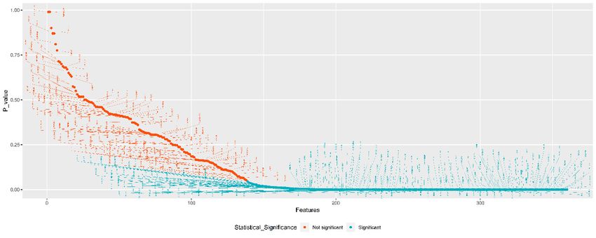
Sustainability 2019, 11, 699                                                                          2 of 23

This change needs the establishment of an automated credit decision-making system that can avoid
loss of opportunity or credit losses to reduce potential loss for each lending institution. Therefore,
in recent years, automated credit scoring has become very crucial because of the growing number
of financial services without human involvement. An example of such financial services is the
recent establishment of the first internet-only banking firm in South Korea [1]. In other words, the
use of technology and automation to reduce the operating costs for modern lending institutions
requires the development of an accurate credit scoring model. Although it is extremely difficult to
perform an efficient model for estimating clients’ creditworthiness, machine learning now plays a vital
role in credit scoring application. A line of work has studied automated credit scoring as a binary
classification problem in the machine-learning context. Existing studies have incorporated the use of
data-mining techniques and machine-learning algorithms such as Discriminant analysis [2], Neural
networks [3], Support vector machine [4], Decision trees [5], Logistic regression [6], Fuzzy logic [7],
Genetic algorithm [8], Bayesian networks [9], Hybrid methods [10,11] and Ensemble methods [12].
In addition, numerous authors have proposed different feature-selection methods for credit scoring
such as wrapper-feature-selection algorithms [13], Wald statistic using chi-square test [14], evolutionary
feature selection with correlation [15], hybrid feature-selection methods [16] and multi-stage feature
selection based on genetic algorithm [17].
       Unfortunately, the prior work focused only on their performance in binary credit classification.
It is inefficient and not practical from the perspective of the banking risk management. The result of
predictive accuracy of the estimated PD can be more valuable and expressive than the output of the
binary classifier, i.e., credible or not credible clients [18]. Furthermore, the regulatory organizations for
lending institutions require PDs with internal ratings or credit ratings than performance in the simple
binary credit classification. For example, if lending institutions follow the International Financial
Reported Standards (IFRS), they have to perform a multi-class credit rating to assess the PD and loss
given default (LGD) for loan loss provisions on each credit rating [19] as well as the international
committee of banking supervisory authorities that the Basel Committee recommends to perform
internal credit ratings [20].
       In addition, the previous studies mainly built upon the German (1994), Australian (1992), Japanese
(1992) and other available datasets [21]. Louzada [22] found that nearly 45% of all reviewed papers
relating on the theory and application of binary credit scoring used the Australian or German credit
dataset. Although these datasets can be viewed as benchmarks in artificial intelligence, they do not
represent a realistic setup as they have a limited number of variables and without such the realistic
data established for benchmarking. It is nontrivial to provide a direct comparison between machine
learning and expert-based models. More recently, Xia [23] also highlighted that finding other public
datasets in credit scoring problem is still difficult. This fact indicates that how difficult is to obtain
datasets on the credit scoring scenario since there are issues related to maintenance of confidentiality
of credit scoring databases.
       However, a small number of studies used real-life credit scoring dataset, but these datasets are not
available for retrieving and analyzing [24–27]. For example, in accordance to bank managers’ expert
opinions in Taiwan, Chen [24] discussed the evaluation and selection factors for client credit granting
quality and adopts Decision-Making Trial and Evaluation Laboratory to compare and analyze the
similarities and the differences in a bank’s evaluation for client traits, abilities, financial resources,
collaterals, and other dimensions (criteria). Dinh [25] developed econometric credit scoring model
using Vietnam’s commercial banks dataset. Jacobson [26] proposed a method to estimate portfolio
credit risk using bivariate probit regression based on Swedish consumer credit dataset.
       To summarize, although many studies have been applied various machine-learning algorithms
for credit scoring, none of them compared their performances to human expert-based models because
available benchmark dataset for this comparison is rare. However, establishing meaningful benchmark
and comparisons on machine-learning approaches and human expert-based models have to be
prerequisite in further introducing novel methods.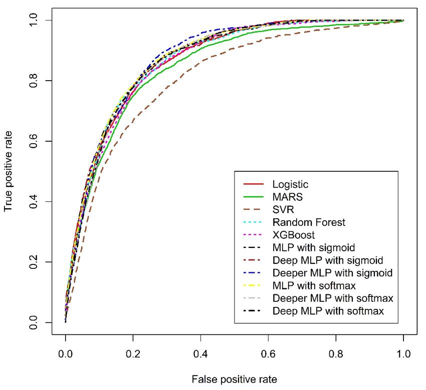
Sustainability 2019, 11, 699                                                                        3 of 23

      In this study, our main goal is to establish a new benchmark using real consumer data and
to provide machine-learning approaches that can serve as a baseline on this benchmark. Then the
contribution of this study is to introduce a more realistic setting in order to fill the gap between
experimental studies from the literature and the demanding needs of the lending institutions.
To overcome this, an open source dataset as a benchmark to compare credit scoring applications
in the real world is explored. The existing credit scoring system and the evaluation metric for
comparison are demonstrated as well. More specifically, we explored a Survey of Consumer Finances
(SCF) data, which is a U.S. families’ survey retrieved from The Federal Reserve [28]. SCF dataset
contains a large number of variables which consists of a variety of useful information that can directly
be interpreted into a credit scoring system such as types of credit used, credit history, demographics,
attitudinal, income, capital gains, expenditures, assets, etc. [29]. Description of variables is given as
Supplementary Material.
      Since we use SCF data come from the U.S. population to construct machine-learning based-credit
scoring models, FICO credit scores—the industry standard for measuring consumer credit risk in the
U.S. [30]—can be compared to them. However, in order to perform this empirical comparison, we
have to consider a few limitations as follows:

•     The distribution of SCF data and FICO credit scores may be slightly different. Therefore, we
      resampled several times from the test dataset to generate equivalent distribution matching FICO
      credit scores.
•     The estimated PD for the overall population of FICO credit scores is not necessarily the same
      as for those who have debt in sampled SCF data. To avoid this issue, Arezzo [31] introduced
      the response-based sampling schemes in the context of binary response models with a sample
      selection. This study, however, did not use this due to the lack of data. Instead, we grouped the
      clients into eight ratings the same as FICO credit scores based on their estimated PD to compute
      the average PD on each credit rating. It may reduce the bias.

     We used a variety of machine-learning methods such as Logistic Regression (LR), Multivariate
Adaptive Regression Splines (MARS), Support Vector Machine (SVM), Random Forest (RF), Extreme
Gradient Boosting (XGBoost) and Artificial Neural Network (ANN) to compare the FICO credit scoring
system [32–37]. In addition, the two variable-selection algorithms were used for extracting informative
features from the high-dimensional social survey data. The first algorithm is a two-stage filter feature
selection (TSFFS) consisting of the t-test, chi-square test, correlation and random-forest feature ranking
algorithm and the second algorithm is a random forest-based new approach (NAP), which was
introduced by Hapfelmeier [38] as an extension of the random forest variable-selection approach that
is based on the theoretical framework of permutation tests and meets important statistical properties.
The model performance of test set was evaluated against five theoretical measures, AUC, h-measure,
true positive rate (TPR), false positive rate (FPR) and accuracy [39].
     For performing empirical comparison between machine-learning models and FICO credit scores,
we then calculated cumulative Expected Credit Loss (ECL) according to IFRS-9 on each credit
rating [40]. The cumulative ECL is a practical measurement to estimate average credit losses with the
probability of default. The experimental results show that if lending institutions in the 2001s had used
their own credit scoring model constructed by machine-learning approaches, their expected credit
losses would have been lower, and they would be more sustainable. The prediction performances of
deep neural networks and XGBoost algorithm are superior to other comparative models on the subset
selected by NAP method. This confirms that those models and the NAP feature-selection method are
effective and appropriate for credit scoring system.
     This paper is organized as follows. In Section 2, we introduce our proposed framework,
SCF dataset and the strategy for comparing FICO credit scores. The methods section includes
feature-selection algorithms, machine-learning approaches and cumulative ECL evaluation metrics,
which is displayed in the second part of Section 2 as well. Section 3 presents data pre-processing,
Sustainability 2019,11,11,
Sustainability2019, 699x FOR PEER REVIEW 44 of
of 23
23
feature-selection algorithms and the empirical comparison of performances. Finally, in Section 4 and
the result of feature-selection algorithms and the empirical comparison of performances. Finally, in
5, the discussion and the general findings from this study are summarized.
Sections 4 and 5, the discussion and the general findings from this study are summarized.
2. Materials
2. Materials and
and Methods
Methods
2.1. Materials
2.1. Materials
2.1.1. Proposed
2.1.1. Proposed Framework
Framework
The overall
The overall architectural
architectural diagram
diagram of of our
our proposed
proposed system
system design
design for
for credit
credit scoring
scoring consists
consists ofof
three phases
three phases (Figure
(Figure 1).
1). Firstly,
Firstly, the
the SCF
SCF data
data isis pre-processed.
pre-processed. In thethe second
second phase,
phase, we
we apply
apply the
the
TSFFS and
TSFFS and NAP
NAP algorithms
algorithms to to choose
choose the
the best
best representative
representative feature
feature subsets
subsets that
that contain
contain the
the most
most
effective and
effective and least
least redundant
redundant variables.
variables. In the final
final phase,
phase, the
the selected
selected feature
feature subsets
subsets are
are used
used for
for
trainingmachine-learning
training machine-learning algorithms
algorithms to construct
to construct creditcredit
scoringscoring
models.models.
Then weThen we an
perform perform
extensive an
extensive comparison
comparison between the between the machine-learning
machine-learning models and models
a humanandexpert-based
a human expert-based model to
model to determine
determine
whether whether
those thosecan
algorithms algorithms
be used in can
thebecredit
usedscoring
in the system
credit scoring system or not. Machine-
or not. Machine-learning models
learningonmodels
trained the twotrained
subsetson the two
selected bysubsets selected
TSFFS and NAPby TSFFS and NAP
feature-selection feature-selection
methods are comparedmethods
with
are compared
each with
other to find theeach other to find
appropriate the appropriate
algorithms for creditalgorithms for credit
scoring system scoring system as well.
as well.
Figure 1. System design for credit scoring. SCF—Survey of Consumer Finances and RF-Random Forest.
Figure 1. System design for credit scoring. SCF—Survey of Consumer Finances and RF-Random
2.1.2. SCF Dataset
Forest.
The dataset is retrieved from The Federal Reserve’s normally triennial cross-sectional survey
of U.S.SCF
2.1.2. Dataset
families [28]. SCF consists of information about families’ balance sheets, pensions, income,
demographic characteristics
The dataset is retrieved from and the
Theborrower’s attitude.
Federal Reserve’s Zhang triennial
normally [29] noted that SCF dataset
cross-sectional surveyhadof
established an excellent foundation for the household payment problem. Therefore,
U.S. families [28]. SCF consists of information about families’ balance sheets, pensions, income, this dataset is
more suitable for
demographic the investigation
characteristics and theof techniques
borrower’s and methodologies
attitude. Zhang [29] of noted
credit that
scoring.
SCFWe used had
dataset the
SCF (1998) as a training set and SCF (2001) as a test set to build credit scoring models.
established an excellent foundation for the household payment problem. Therefore, this dataset is The SCF (1998)
and
moreSCF (2001)for
suitable datasets are summarized
the investigation in Table and
of techniques 1; the training and test
methodologies datasets
of credit contain
scoring. We4113
usedandthe
4245 observations, respectively. Each observation contains 345 variables and dependent
SCF (1998) as a training set and SCF (2001) as a test set to build credit scoring models. The SCF (1998) variable.
Surprisingly,
and SCF (2001) from 1983, are
datasets the summarized
SCF survey started
in Tableto1;provide information
the training and test obtained from borrowers
datasets contain 4113 and
about their debt repayment
4245 observations, behavior.
respectively. Prior to thecontains
Each observation SCF, most 345information
variables and about delinquent
dependent debt
variable.
repayment came from lenders [41]. Therefore, we chose delinquent debt repayment
Surprisingly, from 1983, the SCF survey started to provide information obtained from borrowers variable (LATE)
as a dependent
about their debtvariable.
repayment If a household had no
behavior. Prior to late
the debt
SCF, payments, the LATE
most information variable
about is “no” debt
delinquent and
0. Otherwise,
repayment cameLATE
fromvariable
lendersis[41].
“yes” and 1. we
Therefore, In addition, those panel
chose delinquent debtdatasets
repaymentgive the beneficial
variable (LATE)
advantages
as a dependent variable. If a household had no late debt payments, the LATE variable the
by evaluating the model trained on the SCF 1998 dataset and tested on SCFand
is “no” 2001 0.
dataset,
Otherwise, as well
LATEas discovering
variable is new“yes”variables
and 1. can interpret household’s
In addition, those panelcreditworthiness.
datasets give the beneficial
advantages by evaluating the model trained on the SCF 1998 dataset and tested on the SCF 2001
dataset, as well as discovering new variables can interpret household’s creditworthiness.Sustainability 2019, 11, 699 5 of 23
Table 1. SCF dataset in 1998 and 2001.
Good Bad Total
Datasets Total Variables
Instances Instances Instances
Training
4113 192 4305 345
(SCF-1998)
Test (SCF-2001) 4245 197 4442 345
2.1.3. A Strategy for Comparing FICO Credit Scores and Machine-Learning Models
In this study, the regression-type algorithm of well-known classification methods is used to
estimate the borrowers’ PD. Since the predicted dependent variables are expressed by the probability
of borrowers’ creditworthiness, it can be grouped into any number of categories based on the estimated
PD. Additionally, when their distributions are equivalent, machine-learning models and FICO credit
scores can be compared. Considering that the result of FICO credit scores (Table 2) and SCF data
come from the same population, the performance of machine-learning models and FICO scores can be
compared [29]. Then the predicted PDs by machine-learning approaches were rationally grouped into
eight categories equivalent to the company standard grouping of FICO scores which became de facto.
This grouping was made by “Fair, Isaac and Company”, a famous data Analytics Company focused on
consumer credit scoring in the U.S [42]. To make a comparison between our performances and FICO
credit scores, we use the percent of FICO’s population (column 3 of Table 1) to determine cut-off values
to separate credit categories. Then cumulative ECL of each credit category is calculated on the test set.
Table 2. U.S distribution of FICO credit scores and probability of default by FICO credit scores from
2000 to 2002.
The Percent of The Probability of
Credit Rating FICO Score Interest Rate
Population (%) Default (%)
C1 800 or more 13 1 5.99
C2 750–799 27 1 5.99
C3 700–749 18 4.4 6.21
C4 650–699 15 8.9 6.49
C5 600–649 12 15.8 7.30
C6 550–599 8 22.5 8.94
C7 500–549 5 28.4 9.56
C8 Less than 499 2 41 -
2.2. Methods
2.2.1. Feature-Selection Algorithms
The investigated survey dataset is high dimensional. Accordingly, we used feature-selection
algorithms to reduce the computation cost and choose the most informative variables. In this study,
we present TSFFS algorithm and adapt the NAP method for variable-selection.
A two-stage filter feature selection (TSFFS): TSFFS algorithm is implemented in two main
steps. In the first step, to avoid redundant and irrelevant variables, we assess the significance of
each variable using two hypothesis tests, t-test for continuous variables [43] and chi-square test for
categorical variables [44]. In the social sciences, the hypothesis test is generally needed for quantitative
research. These hypothesis tests assess whether independent variables provide statistically significant
information about clients’ creditworthiness. In other words, for the tested variable, the rejection of the
null hypothesis means that the distributions of good and bad borrowers are different. Consequently,
the tested variable is believed to have a significant effect on the clients’ creditworthiness.
In the second step, we also eliminate the most unimportant ones from similar variables based
on the random forest feature importance and correlation as demonstrated in Figure 2. Random
forest-based variable importance is a proper assessment to determine which variables are the mostSustainability 2019, 11, x FOR PEER REVIEW 6 of 23
In the second step, we also eliminate the most unimportant ones from similar variables based
Sustainability 2019, 11, 699
on
6 of 23
the random forest feature importance and correlation as demonstrated in Figure 2. Random forest-
based variable importance is a proper assessment to determine which variables are the most relevant
relevant to the dependent
to the dependent variable
variable for for bothand
both discrete discrete and continuous
continuous variables. variables. The correlation
The correlation coefficient
coefficient indicates the similarity between the two variables. In this step, if two explanatory
indicates the similarity between the two variables. In this step, if two explanatory variables are variables
highly
are highly correlated
correlated to each
to each other, other, wethe
we compare compare the random-forest
random-forest feature importance
feature importance for those
for those two two
variables
variables
and choose and choose
the most the most important
important ones fromonesthem. from
Asthem.
a resultAsofa result of this
this step, it isstep, it is possible
possible to avoidtoa
avoid a multicollinearity
multicollinearity problem,problem, a situation
a situation in which
in which two two or more
or more explanatory
explanatory variablesininaa multiple
variables
regression
regression model
modelare arehighly
highlylinearly related
linearly [45].[45].
related After selecting
After variables,
selecting the variance
variables, inflation
the variance factor
inflation
(VIF)
factoris(VIF)
utilized to quantify
is utilized the severity
to quantify of multicollinearity
the severity by estimating
of multicollinearity a score
by estimating that assesses
a score how
that assesses
much the variance
how much of an of
the variance estimated regression
an estimated coefficient
regression is inflated
coefficient because
is inflated of multicollinearity
because in the
of multicollinearity
model [46]. [46].
in the model
Figure 2. Pseudocode of the TSFFS feature-selection algorithm.
A
A random
random forest-based
forest-basednew newapproach
approach(NAP):
(NAP):this thisapproach
approachforfor
variable selection
variable was
selection presented
was by
presented
Hapfelmeier
by Hapfelmeier[38],[38],
as anasextension of random
an extension forestforest
of random feature-selection algorithm.
feature-selection Although
algorithm. random
Although forest
random
measures variable importance, it cannot answer the question that “Which variables are
forest measures variable importance, it cannot answer the question that “Which variables are related related to some
other independent
to some variables variables
other independent or to the dependent variable?” variable?”
or to the dependent NAP uses aNAP permutation test framework
uses a permutation test
to assess a null hypothesis of independence between the dependent variable
framework to assess a null hypothesis of independence between the dependent variable Y and Y and multidimensional
vectors of variables
multidimensional X to distinguish
vectors of variablesrelevant from irrelevant
X to distinguish variables.
relevant The implementation
from irrelevant variables. The of
NAP algorithm: of NAP algorithm:
implementation
1. Compute random
Compute random forest
forest importance measure using the training set.
2. To assess the empirical distribution of each variable’s random forest importance measure under
2. To assess the empirical distribution of each variable’s random forest importance measure under
the null hypothesis, this method permutes each variable separately and several times.
the null hypothesis, this method permutes each variable separately and several times.
3. The p-value is assessed for each variable by means of the empirical distributions and the random
3. The p-value
forest is assessed
importance for each variable by means of the empirical distributions and the random
measures.
4. forest
Choose importance measures.
the variables with p-value adjusted by Bonferroni-Adjustment lower than a
4. certain threshold.
Choose the variables with p-value adjusted by Bonferroni-Adjustment lower than a certain
threshold.
The authors compared NAP to another eight popular variable-selection methods in three
The authors
simulation studiescompared NAP
and four real toapplications.
data another eight popular
The variable-selection
results showed methods ainhigher
that NAP provided three
simulation
power studies and
to distinguish four real
relevant data
from applications.
irrelevant The and
variables results
leadshowed thatwhich
to models NAP are
provided
locateda among
higher
the very best performing ones.Sustainability 2019, 11, 699 7 of 23
2.2.2. Machine-Learning Approaches
According to Louzada [22], the LR, MARS, SVM, RF, XGBoost and ANN machine-learning
approaches are chosen for comparing them to the FICO credit scoring system.
Logistic Regression (LR): Most previous studies compared their own proposed method to the
LR in order to demonstrate their methods’ strengths and achievements [6,11,23,47–49]. This indicates
the LR method can be a benchmark in the credit scoring problem [47]. LR estimates conditional
probability of borrower’s default and explains the relationship between clients’ creditworthiness
and explanatory variables. The procedure for LR to build a model consists in the estimation of a
linear combination between interpreter X and binary dependent variable Y and labeling that converts
log-odds to probability using the logistic function. The LR formula is as:
1
Y ≈ P (X) = (1)
1 + e−( β0 + βX )
The maximum likelihood estimation is usually used to estimate regression coefficients. For each
data point, we have interpreter x and binary dependent variable y. The probability of dependent
variable is either p(x), if y = 1, or 1 − p(x), if y = 0. Then likelihood is written as:
n
L( β0 , β) = ∏ p(xi )yi (1 − p(xi ))1−yi (2)
i =1
Advanced machine-learning techniques are quickly gaining applications throughout the financial
services industry, transforming the treatment of large and complex datasets, but there is a huge gap
between their ability to build powerful predictive models and their ability to understand and manage
those models [50]. LR is a phenomenal technique that is commonly used in practice because it satisfies
the huge gap as a mentioned above. However, the LR predictability seems to be weaker than other
advanced machine-learning algorithms.
Multivariate Adaptive Regression Splines (MARS): This approach has been widely used in
modelling problems in the areas of prediction and classification problems [51,52]. Firstly, Lee [11]
introduced a two-stage hybrid credit scoring model using the MARS. Although MARS demonstrated
the capability of identifying important features, its classification capability was not that good in
comparison with MLP neural network. Chuang [53] compared five commonly used credit scoring
approaches and demonstrated the advantages of MARS, ANNs and Case Based Reasoning (CBR) to
credit analysis. The combination of MARS, ANNs, and CBR methods showed better performance
than each individual method, linear discriminant analysis (LDA), LR, classification and regression tree
(CART) and ANN.
MARS is a nonlinear and non-parametric regression technique introduced by Friedman [33] for
prediction and classification problems. The modelling process of MARS method consists of two phases,
the forward and the backward pass. This two-stage approach is based on the "divide and conquers"
strategy in which the training sets are partitioned into separate piecewise linear segments (splines)
of differing gradients (slope). For interpreter X and binary dependent variable Y, the MARS model,
which is a linear combination of basis functions Bi ( x ) and their interactions, is expressed as:
k
Y = f ( x ) = c0 + ∑ ci Bi ( x ) (3)
i =1
where each Bi ( x ) is a basis function, k is the number of the basis functions, and each ci is a
constant coefficient.
In the forward pass, MARS repeatedly adds basis function to the model according to a
pre-determined maximum reduction in sum-of-squares residual error. After implementing the forward
pass, to build a model with better generalization ability, a backward procedure is applied in which theSustainability 2019, 11, 699 8 of 23
model is pruned by removing those basis functions. It removes the basis functions one by one until it
finds the best sub-model. The Generalized Cross-Validation (GCV) error is a criterion to compare the
performance of sub-models. It is described as:
2
∑in=1 (yi − f ( xi ))
GCV = (4)
1 − Cn
where n is the number of instances in the dataset, C is equal to 1 + cd, d is the effective degrees of
freedom (the number of independent basis functions) and c is the penalty for adding a basis function.
Support Vector Machine (SVM): The SVM has been applied in several financial applications
recently, mainly in the area of time-series prediction and classification. There are several studies that
have applied SVM with various feature-selection methods and hyper-parameters tuning algorithms to
credit scoring problem [4,54–56]. However, Huang [54] observed SVMs classify credit applications
no more accurately than ANN, decision trees or genetic algorithms (GA), and compared the relative
importance of using features selected by GA and SVM along with ANN and genetic programming.
That study used datasets far smaller and with fewer features than would be used by a financial
institution. In this study, we apply SVM to high-dimensional dataset and compare it to other
alternative approaches.
The SVM finds a function that has at most ε—insensitive loss deviation from the actually obtained
binary dependent variable for each data point [34]. This study briefly describes the case of linear
function f ( x ) for SVM problem as:
n
f (x) = ∑ ωi xi + b, withω ∈ X, b ∈ R (5)
i =1
where xi is independent variables of n instances with observed binary dependent variable yi . We can
write this problem as a convex optimization problem to minimize error, individualizing the hyperplane
which maximizes the margin:
2
minimize 12 ||
(ω ||
yi − ω, xi − b ≤ ε (6)
subject to
ω, xi + b − yi ≤ ε
However, it is possible that there is no existing function f ( x ) to provide these constraints for all
observations. Analogously to the “soft margin” loss function [57], one can add slack variables ξ i , ξ n∗ to
cope with otherwise infeasible constraints of the optimization problem.
n
minimize 12 ||w||2 + C ∑ (ξ i + ξ n∗ )
i =1
yi − w, xi − b ≤ ε + ξ i
(7)
subject to w, xi + b − yi ≤ ε + ξ n∗
ξ i , ξ n∗ ≥0
Parameter C determines the tradeoff between the model complexity and the degree to which
deviations larger than ε are tolerated in optimization formulation. This optimization problem can be
transformed into the dual problem using Lagrange multipliers and its solution is given by:
n n
w= ∑ (αi − αi∗ )xi thus f ( x ) = ∑ (αi − αi∗ )xi , x+b (8)
i =1 i =1
where αi , αi∗ are Lagrange multipliers. We use the Radial basis function (RBF) for SVM regression in
this study.Sustainability 2019, 11, 699 9 of 23
Ensemble Methods: The ensemble procedure applies to methods of combining classifiers, whereby
multiple techniques are employed to solve the same problem in order to improve credit scoring
performance. There are three popular ensemble approaches: bagging [58], boosting [59], and
stacking [60]. Bagging (bootstrap aggregating) technique in which multiple training sets are generated
by using bootstrapping, and classifiers are learning for each training set and the predicted class is
determined by combining the classification results of each classifier. RF is a bagging algorithm that
uses decision trees as the member classifiers.
For credit scoring problem, numerous studies also proposed ensemble classifiers including RF
classification [23,61–63]. RF often demonstrates better results compared to other machine-learning
methods. To estimate borrower’s PD, RF regression is used in this study. This ensemble regression
method is built by voting the result of individual regression trees that trained on the diversified subsets
from training dataset using bagging by minimizing the mean-squared generalization error (PE*) for
any numerical predictors as:
PE∗ = EX,Y (Y − h( X ))2 (9)
where X, Y are the random vector from the training set, h( X ) is any numerical predictor.
We can define the average generalization error (PE*) of tree as:
PE∗ = EΘ EX,Y (Y − h( X, Θ))2 (10)
where Θ is random vector from the training set. Additionally, we can define the average generalization
error of forest for all Θ as:
PE∗f orest ≤ ρ ∗ PE∗ (11)
where ρ is the weighted correlation between the residuals Y − h( X, Θ) and Y − h X, Θ0
are independent.
EΘ EΘ0 ρ Θ, Θ0 sd(Θ)sd Θ0
ρ= (12)
EΘ sd(Θ)2
q
where sd(Θ) = EX,Y (Y − h( X, Θ))2 .
RF also can be used to rank the importance of variables in a regression using internal out-of-bag
(OOB) estimates. As mentioned above, this study used OOB estimates for choosing the most important
variable from similar variables in the feature-selection procedure.
Furthermore, recently, Xia [23] used XGBoost algorithm with Bayesian hyper-parameter
optimization method to construct credit scoring model. They achieved the classification performances
compared to other machine-learning methods on the different benchmark credit scoring datasets.
XGBoost is a boosting ensemble algorithm; it optimizes the objective of function, size of the tree and
the magnitude of the weights are controlled by standard regularization parameters. This method uses
CART [64]. Mathematically, K additive function f k ( x ) is used in tree ensemble models to approximate
the function FK ( x ), and can be written:
K
Y = FK (X) = ∑ f k ( x i ), fk ∈ F (13)
k =1
where K is the number of trees, xi is the i-th training instance and f k represents a decision rules of the
tree and weight of leaf score.
The objective function to be optimized is represented by:
n K
Lk (F(xi )) = ∑ Ψ(yi , FK (xi )) + ∑ Ω(fk ) (14)
i =1 k =1Sustainability 2019, 11, 699 10 of 23
where FK ( xi ) is a prediction on the i-th instance at the K-th boost, Ψ(∗) is a specified loss function,
in terms of regression-type, which can be the mean-squared error function, and Ω( f ) = γT + 0.5 ×
λk ω k2 is the regularization term that penalizes the complexity of the model to avoid overfitting
problem. In the regularization term, γ is the complexity parameter, λ is a constant coefficient, k ω k2
is the L2 norm of leaf weights and T denotes the number of leaves. Since XGBoost is trained in an
additive manner, the prediction FK ( xi ) of the i-th instance at the k-th iteration and it can be written
as below:
n K
Lk = ∑ Ψ(yi , FK−1 (xi ) + fk (xi )) + ∑ Ω(fk ) (15)
i =1 k =1
The goal of XGBoost is to find the f k that minimizes the above objective function using gradient
descent optimization method.
Artificial Neural Network: Neural networks have been widely used for the credit scoring
problem [3,11,48]. Firstly, West [3] applied five different neural network architectures for credit scoring
problem. He showed the mixture-of-experts and radial basis function neural network models must
be considered for credit scoring application. More recently, different ANNs have been suggested to
tackle the credit scoring problem. Namely, probabilistic neural network [65], partial logistic ANN [66],
artificial metaplasticity neural network [67] and hybrid neural networks [68]. In some datasets, the
neural networks achieve the highest average correct classification rate when compared with other
traditional techniques, such as discriminant analysis and LR, taking into account the fact that results
were very close [69]. In this study, Multilayer perceptron (MLP) neural network is utilized to construct
credit scoring model. MLP is a general architecture in ANN that has been developed to be similar to
human brain function (the basic concept of a single perceptron was introduced by Rosenblatt [37]).
MLP consists of three types of layers with completely different roles called input, hidden and
output layers. Each layer contains given number of nodes with the activation function and nodes in
neighbor layers are linked by weights. The optimal weights are obtained by optimizing objective or
loss function using a backpropagation algorithm to build a model as defined:
1
argmin
T ∑ l ( f (ωx + b); y) + λΩ(ω ) (16)
ω t
where ω denotes the vector of weights, x is the vector of inputs, b is the bias and f (∗) is the activation
function and λΩ(ω ) is a regularizer. There are several parameters that need to be determined in
advance for the training model, such as number of hidden layers, number of their nodes, learning rate,
batch size and epoch number.
In a neural network, the choice of optimization algorithm has a significant impact on the
training dynamics and task performance. There are many techniques to improve the gradient descent
optimization and one of the best optimizers is Adam [70]. Adam computes adaptive learning rates
for different parameters from estimates of first and second moments of the gradients and realizes the
benefits of both Adaptive Gradient Algorithm and Root Mean Square Propagation. Therefore, Adam
is considered one of the best gradient descent optimization algorithms in the field of deep learning
because it achieves good results faster than others [71].
In addition, an Early Stopping algorithm is addressed for finding the optimal epoch number
based on other given hyper-parameters. This algorithm is to prematurely stop the training at
the optimal epoch number when the validation error starts to increase. This also helps to avoid
overfitting [72]. However, overfitting is still a challenging issue when the training neural networks
are extremely large or working in domains which offer very small amounts of data. If the training
neural networks are extremely large, the model will be too complex and it would be transformed into
an untrustworthy model.Sustainability 2019, 11, 699 11 of 23
2.2.3. A Cumulative Expected Credit Loss
The goal of evaluation metric is to assess goodness of fit between a given model and the data
and is used to generate the model and to compare different machine-learning methods in the context
of model selection. The AUC, h-measure, TPR, FPR and accuracy are used to evaluate the ability of
machine-learning algorithm to distinguish good and bad borrowers [39].
But in practice, the lending institutions reject or approve the borrowers’ credit application
depending on their credit scores. For example, people who have 300–500 credit score on the FICO
scores scale of 300-850 are unlikely to get approved for credit cards and other loans because their
credit risk is expressed by their credit scoring. Therefore, the cumulative ECL can be one important
evaluation metric to measure performance of credit scoring model [40]. We used the cumulative ECL to
compare our credit scoring models with FICO scores. In addition, using ECL measurement for model
comparison gives the opportunity to choose the credit scoring model with lowest loss and to support
decision making to find cut-off credit categories. The cumulative ECL is estimated as following:
1. We estimate PD for each credit category. The PD is the most important major
measurement in credit risk modelling used to assess credit losses [73]. It depends on borrower’s
individual characteristics and macroeconomic factors such as business cycle, per capita income and
unemployment. Furthermore, the PD determines the interest rate for each credit rating as shown in
Table 2, creating a link between interest rates and credit risk.
The PD is simply computed by the number of default borrowers divided by the total number
of borrowers.
De f ault borrowers
PD = (17)
Total number o f borrowers
2. We can write the formula of ECL for each credit rating as:
ECL = EAD ∗ PD ∗ LGD (18)
where EAD is exposure at default and LGD is loss given default. We assume that EAD is expressed by
a percentage of population (percent of portfolio) at each credit rating, and LGD can be equal to 1 for
consumer loan.
3. Cumulative ECL for credit rating is sum of ECL of all higher credit ratings.
k
CU M_ECLk = ∑ ECLi (19)
i =1
where CU M_ECLk is k-th credit rating’s cumulative ECL, ECLi is i-th credit rating’s ECL, k is the
number of credit categories.
Assuming that the poor credit scoring model leads to a rise in PD through mispredicting the
probability of borrowers’ creditworthiness, cumulative ECL therefore increases. According to this
assumption, a lower cumulative ECL indicates better expected performance of the borrowers and it
proves that a credit scoring model is more profitable and sustainable.
3. Results
In this section, we will summarize the data pre-processing, experimental setup, result of TSFFS
algorithm and comparison of experimental results. In particular, Section 3.4 will present an empirical
comparison between machine-learning models and FICO credit scores.
3.1. Data Pre-Processing and Experimental Setup
The data pre-processing, the result of TSFFS algorithm and experimental set-up will be described
in this section. Section 3.1.1 will provide the result of data pre-processing such as variableSustainability 2019, 11, 699 12 of 23
transformation, creation and outlier detection. Then Section 3.1.2 will introduce the process of
hyper-parameter tuning for each machine-learning method.
3.1.1. Data Pre-Processing
In data pre-processing, the 1159 instances were dropped from the training set and 1196 from
the test set because they have no debt. In addition, the 21 new variables were created because those
variables could possibly interpret credit scores well such as total balance of household loan, total
number of loan, total number of vehicles, etc. At the outlier detection step, the standard deviation-based
outlier detection method was used for finding outliers [74]. The 70 and 127 outliers from training and
test sets were dropped because the observed value of those instances were higher than critical value of
the log-normal distribution (p-value > 0.05). Finally, the training set contained 2889 (93.9%) good and
187 (6.1%) bad instances, the test set contained 2924 (93.8%) good, 193 (6.2%) bad instances and both
datasets consisted of 361 explanatory variables as shown in Table 3.
Table 3. Pre-processed dataset.
Good Bad Total Total
Datasets No.
Instances Instances Instances Variables
Training
2889 187 3076 361
(SCF-1998)
Test (SCF-2001) 2924 193 3117 361
3.1.2. Experimental Setup
SVM, RF, XGBoost, and MLP methods insist on tuning hyper-parameters to prevent overfitting
problem and improve model performance. The grid search with 10-fold cross-validation (GS with
10-fold CV) method is used to find the optimal hyper-parameters for SVM, RF and XGBoost algorithms.
GS with 10-fold CV algorithm performs with the given searching space as summarized in Table 4.
Table 4. Searching space of hyper-parameters.
Method Parameters Symbol Search Space
Gamma γ 0.001, 0.01, 0.1
Support Vector Machine Cost C 10, 100, 1000
Epsilon ε 0.05, 0.15, 0.3, 0.5
Number of features randomly sampled mtry 3, 6, 9, 12, 15, 18, 21
Random Forest Minimum size of terminal nodes nodesize 50, 80, 110
Number of tree ntree 500, 1500, 2500
Maximum tree depth Dmax 2, 4, 6, 8
Minimum child weight wmc 1, 2, 3, 4
Early stop round 100
Maximum epoch number epoch 500
Learning rate τ 0.1
XGBoost
Number of boost N 60
Maximum delta step δ 0.4,0.6,0.8,1
Subsample ratio rs 0.9,0.95,1
Column subsample ratio rc 0.9,0.95,1
Gamma γ 0, 0.001
For XGBoost and MLP, an Early Stopping algorithm is worked for finding the optimal epoch
number based on given other hyper-parameters.
For MLP, the hyper-parameters: learning rate, batch size, and epoch number must be pre-defined
to train the model. Since an Early Stopping algorithm is used to find the optimal epoch number, we set
the learning rate to 0.0001, maximum epoch number for training to 1000 and use a mini-batch with
32 instances at each iteration. If our algorithm stopped early, a given learning rate and maximum epoch
number would be consistent with the training model because our objective function (loss function)
that comes from the neural networks is converged before reaching the maximum epoch number.For MLP, the hyper-parameters: learning rate, batch size, and epoch number must be pre-
defined to train the model. Since an Early Stopping algorithm is used to find the optimal epoch
number, we set the learning rate to 0.0001, maximum epoch number for training to 1000 and use a
mini-batch with 32 instances at each iteration. If our algorithm stopped early, a given learning rate
Sustainability
and maximum 2019, 11, 699 number would be consistent with the training model because our objective
epoch 13 of 23
function (loss function) that comes from the neural networks is converged before reaching the
maximum epoch number.
In this study, we compared six neural networks architectures consisting of different numbers
In this study, we compared six neural networks architectures consisting of different numbers of
of hidden layers and various activation functions. The first three neural networks used the sigmoid
hidden layers and various activation functions. The first three neural networks used the sigmoid
activation function and those are created by one, three, and five hidden layers with eight nodes.
activation function and those are created by one, three, and five hidden layers with eight nodes. The
The other three neural networks used the ReLU activation function for each hidden layer and the
other three neural networks used the ReLU activation function for each hidden layer and the softmax
softmax function used for output layer. Those are also built by one, three, and five hidden layers with
function used for output layer. Those are also built by one, three, and five hidden layers with eight
eight nodes.
nodes.
All the experiments were performed using the R programming language, 3.4.0 version, on a PC
All the experiments were performed using the R programming language, 3.4.0 version, on a PC
with 3.4 GHz, Intel CORE i7, and 32 GB RAM, using the Microsoft Windows 10 operating system.
with 3.4 GHz, Intel CORE i7, and 32 GB RAM, using the Microsoft Windows 10 operating system.
Particularly, this study used several libraries such as ‘Fselector’, ‘earth’, ‘e1071’, ‘randomForest’,
Particularly, this study used several libraries such as ‘Fselector’, ‘earth’, ‘e1071’, ‘randomForest’,
‘xgboost’ and ‘keras’ in R [75–80].
‘xgboost’ and ‘keras’ in R [75–80].
3.2. The Results of Feature-Selection Algorithms
3.2. The Results of Feature-Selection Algorithms
3.2.1. TSFFS Algorithm
3.2.1. TSFFS Algorithm
In the first step of TSFFS algorithm, we considered statistically significant variables based on
In theand
the t-test firstchi-square
step of TSFFS
test. algorithm,
Regardingwe theconsidered statisticallyt-test
t-test, a two-sample significant variables
was assessed forbased on the
continuous
t-test and chi-square test. Regarding the t-test, a two-sample t-test was
variables. For example, the total value of aggregate loan balance for home improvement is not assessed for continuous
variables.
related to For example,
a client’s the total valuebecause
creditworthiness of aggregate
thereloan balance
is no for home
statistically improvement
significant is notbetween
difference related
to a client’s
means of badcreditworthiness
and good borrowersbecause there is=no
(p-value statistically
0.127). significant
For categorical difference
variables, thebetween
chi-squaremeans of
test of
bad and good borrowers (p-value = 0.127). For categorical variables,
independence was used to compare frequencies from bad and good borrowers as well. For example, the chi-square test of
independence
the frequencieswas used to compare
of information usedfrequencies
for investing from bad and
decisions good borrowers
(categories: material as well. ForTV,
in mail, example,
radio,
the frequencies of
advertisements andinformation
telemarketer)usedare
forsimilar
investingfor decisions
both bad (categories: material in(p-value
and good borrowers mail, TV, radio,
= 0.067).
advertisements
Figure 3 indicates and
thetelemarketer) are similartests,
result of the hypothesis for both
from bad andtogood
the left borrowers
the right, in which (p-value = 0.067).
the significance
Figure 3 indicates
level increases andthep-value
result of the hypothesis
decreases. At thetests,
firstfrom
step,the
weleft to the
have right, in
retained 222which the significance
variables which are
level increases and p-value decreases. At the first step, we have retained
statistically and significantly different for both bad and good borrowers in terms of mean value 222 variables which are
statistically and significantly different for both bad and good borrowers in
or frequency. Those variables are represented by cyan points. Other non-significant variables are terms of mean value or
frequency.
representedThoseby red variables
points. are represented by cyan points. Other non-significant variables are
represented by red points.
Figure 3. The results of hypothesis tests.
Figure 3. The results of hypothesis tests.
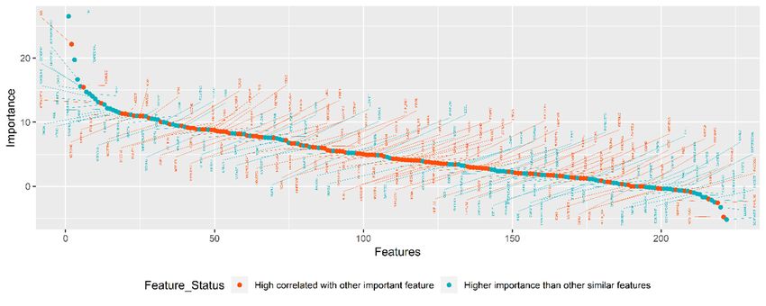
In the second step of TSFFS algorithm, the correlation and random forest feature importance
were used to choose the most relevant variable from similar variables. As shown in Figure 4, selected
variables are denoted by cyan points. The 116 variables were dropped because they have lower
importance than other similar variables. In other words, those variables have similar characteristics to
the remaining 106 variables. For example, the correlation between total value of financial assets (FIN)
and total value of assets (ASSET) is equal to 0.8287, but random forest importance of FIN and ASSET
are 10.40 and 4.13, respectively. In this case FIN is chosen because this variable is more important for
explaining borrowers’ creditworthiness.variables
were usedare denoted
to choose theby cyan
most points.variable
relevant The 116 variables
from similarwere dropped
variables. because
As shown they have
in Figure lower
4, selected
importance than other similar variables. In other words, those variables have
variables are denoted by cyan points. The 116 variables were dropped because they have lower similar characteristics
to the remaining
importance 106 variables.
than other For example,
similar variables. the words,
In other correlation
thosebetween
variablestotal
have value of financial
similar assets
characteristics
(FIN)
to the and total value
remaining of assets (ASSET)
106 variables. is equal
For example, thetocorrelation
0.8287, butbetween
random total
forestvalue
importance of FIN
of financial and
assets
ASSET are
Sustainability 10.40
2019, 11, and
699 4.13, respectively. In this case FIN is chosen because
(FIN) and total value of assets (ASSET) is equal to 0.8287, but random forest importance of FIN andthis variable is14more
of 23
important
ASSET arefor explaining
10.40 and 4.13, borrowers’ creditworthiness.
respectively. In this case FIN is chosen because this variable is more
Accordingly, the 106 variables were
important for explaining borrowers’ creditworthiness. retained to train the machine-learning model. Those
Accordingly, the 106 variables were retained to train the machine-learning model. Those variables
variables
Accordingly, the 106 variables were retainedthat
match with the part of the information to FICO credit
train the score requires tomodel.
machine-learning evaluate the
Those
match with the part of the information that FICO credit score requires to evaluate the borrower’s credit
borrower’s
variables creditwith
match scorethe
such as types
part of theofinformation
credit, payment history,
that FICO amounts
credit scoreowed, etc. to evaluate the
requires
score such as types of credit, payment history, amounts owed, etc.
borrower’s credit score such as types of credit, payment history, amounts owed, etc.
Figure 4. The result of feature selection using RF feature importance and correlation.
Figure 4. The result of feature selection using RF feature importance and correlation.
Figure 4. The result of feature selection using RF feature importance and correlation.
Finally, we
Finally, we assessed
assessed multicollinearity
multicollinearity onon the
the selected
selected variables
variables using
using VIF
VIF based
based on
on the
the logistic
logistic
regression.
regression. VIF
Finally,VIF is
we is a measure
assessed
a measure of the independent
multicollinearity variable’s
on thevariable’s
of the independent collinearity
selected variables using
collinearity with
withVIFthe
the other
based
otheronindependent
the logistic
independent
variables
regression. in the
VIF model.
is a In
measurethe literature,
of the when VIF
independent values
variable’sare less than 5
collinearity or 10
with values,
the multicollinearity
other
variables in the model. In the literature, when VIF values are less than 5 or 10 values, multicollinearity independent
is not
not an
an issue
variables
is issue inmodel.
in thein the regression
the regression model [81].
In the literature,
model [81].
whenFigure 55 shows
shows
VIF values
Figure the
arethe result
less of
thanof
result VIF
5 or
VIF for
10for each multicollinearity
values,
each selected variable
selected variable
and according
is notaccording
and an issue into this,
to the there is
this,regression no multicollinearity
there is nomodel in the
[81]. Figure 5inshows
multicollinearity model.
the result of VIF for each selected variable
the model.
and according to this, there is no multicollinearity in the model.
6
VIF for each variable Threshold = 5
6
(VIF)(VIF)
5 VIF for each variable Threshold = 5
5
factorfactor
4
inflation
4
3
inflation
3
The variance
2
The variance
2
1
1
0
THRIFT
KGTOTAL KGTOTAL
WAGEINC WAGEINC
EQUITINC EQUITINC
REFIN_EVERREFIN_EVER
FIN
TPAY
LEVRATIO LEVRATIO
MMDA
NBUSVEH NBUSVEH
BNKRUPLAST5
SAVING
REVPAY
LOCPAY
SAVRES6 SAVRES6
NEWCAR2 NEWCAR2
PURCH1
IFINPLAN IFINPLAN
WHYNOCKGWHYNOCKG
EOPAY
NOFINRISK NOFINRISK
SAVRES3 SAVRES3
SAVED
SAVRES1 SAVRES1
BFRIENDWORK
PAYVEH4 PAYVEH4
FUTPEN
PIR40
MORTBND MORTBND
OBND
CANTMANGCANTMANG
HHSEX
SVCCHG SVCCHG
BMAILADTVBMAILADTV
NONACTBUS
NSTOCKS NSTOCKS
COMUTF COMUTF
STMUTF
TFBMUTF TFBMUTF
IMAGZNEWS
HCDS
OBMUTF OBMUTF
MMMF
ISELF
SAVRES5 SAVRES5
IFRIENDWORK
GBMUTF GBMUTF
KIDS
FEARDENIAL
CASHLI
AGE
EDN_INST EDN_INST
ORESRE
INSTALL INSTALL
VLEASE
NNRESRE NNRESRE
EDCL
KGHOUSE KGHOUSE
BINTERNETBINTERNET
ANNUIT
MINBAL
BUSSEFARMINC
VEHIC
KGINC
EDUNUM EDUNUM
IDONT
DONTWANTDONTWANT
RACE
DBPLANCJ DBPLANCJ
CKPERSONAL
HCALL
ISHOPNONEISHOPNONE
HASSET
CKOTHCHOOSE
DONTLIKE DONTLIKE
DONTWRIT DONTWRIT
OTHER
CONSPAY CONSPAY
OTHNFIN OTHNFIN
SAVBND SAVBND
CHECKING CHECKING
LLOAN1
LLOAN6
OCCAT1
LLOAN5
LLOAN2
LLOAN8
ILNPAY
NTRAD
LLOAN11 LLOAN11
LLOAN4
PAYILN4 PAYILN4
BFINPLAN BFINPLAN
LLOAN7
MORT2
PAYMORTOPAYMORTO
NOTXBND NOTXBND
EHCHKG EHCHKG
TRANSFOTHINC
TURNDOWNTURNDOWN
GOVTBND GOVTBND
BFINPRO BFINPRO
IFINPRO
LLOAN9
TRUSTS
CKMANYSVCS
0
THRIFT
FIN
TPAY
MMDA
BNKRUPLAST5
SAVING
REVPAY
LOCPAY
PURCH1
EOPAY
SAVED
BFRIENDWORK
FUTPEN
PIR40
OBND
HHSEX
NONACTBUS
STMUTF
IMAGZNEWS
HCDS
MMMF
ISELF
IFRIENDWORK
KIDS
FEARDENIAL
CASHLI
AGE
ORESRE
VLEASE
EDCL
ANNUIT
MINBAL
IDONT
RACE
HASSET
CKOTHCHOOSE
BUSSEFARMINC
VEHIC
KGINC
CKPERSONAL
HCALL
TRANSFOTHINC
OTHER
LLOAN1
LLOAN6
OCCAT1
LLOAN5
LLOAN2
LLOAN8
ILNPAY
NTRAD
LLOAN4
LLOAN7
MORT2
IFINPRO
LLOAN9
TRUSTS
CKMANYSVCS
Selected Variables
Selected Variables
Figure 5. The variance inflation factor for selected variables.
Figure 5. The variance inflation factor for selected variables.
3.2.2. NAP Algorithm Figure 5. The variance inflation factor for selected variables.
Regarding NAP feature selection, since the SCF dataset consists of a large number of variables,
each variable was permuted 10 times to measure random forest importance. Then the p-value adjusted
by Bonferroni-Adjustment was assessed and the variables that had a p-value of less than 0.05 were
chosen. The NAP method assesses the null hypothesis that needs to be answered as: "Which variables
are related to other independent variables or to the dependent variable?" Accordingly, selected variables
provide two abilities: a higher predictive strength and being uncorrelated with some other variables.
The 76 variables were selected by NAP algorithm and the selected variables by TSFFS and NAP are
demonstrated in Tables S1 and S2 in the Supplementary Material.You can also read