Panoptic Segmentation Forecasting
←
→
Page content transcription
If your browser does not render page correctly, please read the page content below
Panoptic Segmentation Forecasting
*
Colin Graber1 Grace Tsai2 Michael Firman2 Gabriel Brostow2,3 Alexander Schwing1
1 2
University of Illinois at Urbana-Champaign Niantic 3 University College London
Abstract
arXiv:2104.03962v1 [cs.CV] 8 Apr 2021
Our goal is to forecast the near future given a set of re-
cent observations. We think this ability to forecast, i.e., to
anticipate, is integral for the success of autonomous agents
which need not only passively analyze an observation but
also must react to it in real-time. Importantly, accurate
forecasting hinges upon the chosen scene decomposition.
We think that superior forecasting can be achieved by de-
Input Frames
composing a dynamic scene into individual ‘things’ and
background ‘stuff’. Background ‘stuff’ largely moves be-
cause of camera motion, while foreground ‘things’ move
because of both camera and individual object motion. Fol-
lowing this decomposition, we introduce panoptic segmen-
tation forecasting. Panoptic segmentation forecasting opens
up a middle-ground between existing extremes, which either
forecast instance trajectories or predict the appearance of
future image frames. To address this task we develop a two-
component model: one component learns the dynamics of Our Panoptic Segmentation Forecast
the background stuff by anticipating odometry, the other one
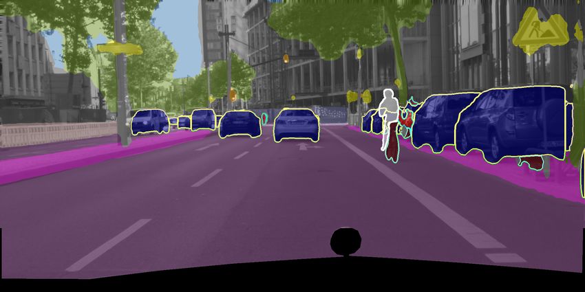
anticipates the dynamics of detected things. We establish a Figure 1. We study the novel task of ‘panoptic segmentation fore-
leaderboard for this novel task, and validate a state-of-the- casting’ and propose a state-of-the-art method that models the
art model that outperforms available baselines. motion of individual ‘thing’ instances separately while modeling
‘stuff’ as purely a function of estimated camera motion.
1. Introduction however, remains open: what is a suitable ‘state’ represen-
An intelligent agent must anticipate the outcome of its tation for the future of an observed scene?
movement in order to navigate safely [14, 41]. Said dif- Panoptic segmentation recently emerged as a rich repre-
ferently, successful autonomous agents need to understand sentation of a scene. Panoptic segmentation classifies each
the dynamics of their observations and forecast likely future pixel as either belonging to a foreground instance, the union
scenarios in order to successfully operate in an evolving en- of which is referred to as ‘things,’ or as a background class,
vironment. However, contemporary work in computer vi- referred to as ‘stuff’ [23, 5]. This decomposition is useful
sion largely analyzes observations, i.e., it studies the appar- for forecasting because we expect different dynamics for
ent. For instance, classical semantic segmentation [8, 42] each component: ‘stuff’ moves because of the observer’s
aims to delineate the observed outline of objects. While un- motion, while ‘things’ move because of both observer and
derstanding an observation is a first seminal step, it is only object motion. Use of panoptic segmentation is further un-
part of our job. Analyzing the currently observed frame derlined by the fact that it separates different instances of
means information is out of date by the time we know the objects, each of which we expect to move individually.
outcome, regardless of the processing time. It is even more Consequently, we propose to study the novel task of
stale by the time an autonomous agent can perform an ac- ‘panoptic segmentation forecasting’: given a set of ob-
tion. Successful agents therefore need to anticipate the fu- served frames, the goal is to forecast the panoptic segmen-
ture ‘state’ of the observed scene. An important question, tation for a set of unobserved frames (Fig. 1). We also pro-
pose a first approach to forecasting future panoptic segmen-
* Work done during an internship at Niantic. tations. In contrast to typical semantic forecasting [44, 52],
we model the motion of individual object instances and the        2.2. Methods That Anticipate
background separately. This makes instance information
                                                                      Anticipating, or synonymously ‘forecasting,’ has re-
persistent during forecasting, and allows us to understand
                                                                  ceived a considerable amount of attention in different com-
the motion of each moving object.
                                                                  munities [61]. Below, we briefly discuss work on forecast-
    To the best of our knowledge, we are the first to fore-       ing non-semantic information such as object location before
cast panoptic segmentations for future, unseen frames in          discussing forecasting of semantics and instances.
an image sequence. We establish a leaderboard for this            Forecasting of non-semantic targets: The most common
task on the challenging Cityscapes dataset [12] and in-           forecasting techniques operate on trajectories. They track
clude a set of baseline algorithms. Our method for fu-            and anticipate the future position of individual objects, ei-
ture panoptic segmentation relies on a number of innova-          ther in 2D or 3D [15, 46, 16, 71]. For instance, Hsieh et
tions (Sec. 3.1), that we ablate to prove their value. Our        al. [26] disentangle position and pose of multiple moving
method also results in state-of-the-art on previously es-         objects – but only on synthetic data. Like ours, Kosiorek et
tablished tasks of future semantic and instance segmen-           al. [34] track instances to forecast their future, but only in
tation. Code implementing models and experiments can              limited experimental scenarios.
be found at https://github.com/nianticlabs/                           Several methods forecast future RGB frames [38, 17,
panoptic-forecasting.                                             70]. Due to the high-dimensional space of the forecasts
                                                                  and due to ambiguity, results can be blurry, despite sig-
2. Related Work                                                   nificant recent advances. Uncertainty over future frames
                                                                  can be modelled, e.g., using latent variables [63, 70]. Re-
   We briefly review work which analyzes a single, given          lated to our approach, Wu et al. [66] treat foreground and
frame. We then discuss work which anticipates info about          background separately for RGB forecasting, but they do not
future, unseen frames. To reduce ambiguity, we avoid use of       model egomotion. All these methods differ from ours in
the word ‘predict,’ instead using analyze (looking at a cur-      output and architecture.
rent image) or anticipate (hypothesizing for a future frame).     Forecasting semantics: Recently, various methods have
                                                                  been proposed to estimate semantics for future, unobserved
2.1. Methods That Analyze                                         frames. Luc et al. [44] use a conv net to estimate the future
                                                                  semantics given as input the current RGB and semantics,
Semantic segmentation: Semantic segmentation has re-              while Nabavi et al. [48] use recurrent models with semantic
ceived a considerable amount of attention over decades.           maps as input. Chiu et al. [10] further use a teacher net to
The task requires methods to delineate the outline of ob-         provide the supervision signal during training, while Šarić
jects in a given image, either per instance or per object class   et al. [52] use learnable deformations to help forecast future
[56, 54, 57]. Recently, deep-net-based methods report state-      semantics from input RGB frames. However, these methods
of-the-art results [42, 1, 40]. Many architecture improve-        do not explicitly consider dynamics of the scene.
ments like dilated convolutions [72], skip-connections [51],          While Jin et al. [28] jointly predict flow and future se-
etc., have been developed for semantic segmentation before        mantics, some works explicitly warp deep features for fu-
they found use in other tasks. Our work differs as we care        ture semantic segmentation [53]. Similarly, Terwilliger et
about panoptic segmentation, and we aim to anticipate the         al. [59] use an LSTM to estimate a flow field to warp the
segmentation of future, unseen frames.                            semantic output from an input frame. However, by warping
Panoptic segmentation: Recently, panoptic segmenta-               in output space – rather than feature space – their model is
tion [32, 29] has emerged as a generalization of both se-         limited in its ability to reason about occlusions and depth.
mantic and instance segmentation. It requires methods to          While flow improves the modeling of the dynamic world,
give both a per-pixel semantic segmentation of an input im-       these methods only consider the dynamics at the pixel-level.
age while also grouping pixels corresponding to each object       Instead, we model dynamics at the object level.
instance. This ‘things’ vs. ‘stuff’ view of the world [23]            Recent methods [50, 62, 69, 25] estimate future frames
comes with its own set of metrics. Performing both tasks          by reasoning about shape, egomotion, and foreground mo-
jointly has the benefit of reducing computation [32, 68] and      tion separately. However, none of these methods reason ex-
enables both tasks to help each other [35, 37]. This is sim-      plicitly about individual instances, while our method yields
ilar in spirit to multi-task learning [33, 55]. Other works       a full future panoptic segmentation forecast.
have relaxed the high labeling demands of panoptic seg-           Forecasting future instances: Recent approaches for fore-
mentation [36] or improved architectures [49, 9]. Panoptic        casting instance segmentation use a conv net to regress the
segmentation has been extended to videos [30], but, again         deep features corresponding to the future instance segmen-
in contrast to our work only analyzing frames available at        tation [43] or LSTMs [58]. Couprie et al. [13] use a conv
test time without anticipating future results.                    net to forecast future instance contours together with an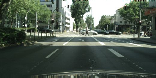
'Things' Forecasting (3.2.1)         Aggregation (3.2.3)

   Odometry Anticipation                                                             'Stuff' Forecasting
         (3.2.4)                                                                             (3.2.2)

Figure 2. Method overview. Given input frames I1,...,T , our method anticipates the panoptic segmentation ST +F of unseen frame IT +F .
Our method decomposes the scene into ‘things’ and ‘stuff’ forecasting. ‘Things’ are found via instance segmentation/tracking on the input
frames, after which we forecast the segmentation mask and depth of each individual instance (Sec. 3.1.1). Next, ‘Stuff’ is modeled by
warping input frame semantics to frame T + F using a 3d rigid-body transformation and then passing the result through a refinement
model (Sec. 3.1.2). Finally, we aggregate the forecasts from ‘things’ and ‘stuff’ into the final panoptic segmentation ST +F (Sec. 3.1.3).
Various components require future odometry obT +1,...,T +F , which we anticipate using input odometry o1,...,T (Sec. 3.1.4).

instance-wise semantic segmentation to estimate future in-              tected ‘things’ and one for the rest of the ‘stuff.’
stance segmentation. Their method only estimates fore-                      In addition to RGB images, we assume access to cam-
ground and not background semantics. Several works have                 era poses o1 , . . . , oT and depth maps d1 , . . . , dT for input
focused on anticipating future pose and location of specific            frames. Camera poses can come from odometry sensors or
object types, often people [45, 20]. Ye et al. [70] forecast fu-        estimates of off-the-shelf visual SLAM methods [6]. We
ture RGB frames by modeling each foreground object sepa-                obtained our depth maps from input stereo pairs [21] (these
rately. Unlike these works, we anticipate both instance seg-            could also be estimated from single frames [64]).
mentation masks for foreground objects and background se-                   An overview of our panoptic segmentation forecasting is
mantics for future time steps.                                          shown in Fig. 2. The method consists of four stages:
                                                                        1) ‘Things’ forecasting (Sec. 3.1.1): For each instance i,
3. Panoptic Segmentation Forecasting                                    we extract foreground instance tracks li from the observed
                                                                        input images I1 , . . . , IT . We use these tracks in our model
   We introduce Panoptic Segmentation Forecasting, a new
                                                                        to anticipate a segmentation mask m      b iT +F and depth dbiT +F
task which requires to anticipate the panoptic segmenta-
                                                                        for the unobserved future frame at time T + F .
tion for a future, unobserved scene. Different from clas-
sical panoptic segmentation which analyzes an observation,              2) ‘Stuff’ forecasting (Sec. 3.1.2): We predict the change
panoptic segmentation forecasting asks to anticipate what               in the background scene as a function of the anticipated
the panoptic segmentation looks like at a later time.                   camera motion, producing a background semantic output
                                                                        mbBT +F for the unobserved future frame IT +F .
   Formally, given a series of T RGB images I1 , . . . , IT of
height H and width W , the task is to anticipate the panoptic           3) Aggregation (Sec. 3.1.3): We aggregate foreground
segmentation ST +F that corresponds to an unobserved fu-                ‘things’ instance forecasts m    b iT +F and background scene
                                                                                    B
ture frame IT +F at a fixed number of timesteps F from the              forecast mb T +F , producing the final panoptic segmentation
last observation recorded at time T . Each pixel in ST +F is            output ST +F for future frame IT +F .
assigned a class c ∈ {1, . . . , C} and an instance ID.                 4) Odometry anticipation (Sec. 3.1.4): To better handle
                                                                        situations where we do not know future odometry, we train
3.1. Method                                                             a model to forecast odometry from the input motion history.
    Anticipating the state of a future unobserved scene                 3.1.1 ‘Things’ forecasting: The foreground prediction
requires to understand the dynamics of its components.                  model, sketched in Fig. 3, first locates the instance locations
‘Things’ like cars, pedestrians, etc. often traverse the world          li within the input sequence. These tracks are each then in-
‘on their own.’ Meanwhile, stationary ‘stuff’ changes po-               dependently processed by an encoder which captures their
sition in the image due to movement of the observer cam-                motion and appearance history. Encoder outputs are then
era. Because of this distinction, we expect the dynamics of             used to initialize the decoder, which predicts the appearance
‘things’ and ‘stuff’ to differ. Therefore, we develop a model           and location of instances for future frames, including depth
comprised of two components, one for the dynamics of de-                dbiT +F . These are processed using a mask prediction model
Detection and Tracking     Encoder                                       Decoder
Figure 3. The ‘Things’ forecasting model. This produces instance masks m     b iT +F for each instance i at target frame T + F . These masks
are obtained from input images I1 , . . . , IT via the following procedure: images are used to produce bounding box feature xit and mask
features rit using MaskR-CNN and DeepSort (left). These features are then input into an encoder to capture the instance motion history
(middle). Encoder outputs are used to initialize a decoder, which predicts the features x   biT +F and briT +F for target frame T + F (right).
These features are passed through a mask prediction head to produce the final output m  b iT +F . Here, T = 3 and T + F = 6.

                                   b iT +F .
to produce the final instance mask m                                      F steps until reaching the target time step T + F . More
   The output of the foreground prediction model is a set of              formally,
estimated binary segmentation masks m  b iT +F ∈ {0, 1}H×W
representing the per-pixel location for every detected in-                    hib,t = GRUdec ([b                   rit−1 )], hib,t−1 ),
                                                                                               xt−1 , ot , fmfeat (b                               (3)
stance i at frame T + F . Formally we obtain the mask via                       bit
                                                                                x     =   bit−1
                                                                                          x     + fbbox (hib,t ),                                  (4)
                                                                             him,t    =   ConvLSTMdec ([b   rit−1 , fbfeat (hib,t )], him,t−1 ),   (5)
        m̃iT +F = MaskOut b
                          riT +F ,

                                                                (1)

                                          i
                                                                              rit
                                                                                b     =   fmask (him,t ),                                          (6)
        b iT +F = Round Resize m̃iT +F , b
        m                                xT +F    .             (2)
                                                                          for t ∈ {T +1, . . . , T +F }, where ot represents the odome-
Here, in a first step, MaskOut uses a small convolutional                 try at time t, fbbox and fbfeat are multilayer perceptrons, and
network (with the same architecture as the mask decoder                   fmask and fmfeat are 1 × 1 convolutional layers.
of [22]) to obtain fixed-size segmentation mask probabil-                 Encoder. The decoder uses bounding box hidden state hib,T ,
ities m̃iT +F ∈ [0, 1]28×28 from a mask feature tensor                    appearance feature hidden state him,T , and estimates of the
riT +F ∈ R256×14×14 . In a second step, Resize scales
b                                                                         bounding box features b
                                                                                                     i
                                                                                                    xT and mask appearance features brT
                                                                                                                                        i
this mask to the size of the predicted bounding box rep-                  for the most recently observed frame IT . We obtain these
                                                         i
resented by the bounding box representation vector b   xT +F              quantities from an encoder which processes the motion and
using bilinear interpolation while filling all remaining lo-              appearance history of instance i. Provided with bounding
cations with 0. The bounding box information vector                       box features xit , mask features rit , and odometry ot for in-
  i
xT +F := [cx, cy, w, h, d, ∆cx, ∆cy, ∆w, ∆h, ∆d] con-
b                                                                         put time steps t ∈ {1, . . . , T }, the encoder computes the
tains object center coordinates, width, and height, which are             aforementioned quantities via
used in Resize, and also an estimate of the object’s distance
from the camera, and the changes of these quantities from                     hib,t = GRUenc ([xit−1 , ot−1 , fmfeat (rit−1 )], hib,t−1 ),         (7)
the previous frame, which will be useful later. The output
                                                                             him,t    =   ConvLSTMenc ([rit−1 , fbfeat (hib,t )], him,t−1 ).       (8)
depth dbiT +F is also obtained from this vector.
Decoder. To anticipate the bounding box information vec-                  Intuitively, the bounding box encoder is a GRU which pro-
      i
tor bxT +F and its appearance b riT +F , we use a decoder, as             cesses input bounding box features xit , odometry ot , and
shown on the right-hand-side of Fig. 3. It is comprised pri-              a transformation of mask features rit to produce box state
marily of two recurrent networks: a GRU [11] which mod-                   representation hib,T . Additionally, the mask appearance en-
els future bounding boxes and a ConvLSTM [67] which                       coder is a ConvLSTM which processes input mask features
models the future mask features. Intuitively, the GRU and                 rit and the representation of the input bounding box features
ConvLSTM update hidden states hib,t and him,t , represent-                hib,t produced by the bounding box encoder to obtain mask
ing the current location and appearance of instance i, as a               state representation him,T .
function of the bounding box features x   bt−1 and mask fea-                  The estimated mask and bounding box feature estimates
tures b rit−1 from the previous time step. These states are               for the final input time step T are computed by processing
used to predict location and appearance features for the cur-             the final encoder hidden states via
rent timestep, which are then autoregressively fed into the
model to forecast into the future; this process continues for                         biT = fenc,b (hib,T ), and b
                                                                                      x                          riT = fenc,m (him,T ),            (9)
where fenc,b is a multilayer perceptron and fenc,m is a 1 × 1           pixel correspondences between input frame t and target
convolution. These estimates are necessary because occlu-               frame T + F . After running a pre-trained semantic seg-
sions can prevent access to location and appearance for time            mentation model on frame It to get semantic segmentation
step T for some object instances. In those cases, use of                mt , we use these correspondences to map the semantic la-
Eq. (9) is able to fill the void.                                       bels from mt , which correspond to “stuff” classes, to pixels
Tracking. The encoder operates on estimated instance                    in frame T + F and maintain their projected depth at this
tracks/locations li := {ci , (xit , rit )|Tt=1 } which consist of ob-   frame. We denote the projected semantic map as m̃B      t and
ject class ci , bounding box features xit and mask features             the projected depth as d˜Bt .  However,  due  to 1) sparsity of
rit for all instances in the input video sequence I1 , . . . , IT .     the point clouds, and 2) lack of information in regions which
Obtaining these involves two steps: 1) we run MaskR-                    were previously occluded by foreground objects or were not
CNN [22] on every input frame to find the instances; 2) we              previously in-frame, only a subset of pixels in m̃B  t are as-
link instances across time using DeepSort [65]. For a given             signed a label. Therefore, we apply a refinement model that
                                                                        takes in (m̃B   ˜B
tracked instance i, we use outputs provided by MaskR-                               t , dt ) from all input frames to complete the se-
CNN, including predicted class ci , bounding boxes xit , and            mantic segmentation map m    bBT +F .
mask features rit extracted after the ROIAlign stage. The               Losses. To train the background refinement model, we use
distance d within xit refers to the median value of the input           a cross-entropy loss applied at pixels which do not corre-
depth map dt at locations corresponding to the estimated                spond to foreground objects in the target frame. This en-
instance segmentation mask found by MaskR-CNN for in-                   courages the output of the refinement network to match the
stance i in input frame t. A given object instance may not              ground truth semantic segmentation at each pixel. We for-
be found in all input frames, either due to the presence of             malize this in appendix Sec. E.2.
occlusions or because it has entered or left the scene. In
these cases, we set the inputs to an all zeros tensor.                  3.1.3 Aggregation: This step combines foreground in-
    Note that it is possible for instances to be missed during          stance segmentations m b iT +F , classes ci , depths diT +F and
the detection phase. We largely observe this to happen for              background semantic prediction m    bBT +F into the final future

static objects such as groups of bicycles parked on a side-             panoptic segmentation ST +F . For simplicity, we assume
walk (for instance, the right side of our prediction in the             that all foreground objects are located in front of all back-
fourth row of Fig. 4). One solution is to consider these in-            ground components. We found this to be valid in most
stances as part of the background forecasting. However, in              cases. Thus, to combine the foreground and background,
our experiments, we found that treating all the missed in-              we ‘paste’ foreground instances in order of decreasing pre-
stances as background degraded our performance because                  dicted instance depth on top of the background. This ap-
some instances are actually dynamic. Thus, in this paper,               proach is presented visually in Fig. 2, right, and described
we choose not to recover these instances.                               in more detail by Alg. 1 in the appendix.
Losses. To train the foreground model, we provide input                 3.1.4 Egomotion estimation: A large contributor to the
location and appearance features, predict their future states,          observed motion of a scene is the movement of the record-
and regress against their pseudo-ground-truth future states.            ing camera. Properly modeling this movement is critical
More specifically, the losses are computed using the esti-              for accurate results. Here, we consider two scenarios: 1) an
mated bounding boxes xit and instance features rit found by             ‘active’ scenario where the model has access to the planned
running instance detection and tracking on future frames.               motion of an autonomous agent; 2) a ‘passive’ scenario in
Note that losses are computed on intermediate predictions               which the camera is controlled by an external agent and
as well, which permits to properly model motion and ap-                 hence the model is not provided with the future motion.
pearance of instances across all future time steps. Our fore-              In the active scenario, we use the speed and yaw rate
ground model loss is a weighted sum of mean squared error               of the camera from the dataset, which we process into the
and L1 losses. See appendix Sec. E.1 for full details.                  forms required by the foreground and background models.
3.1.2 ‘Stuff’ forecasting: The background ‘stuff’ fore-                 See appendix Sec. B for more details.
                                                        bB                 In the passive scenario, we use a GRU to predict the
casting is tasked with predicting a semantic output m     T +F ∈
{1, . . . , Cstuff }H×W
                        for every pixel in the target frame T +         future camera motion as a function of its past movement.
F . We assume they correspond to the static part of the                 More formally and as sketched in Fig. 2(left),
scene, i.e., background changes in the images are caused                 ho,t+1 = GRUcam (b
                                                                                          ot , ho,t ) and obt+1 = fcam (ho,t+1 ), (10)
solely by camera motion.
   We predict the background changes by back-projecting                 where fcam is a multilayer perceptron. For input time steps,
3D points from the background pixels in frame t given depth             i.e., t ∈ {1, . . . , T }, we use known camera motion ot as
dt and camera intrinsics, transforming with ego-motion ot ,             model input. For future time steps, i.e., t ∈ {T +1, . . . , T +
and projecting to frame T + F . This process establishes                F }, we use predicted camera motion obt as input.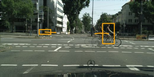
Short term: ∆t = 3                                               Mid term: ∆t = 9
                                             All                    Things                Stuff                 All                Things                  Stuff
                                      PQ     SQ       RQ     PQ       SQ    RQ    PQ       SQ     RQ     PQ     SQ     RQ     PQ     SQ     RQ       PQ     SQ     RQ
 Panoptic Deeplab (Oracle)†           60.3   81.5     72.9   51.1   80.5   63.5   67.0    82.3    79.7   60.3   81.5   72.9   51.1   80.5   63.5    67.0   82.3    79.7
 Panoptic Deeplab (Last seen frame)   32.7   71.3     42.7   22.1   68.4   30.8   40.4    73.3    51.4   22.4   68.5   30.4   10.7   65.1   16.0    31.0   71.0    40.9
 Flow                                 41.4   73.4     53.4   30.6   70.6   42.0   49.3    75.4    61.8   25.9   69.5   34.6   13.4   67.1   19.3    35.0   71.3    45.7
 Hybrid [59] (bg) and [43] (fg)       43.2   74.1     55.1   35.9   72.4   48.3   48.5    75.3    60.1   29.7   69.1   39.4   19.7   66.8   28.0    37.0   70.8    47.7
 Ours                                 49.0   74.9     63.3   40.1   72.5   54.6   55.5    76.7    69.5   36.3   71.3   47.8   25.9   69.0   36.2    43.9   72.9    56.2

Table 1. Panoptic segmentation forecasting evaluated on the Cityscapes validation set. † has access to the RGB frame at ∆t. Higher
is better for all metrics.
         Last Seen Image                            Oracle                         Flow                         Hybrid                             Ours

Figure 4. Mid-term panoptic segmentation forecasts on Cityscapes. Compared to Hybrid, our approach produces more well-defined
silhouettes for instance classes (see the cars in the 1st row or the pedestrians in the 4th row), and handles instances with large motion much
better Hybrid – the car in the 2nd row is not predicted to have moved sufficiently; the cyclist in the 3rd row is not predicted at all. Since
Flow does not model instance-level trajectory, the ‘things’ are no longer intact in the forecasts.

4. Evaluation                                                                              frame as input and evaluate two different scenarios: short-
                                                                                           term forecasting looks 3 frames (∼0.18s) and medium-term
   We establish the first results for the task of panoptic                                 forecasting looks 9 frames (∼0.53s) into the future. All
segmentation forecasting by comparing our developed ap-                                    metrics are computed on the 20th frame of the sequence.
proach to several baselines. We also provide ablations to                                  We use an input length of T = 3. We hence use frames 11,
demonstrate the importance of our modeling decisions. We                                   14, and 17 as input for short-term experiments and frames
additionally evaluate on the tasks of semantic segmentation                                5, 8, and 11 as input for medium-term experiments.
forecasting and instance segmentation forecasting to com-
pare our method to prior work on established tasks.                                        4.1. Panoptic Segmentation Forecasting
Data: To evaluate panoptic segmentation forecasting, we                                    Metrics. We compare all approaches using metrics intro-
need a dataset which contains both semantic and instance                                   duced in prior work [32] on panoptic segmentation. These
information as well as entire video sequences that lead up                                 metrics require to first compute matches between predicted
to the annotated frames. Cityscapes [12] fulfills these re-                                segments and ground truth segments. A match between a
quirements and has been used in prior work for semantic                                    predicted segment and a ground truth segment of the same
and instance forecasting. This dataset consists of 5000 se-                                class is a true positive if their intersection over union (IoU)
quences of 30 frames each, spanning approximately 1.8 sec-                                 is larger than 0.5. Using these matches, three metrics are
onds. The data were recorded from a car driving in urban                                   considered: segmentation quality (SQ), which is the average
scenarios, and semantic and instance annotations are pro-                                  IoU of true positive matched segments, recognition quality
vided for the 20th frame in each sequence. Following stan-                                 (RQ), which is the F1 score computed over matches, and
dard practice for prior work in forecasting segmentations                                  panoptic quality (PQ), which is the product of SQ and RQ.
[44, 43, 59, 53], all experiments presented here are run on                                All of these metrics are computed per class and then aver-
the validation data; a limited set of evaluations on test data                             aged to compute the final score.
are presented in appendix Sec. G.                                                          Baselines. To compare our approach against baselines on
   To match prior work [44, 43, 53], we use every third                                    the novel task of panoptic segmentation forecasting, we use:
∆t = 3               ∆t = 9                               Short term: ∆t = 3   Mid term: ∆t = 9
                                 PQ     SQ RQ        PQ      SQ RQ            Accuracy (mIoU)     All        MO       All       MO
Ours                            49.0   74.9   63.3   36.3   71.3   47.8       Oracle             80.6      81.7       80.6     81.7
1) w/ Hybrid bg [59]            45.0   74.1   57.9   32.4   70.1   42.9
                                                                              Copy last          59.1      55.0       42.4     33.4
2) w/ Hybrid fg [43]            47.3   74.8   60.7   33.4   70.4   43.9
                                                                              3Dconv-F2F [10]    57.0        /        40.8       /
3) w/ linear instance motion    40.2   73.7   52.1   27.9   70.1   36.6
                                                                              Dil10-S2S [44]     59.4      55.3       47.8     40.8
4) fg w/o odometry              48.8   75.1   62.8   35.3   71.1   46.5
                                                                              LSTM S2S [48]      60.1        /          /        /
5) w/ ORB-SLAM odometry         48.6   75.0   62.5   36.1   71.3   47.5
                                                                              Bayesian S2S [4]   65.1        /        51.2       /
6) w/ SGM depth                 48.8   75.2   62.8   36.1   71.4   47.3
                                                                              DeformF2F [52]     65.5      63.8       53.6     49.9
7) w/ monocular depth           47.5   74.8   61.0   34.8   70.9   45.8
                                                                              LSTM M2M [59]      67.1      65.1       51.5     46.3
w/ ground truth future odometry 49.4 75.2 63.5 39.4 72.1 51.6                 F2MF [53]          69.6      67.7       57.9     54.6
                                                                              Ours               67.6      60.8       58.1     52.1
Table 2. Validating our design choices using Cityscapes. Higher
is better for all metrics. All approaches use predicted future odom-      Table 3. Semantic forecasting results on the Cityscapes valida-
etry unless otherwise specified.                                          tion dataset. Baseline numbers, besides oracle and copy last, are
                                                                          from [53]. Higher is better for all metrics. Our model exploits
Panoptic Deeplab (Oracle): we apply the Panoptic Deeplab                  stereo and odometry, which are provided by typical autonomous
model [9] to analyze the target frame. This represents an                 vehicle setups and are included in Cityscapes.
upper bound on performance, as it has direct access to fu-
                                                                          tion replaces the foreground forecasting model with a sim-
ture information.
                                                                          ple model assuming linear instance motion and no mask ap-
Panoptic Deeplab (Last seen frame): we apply the same
                                                                          pearance change; 4) fg w/o odometry does not use odometry
Panoptic Deeplab model to the most recently observed
                                                                          as input to the foreground model; 5) w/ ORB-SLAM odome-
frame. This represents a model that assumes no camera or
                                                                          try uses input odometry obtained from [6]; 6) w/ SGM depth
instance motion.
                                                                          uses depths obtained from SGM [24] provided by [12] as in-
Flow: Warp the panoptic segmentation analyzed at the last
                                                                          put to the model; and 7) w/ monocular depth uses a monoc-
observed frame using optical flow [27] computed from the
                                                                          ular depth prediction model [19], finetuned on Cityscapes,
last two observed frames.
                                                                          to obtain input depth. Ablations 1) and 2) show that our
Hybrid Semantic/Instance Forecasting: We fuse predictions
                                                                          improved model performance is due to the strength of both
made by a semantic segmentation forecasting model [59]
                                                                          our foreground and background components. Ablation 3)
and an instance segmentation forecasting model [43] to cre-
                                                                          shows that joint modeling of instance motion and appear-
ate a panoptic segmentation for the target frame.
                                                                          ance mask is key to success. 4) shows that odometry inputs
Results. The results for all models on the panoptic seg-
                                                                          help the model predict foreground locations better, and 5)
mentation forecasting task are presented in Tab. 1. We out-
                                                                          demonstrates our method works well with odometry com-
perform all non-oracle approaches on the PQ, SQ, and RQ
                                                                          puted directly from input images. 6) and 7) suggest that our
metrics for both short-term and mid-term settings. The im-
                                                                          approach benefits from more accurate depth prediction, but
provements to PQ and RQ show that our model better cap-
                                                                          it also works well with depth inputs obtained using single-
tures the motion of all scene components, including static
                                                                          frame methods.
background ‘stuff’ regions and dynamic ‘things.’ In ad-
dition, the improvements to SQ imply that the per-pixel                   4.2. Semantic Segmentation Forecasting
quality of true positive matches are not degraded. The
Flow model performs worse than either Hybrid or our ap-                       For a comprehensive comparison, we also assess our ap-
proach, which demonstrates that a simple linear extrapola-                proach on the task of semantic segmentation forecasting.
tion of per-pixel input motion is not sufficient to capture the           This task asks to anticipate the correct semantic class per
scene and object movement. The fact that the gap between                  pixel for the target frame. Unlike the panoptic segmenta-
ours and Hybrid on ‘things’ PQ grows between the short-                   tion evaluation, this task doesn’t care about instances, i.e.,
and mid-term settings shows the strength of our foreground                good performance only depends on the ability to anticipate
model (Sec. 3.1.1) on anticipating object motion at longer                the correct semantic class for each pixel. We obtain seman-
time spans. Fig. 4 compares results to baselines. Our ap-                 tic segmentation outputs from our model by discarding in-
proach produces better defined object silhouettes and han-                stance information and only retaining the semantics.
dles large motion better than the baselines.                              Metrics. Future semantic segmentation is evaluated using
Ablations. Tab. 2 shows results for ablation experi-                      intersection over union (IoU) of predictions compared to the
ments which analyze the impact of our modeling choices:                   ground truth, which are computed per class and averaged
1) w/Hybrid bg uses our foreground model, but replaces our                over classes. We additionally present an IoU score which is
background model with the one from [59]; 2) w/Hybrid fg                   computed by averaging over ‘things’ classes only (MO).
uses our background model, but replaces our foreground                    Baselines. We compare to a number of recent works which
model with the one from [43]; 3) w/linear instance mo-                    forecast semantic segmentations. Many of these approaches
Short term: ∆t = 3   Mid term: ∆t = 9
                       AP        AP50      AP        AP50
    Oracle            34.6      57.4       34.6     57.4
    Last seen frame   8.9       21.3       1.7      6.6
    F2F [43]          19.4      39.9       7.7      19.4
    Ours              17.8      38.4       10.0     22.3         Figure 5. Failure cases. Left: the cyclist highlighted in white was
Table 4. Instance segmentation forecasting on the Cityscapes     missed by instance detection. Right: mispredicted odometry leads
validation dataset. Higher is better for all metrics.            to misalignment between the forecast and the target image (the
                                                                 outlines of objects in the target image are shown in white).
anticipate the features of a future scene [44, 48, 4, 52, 10,
53]. LSTM M2M [59] anticipates the optical flow between          4.4. Introspection
the most recent frame and the target with a warping func-            Why does our approach anticipate higher-fidelity in-
tion transforming input semantics. Different from these,         stances than prior approaches? Many of these works at-
we decompose the prediction into feature predictions for         tempt to predict future scenes by anticipating what a fixed-
each individual instance as well as a transformation of back-    size feature tensor for the entire image will look like – this is
ground semantics before combining. Additionally, these ap-       true for both semantic segmentation forecasting [44, 10, 53]
proaches do not use depth inputs and all except Bayesian         and instance segmentation forecasting [43]. Note, this con-
S2S [4] do not use egomotion as input.                           flates camera motion, which objects are present in a scene,
Results. The results for this task are given in Tab. 3. We       how these objects move, and how the appearance of ob-
outperform most models on standard IoU as well as MO             jects and background components change as a function of
IoU. Unlike all other baselines, our model is able to produce    the scene motion. This increases the complexity of the
instance-level predictions for moving object classes, which      prediction. Instead, our method decomposes these com-
is a more challenging objective.                                 ponents into individual parts: the foreground model an-
4.3. Instance Segmentation Forecasting                           ticipates how each object moves and how its appearance
                                                                 changes as a function of this motion; the background model
    We also evaluate on instance segmentation forecast-          captures how static scene components appear when the
ing, which only focuses on the ‘things’ classes within           camera moves; and the odometry model anticipates likely
Cityscapes. Future instance segmentation can be obtained         future motion based on past input. Modeling each of these
from our model by disregarding all pixels corresponding to       separately simplifies individual prediction. Additionally,
‘stuff’ classes from the panoptic forecasting output.            we predict separate features for every individual instance,
Metrics. Instance segmentation is evaluated using two met-       so its size scales with the number of instances present in a
rics [12]: 1) Average Precision (AP) first averages over a       scene, while past approaches [43] use a fixed size represen-
number of overlapping thresholds required for matches to         tation regardless of the complexity of the scene.
count as true positives and is then averaged across classes;         The performance of our approach is hampered in some
2) AP50 is the average precision computed using an overlap       cases by failures in instance detection and tracking (exam-
threshold of 0.5 which is then averaged across classes.          ples in Fig. 5). At the moment, our model cannot properly
Baselines. There is very little prior work on instance seg-      recover from situations where the input is noisy. That be-
mentation forecasting. We compare to Luc et al. [43], who        ing said, our approach immediately benefits from improve-
train a model to predict the features of the entire future       ments in the areas of instance detection and tracking, which
scene using a convolutional model and obtain final instances     are very active fields of research [2, 3].
by running these predicted features through the prediction
heads of MaskR-CNN. Instead, our approach predicts an in-        5. Conclusions
dividual set of features for each instance found in the scene.      We introduced the novel task ‘panoptic segmentation
Results. Tab. 4 presents the results. We outperform prior        forecasting.’ It requires to anticipate a per-pixel instance-
work in the mid-term setting. This indicates that model-         level segmentation of ‘stuff’ and ‘things’ for an unobserved
ing trajectory of individual instances has a higher potential    future frame given as input a sequence of past frames. To
on forecasting tasks. Since we use the same model cre-           solve this task, we developed a model which anticipates tra-
ated by Luc et al. [43] as the ‘foreground’ component of         jectory and appearance of ‘things’ and by reprojecting input
the Hybrid baseline (Sec. 4.1), Fig. 4 shows visual compar-      semantics for ‘stuff.’ We demonstrated that the method out-
isons between these approaches. Again, our method gives          performs compelling baselines on panoptic, semantic and
higher-detailed instance contours and models objects with        instance segmentation forecasting.
larger motion more accurately. Moreover, in some cases,          Acknowledgements: This work is supported in part by
F2F “deletes” some instances from the scene (such as the         NSF under Grant #1718221, 2008387, 2045586, MRI
cyclist in row 3).                                               #1725729, and NIFA award 2020-67021-32799.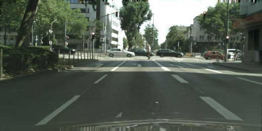
References                                                            [19] C. Godard, O. Mac Aodha, M. Firman, and G. J. Brostow.
                                                                          Digging into self-supervised monocular depth estimation. In
[1] V. Badrinarayanan, A. Kendall, and R. Cipolla. Segnet: A              ICCV, 2019.
    deep convolutional encoder-decoder architecture for image         [20] C. Graber and A. Schwing. Dynamic neural relational infer-
    segmentation. PAMI, 2017.                                             ence. In CVPR, 2020.
[2] P. Bergmann, T. Meinhardt, and L. Leal-Taixe. Tracking with-      [21] X. Gu, Z. Fan, S. Zhu, Z. Dai, F. Tan, and P. Tan. Cascade
    out bells and whistles. In ICCV, 2019.                                cost volume for high-resolution multi-view stereo and stereo
[3] G. Bertasius and L. Torresani. Classifying, segmenting, and           matching. In CVPR, 2020.
    tracking object instances in video with mask propagation. In      [22] K. He, G. Gkioxari, P. Dollár, and R. Girshick. Mask R-
    CVPR, 2020.                                                           CNN. In ICCV, 2017.
[4] A. Bhattacharyya, M. Fritz, and B. Schiele. Bayesian predic-      [23] G. Heitz and D. Koller. Learning spatial context: Using stuff
    tion of future street scenes using synthetic likelihoods. ICLR,       to find things. In ECCV, 2008.
    2019.                                                             [24] H. Hirschmuller. Accurate and efficient stereo processing
[5] H. Caesar, J. Uijlings, and V. Ferrari. Coco-stuff: Thing and         by semi-global matching and mutual information. In CVPR,
    stuff classes in context. In CVPR, 2018.                              2005.
[6] C. Campos, R. Elvira, J. J. Gómez, J. M. M. Montiel, and J. D.   [25] L. Hoyer, P. Kesper, A. Khoreva, and V. Fischer. Short-
    Tardós. ORB-SLAM3: An accurate open-source library for               term prediction and multi-camera fusion on semantic grids.
    visual, visual-inertial and multi-map SLAM. arXiv preprint            In ICCV Workshops, 2019.
    arXiv:2007.11898, 2020.                                           [26] J.-T. Hsieh, B. Liu, D.-A. Huang, L. Fei-Fei, and J. C.
                                                                          Niebles. Learning to decompose and disentangle represen-
[7] P. Chao, C.-Y. Kao, Y.-S. Ruan, C.-H. Huang, and Y.-L. Lin.
                                                                          tations for video prediction. In NeurIPS, 2018.
    Hardnet: A low memory traffic network. In ICCV, 2019.
                                                                      [27] E. Ilg, N. Mayer, T. Saikia, M. Keuper, A. Dosovitskiy, and
[8] L.-C. Chen, G. Papandreou, I. Kokkinos, K. Murphy, and                T. Brox. Flownet 2.0: Evolution of optical flow estimation
    A. L. Yuille. Semantic image segmentation with deep con-              with deep networks. In CVPR, 2017.
    volutional nets and fully connected CRFs. arXiv:1412.7062,        [28] X. Jin, H. Xiao, X. Shen, J. Yang, Z. Lin, Y. Chen, Z. Jie,
    2014.                                                                 J. Feng, and S. Yan. Predicting scene parsing and motion dy-
[9] B. Cheng, M. D. Collins, Y. Zhu, T. Liu, T. S. Huang,                 namics in the future. In NeurIPS, 2017.
    H. Adam, and L.-C. Chen. Panoptic-DeepLab: A simple,              [29] A. Kendall, Y. Gal, and R. Cipolla. Multi-task learning using
    strong, and fast baseline for bottom-up panoptic segmentation.        uncertainty to weigh losses for scene geometry and semantics.
    In CVPR, 2020.                                                        In CVPR, 2018.
[10] H.-K. Chiu, E. Adeli, and J. C. Niebles. Segmenting the          [30] D. Kim, S. Woo, J.-Y. Lee, and I. S. Kweon. Video panoptic
    future. IEEE Robotics and Automation Letters, 2020.                   segmentation. In CVPR, 2020.
[11] K. Cho, B. Van Merriënboer, C. Gulcehre, D. Bahdanau,           [31] D. Kingma and J. Ba. Adam: A method for stochastic opti-
    F. Bougares, H. Schwenk, and Y. Bengio. Learning phrase               mization. arXiv:1412.6980, 2014.
    representations using RNN encoder-decoder for statistical ma-     [32] A. Kirillov, K. He, R. Girshick, C. Rother, and P. Dollár.
    chine translation. arXiv:1406.1078, 2014.                             Panoptic segmentation. In CVPR, 2019.
[12] M. Cordts, M. Omran, S. Ramos, T. Rehfeld, M. Enzweiler,         [33] I. Kokkinos. Ubernet: Training a universal convolutional
    R. Benenson, U. Franke, S. Roth, and B. Schiele. The                  neural network for low-, mid-, and high-level vision using di-
    cityscapes dataset for semantic urban scene understanding. In         verse datasets and limited memory. In CVPR, 2017.
    CVPR, 2016.                                                       [34] A. Kosiorek, H. Kim, Y. W. Teh, and I. Posner. Sequential
[13] C. Couprie, P. Luc, and J. Verbeek. Joint future semantic and        attend, infer, repeat: Generative modelling of moving objects.
    instance segmentation prediction. In ECCV workshops, 2018.            In NeurIPS, 2018.
                                                                      [35] J. Li, A. Raventos, A. Bhargava, T. Tagawa, and A. Gaidon.
[14] K. J. W. Craik. The Nature of Explanation. Cambridge Uni-
                                                                          Learning to fuse things and stuff. arXiv:1812.01192, 2018.
    versity Press, 1943.
                                                                      [36] Q. Li, A. Arnab, and P. H. Torr. Weakly-and semi-supervised
[15] Q. Dai, V. Patil, S. Hecker, D. Dai, L. Van Gool, and                panoptic segmentation. In ECCV, 2018.
    K. Schindler. Self-supervised object motion and depth esti-
                                                                      [37] Y. Li, X. Chen, Z. Zhu, L. Xie, G. Huang, D. Du, and
    mation from video. In CVPR Workshops, 2020.
                                                                          X. Wang. Attention-guided unified network for panoptic seg-
[16] S. Ehrhardt, O. Groth, A. Monszpart, M. Engelcke, I. Pos-            mentation. In CVPR, 2019.
    ner, N. Mitra, and A. Vedaldi. RELATE: Physically plausible       [38] X. Liang, L. Lee, W. Dai, and E. P. Xing. Dual motion GAN
    multi-object scene synthesis using structured latent spaces. In       for future-flow embedded video prediction. In ICCV, 2017.
    NeurIPS, 2020.                                                    [39] T.-Y. Lin, M. Maire, S. Belongie, J. Hays, P. Perona, D. Ra-
[17] H. Gao, H. Xu, Q.-Z. Cai, R. Wang, F. Yu, and T. Darrell.            manan, P. Dollár, and C. L. Zitnick. Microsoft coco: Common
    Disentangling propagation and generation for video predic-            objects in context. In ECCV, 2014.
    tion. In ICCV, 2019.                                              [40] C. Liu, L.-C. Chen, F. Schroff, H. Adam, W. Hua, A. L.
[18] A. Geiger, P. Lenz, and R. Urtasun. Are we ready for Au-             Yuille, and L. Fei-Fei. Auto-deeplab: Hierarchical neural ar-
    tonomous Driving? The KITTI Vision Benchmark Suite. In                chitecture search for semantic image segmentation. In CVPR,
    CVPR, 2012.                                                           2019.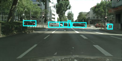
[41] R. R. Llinás. I of the vortex: from neurons to self. MIT Press,       [63] J. Walker, C. Doersch, A. Gupta, and M. Hebert. An uncer-
    2001.                                                                       tain future: Forecasting from static images using variational
[42] J. Long, E. Shelhamer, and T. Darrell. Fully convolutional                 autoencoders. In ECCV, 2016.
    networks for semantic segmentation. In CVPR, 2015.                      [64] J. Watson, M. Firman, G. Brostow, and D. Turmukhambetov.
[43] P. Luc, C. Couprie, Y. LeCun, and J. Verbeek. Predicting fu-               Self-supervised monocular depth hints. In ICCV, 2019.
    ture instance segmentation by forecasting convolutional fea-            [65] N. Wojke, A. Bewley, and D. Paulus. Simple online and real-
    tures. In ECCV, 2018.                                                       time tracking with a deep association metric. In ICIP, 2017.
[44] P. Luc, N. Neverova, C. Couprie, J. Verbeek, and Y. LeCun.             [66] Y. Wu, R. Gao, J. Park, and Q. Chen. Future video synthesis
    Predicting deeper into the future of semantic segmentation. In              with object motion prediction. In CVPR, 2020.
    ICCV, 2017.                                                             [67] S. Xingjian, Z. Chen, H. Wang, D.-Y. Yeung, W.-K. Wong,
[45] K. Mangalam, E. Adeli, K.-H. Lee, A. Gaidon, and J. C.                     and W.-c. Woo. Convolutional lstm network: A machine
    Niebles. Disentangling human dynamics for pedestrian loco-                  learning approach for precipitation nowcasting. In NIPS,
    motion forecasting with noisy supervision. In WACV, 2020.                   2015.
[46] J. Martinez, M. J. Black, and J. Romero. On human motion               [68] Y. Xiong, R. Liao, H. Zhao, R. Hu, M. Bai, E. Yumer, and
    prediction using recurrent neural networks. In CVPR, 2017.                  R. Urtasun. UPSNet: A unified panoptic segmentation net-
[47] A. Milan, L. Leal-Taixé, I. Reid, S. Roth, and K. Schindler.              work. In CVPR, 2019.
    Mot16: A benchmark for multi-object tracking. arXiv preprint
                                                                            [69] J. Xu, B. Ni, Z. Li, S. Cheng, and X. Yang. Structure pre-
    arXiv:1603.00831, 2016.
                                                                                serving video prediction. In CVPR, 2018.
[48] S. S. Nabavi, M. Rochan, and Y. Wang. Future semantic
                                                                            [70] Y. Ye, M. Singh, A. Gupta, and S. Tulsiani. Compositional
    segmentation with convolutional LSTM. In BMVC, 2018.
                                                                                video prediction. In ICCV, 2019.
[49] L. Porzi, S. Rota Bulò, A. Colovic, and P. Kontschieder.
                                                                            [71] R. Yeh, A. G. Schwing, J. Huang, and K. Murphy. Diverse
    Seamless scene segmentation. In CVPR, 2019.
                                                                                Generation for Multi-agent Sports Games. In Proc. CVPR,
[50] X. Qi, Z. Liu, Q. Chen, and J. Jia. 3D motion decomposition
                                                                                2019.
    for RGBD future dynamic scene synthesis. In CVPR, 2019.
[51] O. Ronneberger, P. Fischer, and T. Brox. U-net: Convo-                 [72] F. Yu and V. Koltun. Multi-scale context aggregation by di-
    lutional networks for biomedical image segmentation. In                     lated convolutions. arXiv:1511.07122, 2015.
    International Conference on Medical image computing and                 [73] Y. Zhu, K. Sapra, F. A. Reda, K. J. Shih, S. Newsam, A. Tao,
    computer-assisted intervention, 2015.                                       and B. Catanzaro. Improving semantic segmentation via video
[52] J. Šarić, M. Oršić, T. Antunović, S. Vražić, and S. Šegvić.       propagation and label relaxation. In CVPR, 2019.
    Single level feature-to-feature forecasting with deformable
    convolutions. In German Conference on Pattern Recognition,
    2019.
[53] J. Saric, M. Orsic, T. Antunovic, S. Vrazic, and S. Segvic.
    Warp to the future: Joint forecasting of features and feature
    motion. In CVPR, 2020.
[54] F. Schroff, A. Criminisi, and A. Zisserman. Object class seg-
    mentation using Random Forests. In BMVC, 2008.
[55] O. Sener and V. Koltun. Multi-task learning as multi-
    objective optimization. In NeurIPS, 2018.
[56] E. Sharon, A. Brandt, and R. Basri. Segmentation and
    boundary detection using multiscale intensity measurements.
    In CVPR, 2001.
[57] J. Shotton, M. Johnson, and R. Cipolla. Semantic texton
    forests for image categorization and segmentation. In CVPR,
    2008.
[58] J. Sun, J. Xie, J.-F. Hu, Z. Lin, J. Lai, W. Zeng, and W.-s.
    Zheng. Predicting future instance segmentation with contex-
    tual pyramid convLSTMs. In ACM International Conference
    on Multimedia, 2019.
[59] A. Terwilliger, G. Brazil, and X. Liu. Recurrent flow-guided
    semantic forecasting. In WACV, 2019.
[60] S. Thrun, W. Burgard, and D. Fox. Probabilistic robotics.
    MIT, 2005.
[61] E. Valassakis. Future object segmentation for complex cor-
    related motions. Master’s thesis, UCL, 2018.
[62] S. Vora, R. Mahjourian, S. Pirk, and A. Angelova. Future
    semantic segmentation using 3D structure. arXiv:1811.11358,
    2018.
Appendix: Panoptic Segmentation Forecasting
In this appendix, we first provide additional details on
the classes contained within Cityscapes (Sec. A). This is
followed by details deferred from the main paper for space
reasons, including a description of how odometry is used
by each component (Sec. B), formal descriptions of the
background modeling approach (Sec. C), the aggregation Figure 6. ‘Stuff’ forecasting is achieved in two steps. First, for
method (Sec. D), used losses (Sec. E), and miscellaneous each input frame t ∈ {1, . . . , T } given depth map dB t and ego-
implementation details for all model components and base- motion, project the semantic map mB t for all the background pix-
els on to frame T + F . Note the sparsity of the projected semantic
lines (Sec. F). This is followed by additional experimen-
maps. Second, we apply a refinement network to complete the
tal results (Sec. G), including per-class panoptic segmenta- background segmentation.
tion metrics as well as metrics computed on test data for
the tasks of panoptic, semantic, and instance segmentation
forecasting. Finally, we present additional visualizations of where (xt+1 , yt+1 ) is the location of the vehicle at time t+1
model predictions (Sec. H). treating the vehicle at time t as the origin (x-axis is front, y-
Included in the supplementary material are videos visu- axis is left, and z-axis is up), and θt is the rotation of the
alizing results and a few of the baselines. These are de- vehicle at time t along the z-axis. We then extend (x, y, θ)
scribed in more detail in Sec. H. into a 6-dof transform Htt+1 , and apply the camera extrin-
cam
sics Hveh to obtain the transform of the cameras from frame
A. ‘Things’ and ‘Stuff’ class breakdown in t to frame t + 1 via,
Cityscapes
cos θt − sin θt 0 xt+1
The data within Cityscapes are labeled using 19 seman- sin θt cos θt 0 yt+1
Hveh,t = 0
, (15)
tic classes. The ‘things’ classes are those that refer to in- 0 1 0
dividual objects which are potentially moving in the world 0 0 0 1
and consist of person, rider, car, truck, bus, train, motorcy- cam −1 cam −1
Htt+1 = Hveh Hveh,t (Hveh ) . (16)
cle, and bicycle. The remaining 11 classes are the ‘stuff’
classes and consist of road, sidewalk, building, wall, fence, The final transform HtT +F from frame t to frame T + F is
pole, traffic light, traffic sign, vegetation, terrain, and sky. obtained by concatenating the consecutive transforms Htt+1
for t ∈ {1, . . . , T + F − 1}.
B. Odometry For egomotion estimation (Sec. 3.1.4), ot is used as input
for frames t ∈ {1, . . . , T } and predicted for frames t ∈
Cityscapes provides vehicle odometry ot at each frame
{T + 1, . . . , T + F }. For ‘things’ forecasting (Sec. 3.1.1),
t as [vt , ∆θt ], where vt is the speed and ∆θt is the yaw
the input egomotion vector consists of vt , θt , xt+1 , yt+1 ,
rate. This odometry assumes the vehicle is moving on a
and θt+1 , i.e., the speed and yaw rate of the vehicle as well
flat ground plane with no altitude changes. For background
as how far the vehicle moves in this time step.
forecasting (Sec. 3.1.2), a full 6-dof transform Ht from
frame t and the target frame T +F is required for projecting
the 3d semantic point cloud (m̃B ˜B C. Detail on background modelling
t , dt ).
To derive Ht , we use the odometry readings o1,...,T +F Here we give more details on our background modelling,
from frame t to target frame T + F , the time difference be- to ensure reproducibility.
tween consecutive frames ∆t1,...,T +F , and the camera ex- The background model is summarized in Fig. 6. More
cam
trinsics Hveh (i.e., transformation from the vehicle’s coor- formally, the background model estimates the semantic seg-
dinate system to the camera coordinate system) provided by mentation of an unseen future frame via
Cityscapes. First, we compute the 3-dof transform between
consecutive frames t and t + 1 from ot and ∆tt+1 by ap- bB
m T
T +F = ref( { proj(mt , dt , K, Ht , ut ) }|t=1 ), (17)
plying a velocity motion model [60], typically applied to a
mobile robot. More specifically, where K subsumes the camera intrinsics, Ht is the 6-dof
camera transform from input frame t to target frame T + F ,
θt = ∆θt · ∆tt+1 , (11) mt is the semantic estimate at frame t obtained from a pre-
trained semantic segmentation model, dt is the input depth
rt+1 = vt /(∆θt ), (12)
map at time t, and ut denotes the coordinates of all the
xt+1 = rt+1 · sin θt , (13) pixels not considered by the foreground model. Here, proj
yt+1 = rt+1 − rt+1 · cos θt , (14) refers to the step that creates the sparse projected semanticmap at frame T + F from an input frame t, and ref refers to Algorithm 1 Foreground and background aggregation
a refinement model that completes the background segmen- 1: Input: Background semantics mB T +F ;
tation. Foreground segmentations miT +F , classes ci ,
The refinement model ref receives a reprojected seman- depths diT +F , i = 1, . . . , N ;
tic point cloud (m̃B ˜B
t , dt ) from applying proj to each input 2: for (x, y) ∈ {1, . . . , W } × {1, . . . , H} do
frame at time t ∈ {1, . . . , T }. For proj, each input frame ST +F (x, y) ← [mB
3: T +F (x, y), 0]
comes with a per-pixel semantic label mt and a depth map 4: end for
dt obtained through a pre-trained model. We back-project, 5: σ ← ArgSortDescending(d1T +F , . . . , dN T +F )
transform, and project the pixels from an input frame to the 6: for i ∈ σ do
target frame. This process can be summarized as 7: for (x, y) ∈ {1, . . . , W } × {1, . . . , H} do
xt
8: if miT +F = 1 then
−1 ut
yt = Ht K Dt 9: ST +F (x, y) ← [ci , i]
1 , (18)
zt 1 10: end if
11: end for
xt /zt 12: end for
uT +F
= K yt /zt , (19) 13: Return: future panoptic segmentation ST +F
1
1
m̃B B
t (uT +F ) = mt (ut ), (20)
frame t while being 0 otherwise. MSE refers to mean
d˜B (uT +F ) = zt ,
t (21) PJ 2
rit , rit ) := J1 j=1 b
squared error, i.e., MSE b rit − rit ,
where ut is a vector of the pixel locations for all background while SmoothL1 is given by
locations in the image at time t, K subsumes the camera in-
J
trinsics, Dt is a diagonal matrix whose entries contain depth 1X
dt of the corresponding pixels, and uT +F is the vector con- SmoothL1(a, b) := SmoothL1Fn(aj , bj ) (23)
J j=1
taining corresponding pixel locations for the image at time (
1
T + F . We maintain the per-pixel semantic class obtained (a − b)2 , if |a − b| < 1,
SmoothL1Fn(a, b) := 2
from the frame mt , and the projected depth. Note, in this |a − b| − 21 , otherwise,
process, if multiple pixels ut from an input frame are pro- (24)
jected to the same pixel uT +F in the target frame, we keep
the depth and semantic label of the one with the smallest where a and b are vector-valued inputs and a and b are
depth value (i.e., closest to the camera). scalars. We use λ = 0.1, which was chosen to balance
the magnitudes of the two losses.
D. Foreground and background aggregation
steps E.2. ‘Stuff’ forecasting loss
To train the refinement network we use the cross-entropy
Alg. 1 describes our aggregation steps in detail. We ini-
loss
tialize the output using the predicted background segmen-
tation. After this, instances are sorted in reverse order of
X bg X
Lbf := P 1bg mi∗ i
1t [x, y] t (x, y, c) log pt (x, y) .
depth, and then they are placed one by one on top of the x,y 1t [x,y]
x,y c
background. (25)
E. Losses Here, 1bgt [x, y] is an indicator function which specifies
Here we formally describe the losses used to train the whether pixel coordinates (x, y) are in the background of
model. frame t, and mi∗ t (x, y, c) = 1 if c is the correct class for
pixel (x, y) and 0 otherwise. Other variables are as de-
E.1. ‘Things’ forecasting loss scribed in the main paper.
For instance i we use Lifg :=
F. Further implementation details
TX
+F
1 F.1. ‘Things’ forecasting model
xit , xit ) + MSE(b
rit , rit ) , (22)
p(t, i) λSmoothL1(b
Zi
t=T For instance detection, we use the pretrained MaskR-
PT +F CNN model provided by Detectron21 , which is first trained
where Zi = t=T p(t, i) is a normalization constant and
p(t, i) equals 1 if we have an estimate for instance i in 1 https://github.com/facebookresearch/detectron2on the COCO dataset [39] and then finetuned on Cityscapes. ing their locations until they were no longer present in the
For all detections, we extract the object bounding box and frame.
the 256×14×14 feature tensor extracted after the ROIAlign We trained for 200000 steps using a batch size of 32, a
stage. The detected instances are provided to DeepSort [65] learning rate of 0.0005, and the Adam optimizer. Gradi-
to retrieve associations across time. We use a pre-trained ents were clipped to a norm of 5. The learning rate was de-
model2 which was trained on the MOT16 dataset [47]. The cayed by a factor of 0.1 after 100000 steps. During training,
tracker is run on every 30 frame sequence once for every ground-truth odometry was used as input; odometry predic-
‘things’ class (in other words, the tracker is only asked to tions were used for future frames for all evaluations except
potentially link instances of the same class as determined for the ablation which is listed as having used ground-truth
by instance detection). future odometry. Bounding box features and odometry were
Both GRUenc and GRUdec are 1-layer GRUs with a hid- normalized by their means and standard deviations as com-
den size of 128. Both ConvLSTMenc and ConvLSTMenc are puted on the training data. During evaluation, we filtered
2-layer ConvLSTM networks using 3 × 3 kernels and 256 all sequences which did not detect the object in the most
hidden channels. fenc,b and fbbox are 2-layer multilayer per- recent input frame (i.e., T = 3), as this led to improved
ceptrons with ReLU activations and a hidden size of 128. performance.
fbfeat is a linear layer that produces a 16-dimensional output,
which is then copied across the spatial dimensions to form F.2. ‘Stuff’ forecasting model
a 16 × 14 × 14 tensor and concatenated with the mask fea- We use the model described by Zhu et al. [73] with the
ture tensor along the channel dimension before being used SEResNeXt50 backbone and without label propagation as
as input. fmfeat is a 1 × 1 convolutional layer producing a 8 our single frame semantic segmentation model3 . For our re-
channel output, which is followed by a ReLU nonlinearity finement model, we use a fully convolutional variant of the
and a linear layer which produces a 64-dimensional output HarDNet architecture [7] which is set up to predict seman-
vector. fenc,m and fmask are 1 × 1 convolutional layers pro- tic segmentations4 . We initialize with pre-trained weights
ducing a 256 channel output. MaskOut is the mask head and replace the first convolutional layer with one that ac-
from MaskRCNN, and consists of 4 3 × 3 convolutional cepts a 60 channel input (3 input frames, each consisting
layers with output channel number 256, each followed by of a 19 channel 1-hot semantic input and a 1 channel depth
ReLU nonlinearities, a 2 × 2 ConvTranspose layer, and a input). We trained a single model for both the short- and
final 1 × 1 convolutional layer that produces an 8 channel mid-term settings; hence, for each sequence in the training
output. Each channel represents the output for a different data, we use two samples: one consisting of the 5th, 8th,
class, and the class provided as input is used to select the and 11th frames (to represent the mid-term setting) and one
proper mask. The Mask Head’s parameters are initialized consisting of the 11th, 14th, and 17th frames (to represent
from the same pre-trained model as used during instance the short-term setting), where frame 20 was always the tar-
detection and are fixed during training. get frame. During training, ground-truth odometry was used
During training, individual object tracks were sampled to create the point cloud transformations; during evaluation
from every video sequence and from every 18-frame sub- unless specified otherwise, the predicted odometry was used
sequence from within each video. The tracking model we for future frames.
used frequently made ID switch errors for cars which the We trained the ‘stuff’ forecasting model for 90000 steps
ego vehicle was driving past; specifically, the tracker would using a batch size of 16, a learning rate of 0.002, weight
label a car visible to the camera as being the same car that decay 0.0001, and momentum 0.9. Gradients were clipped
the recording vehicle drove past a few frames previously. to a norm of 5. The learning rate was decayed by a factor
This had the effect of causing some tracks to randomly of 0.1 after 50000 steps. During training, we randomly re-
“jump back” into the frame after having left. In an attempt sized inputs and outputs between factors of [0.5, 2] before
to mitigate these errors, instance tracks belonging to cars taking 800 × 800 crops. Input depths were clipped to lie be-
were truncated if this behavior was detected in an input se- tween [0.1, 200] and normalized using mean and standard
quence. Specifically, if a given car track, after being located deviation computed on the training set.
within 250 pixels from the left or right edge of a previous
input frame, moved towards the center of the frame by more F.3. Egomotion estimation
than 20 pixels in the current frame, it was discarded for this
The egomotion estimation model takes as input ot :=
and all future frames. Since this led to incomplete tracks
[vt , θt ], t ∈ {1, . . . , T }, where vt is the speed and θt is
in some cases, car tracks located within 200 pixels from the
the yaw rate of the ego-vehicle. It is tasked to predict
left or right side of the frame were augmented by estimating
3 https : / / github . com / NVIDIA / semantic -
their velocity from previous inputs and linearly extrapolat-
segmentation/tree/sdcnet
2 https://github.com/nwojke/deep_sort 4 https://github.com/PingoLH/FCHarDNetYou can also read