Seismicity in the central and southeastern United States due to upper mantle heterogeneities
←
→
Page content transcription
If your browser does not render page correctly, please read the page content below
Geophys. J. Int. (2021) 225, 1624–1636                                                                                       doi: 10.1093/gji/ggab051
Advance Access publication 2021 March 10
GJI Geodynamics and Tectonics

Seismicity in the central and southeastern United States due to upper
mantle heterogeneities

Arushi Saxena , Eunseo Choi , Christine A. Powell and Khurram S. Aslam
Center for Earthquake Research and Information, University of Memphis, 3890 Central Ave, Memphis, TN 38152, USA. E-mail: asaxena@memphis.edu

Accepted 2021 January 28. Received 2021 January 26; in original form 2020 January 30

                                       SUMMARY

                                                                                                                                                         Downloaded from https://academic.oup.com/gji/article/225/3/1624/6166784 by guest on 26 May 2021
                                       Sources of stress responsible for earthquakes occurring in the Central and Eastern United
                                       States (CEUS) include not only far-field plate boundary forces but also various local con-
                                       tributions. In this study, we model stress fields due to heterogeneities in the upper mantle
                                       beneath the CEUS including a high-velocity feature identified as a lithospheric drip in a recent
                                       regional P-wave tomography study. We calculate velocity and stress distributions from numer-
                                       ical models for instantaneous 3-D mantle flow. Our models are driven by the heterogeneous
                                       density distribution based on a temperature field converted from the tomography study. The
                                       temperature field is utilized in a composite rheology, assumed for the numerical models. We
                                       compute several geodynamic quantities with our numerical models: dynamic topography, rate
                                       of dynamic topography, gravitational potential energy (GPE), differential stress, and Coulomb
                                       stress. We find that the GPE, representative of the density anomalies in the lithosphere, is an
                                       important factor for understanding the seismicity of the CEUS. When only the upper mantle
                                       heterogeneities are included in a model, differential and Coulomb stress for the observed
                                       fault geometries in the CEUS seismic zones acts as a good indicator to predict the seismicity
                                       distribution. Our modelling results suggest that the upper mantle heterogeneities and structure
                                       below the CEUS have stress concentration effects and are likely to promote earthquake gen-
                                       eration at preexisting faults in the region’s seismic zones. Our results imply that the mantle
                                       flow due to the upper-mantle heterogeneities can cause stress perturbations, which could help
                                       explain the intraplate seismicity in this region.
                                       Key words: Numerical modelling; Seismicity and tectonics; Seismic tomography; Cratons;
                                       Intra-plate processes.

                                                                              (2000) proposed the presence of a weaker lower crustal zone within
1 I N T RO D U C T I O N
                                                                              an elastic lithosphere that acts as a local source of stress concentra-
The tectonic setting of the Central and Eastern United States                 tion. Pollitz (2001) suggested a geodynamic model for the NMSZ
(CEUS) includes complex fault systems formed by two continent-                consisting of a sinking mafic body in the weakened lower crust
scale episodes of rifting and collision (e.g. Keller et al. 1983; Hoff-       that can transfer stress into an overlying, modelled elastic crust.
man et al. 1989; Thomas et al. 2006). Within these systems, favor-            Levandowski et al. (2016) showed that stress produced by a high
ably oriented faults with respect to the present-day regional or local        density lower crust below the NMSZ interferes constructively with
stresses can get reactivated, generating earthquakes (e.g. Zoback             the far-field tectonic stress, causing optimal stress orientations for
1992; Hurd & Zoback 2012). Indeed, the CEUS is characterized                  earthquake generation. Forte et al. (2007) showed that stress con-
by several intraplate seismic zones including the New Madrid Seis-            centration below the NMSZ could be produced by the descent of
mic Zone (NMSZ), the Eastern Tennessee Seismic Zone (ETSZ),                   the Farallon slab using a global geodynamic and seismic tomog-
the South Carolina Seismic Zone (SCSZ), the Giles County Seis-                raphy based numerical model. Li et al. (2007) showed that lateral
mic Zone (GCSZ) and the Central Virginia Seismic Zone (CVSZ,                  heterogeneities in the lithosphere could concentrate stress in the
Fig. 1).                                                                      crust of the CEUS intraplate seismic zones. Chen et al. (2014)
   Far from the tectonic plate boundaries and known to have low               and Nyamwandha et al. (2016) independently observed a low P-
tectonic strain rates, earthquakes in the CEUS could be generated             wave velocity zone at 50–200 km depths below the NMSZ. This
by local, viscous flow concentrating stress in the crust. Diverse ori-        was interpreted as a weak zone that acts as a conduit for stress
gins of these local perturbations have been proposed, which include           transfer into the crust. Becker et al. (2015) utilized a shear wave
both crustal and lithospheric mantle heterogeneity. Kenner & Segall           tomography model to compute temperature and density anomalies

                      Published by Oxford University Press on behalf of The Royal Astronomical Society 2021. This work is written by (a) US Government
1624                  employee(s) and is in the public domain in the US.
Seismicity in the central and southeastern US 1625
mantle, could explain the observed CEUS P-axes and the max-
imum horizontal compressive stress directions. However, Ghosh
et al. (2019) do not consider the Coulomb failure criterion, and dif-
fers from our study in the scale of heterogeneity investigated. Ghosh
et al. (2019) invoked lateral variations in viscosity which are de-
pendent on the global lithospheric structure (resolved to ∼105 km),
and the location of plate boundaries. In contrast, we consider short-
wavelength viscosity contrasts (variations over ∼15 km) originating
from the high-resolution heterogeneities in the upper mantle imaged
in the Biryol et al. (2016) tomography model.
2 SEISMIC TOMOGRAPHY AND UPPER
M A N T L E H E T E RO G E N E I T I E S
Downloaded from https://academic.oup.com/gji/article/225/3/1624/6166784 by guest on 26 May 2021
The tomography study by Biryol et al. (2016) is based on direct P
and PKPdf (P wave turning in the inner core) residual travel times
for IASP91 (Kennett & Engdahl 1991). The data are collected from
514 stations in the study region for 753 teleseismic earthquakes
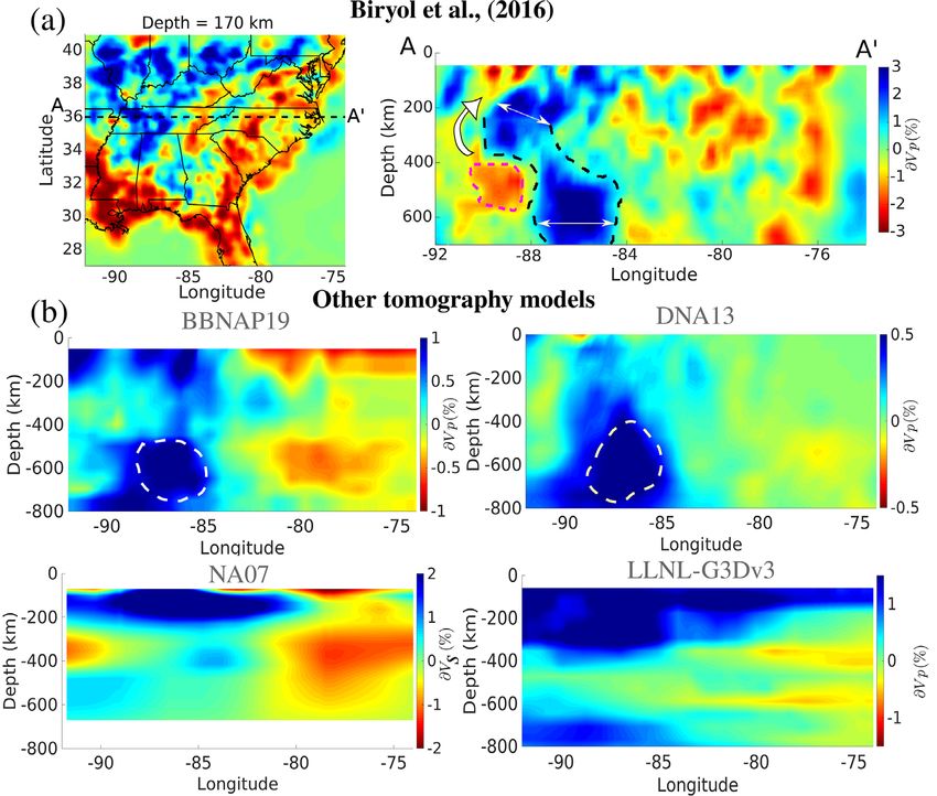
Figure 1. A shaded relief map of the study area including the central occurring between 2011 and 2015 with moment magnitude, Mw >
and southeastern U.S. seismic zones: New Madrid Seismic Zone (NMSZ), 5.5. The discretized model grid has a lateral extent of 30 km in
eastern Tennessee Seismic Zone (ETSZ) South Carolina Seismic Zone the centre and 45 km along the boundary of the domain. The depth
(SCSZ), Giles County Seismic Zone (GCSZ) and Central Virginia Seis- extent of the grid is from 36 to 915 km and consists of 21 layers,
mic Zone (CVSZ). White dashed line represents the well-sampled region
but we are only interested in the features extending down to 660 km
in the tomography results by Biryol et al. (2016) at a depth 130 km.
The earthquakes that occurred over the period December 2011–December
for this study. The tomographic inversion algorithm is described in
2018 and had Mw > 2.5 are plotted as coloured circles. The size and detail in the supplementary information by Biryol et al. (2016). Only
colour of a circle represent the event’s magnitude and depth. The earth- model nodes with high quality (hit points) are used, and therefore,
quake catalog is obtained from the United States Geological Survey at only model results deeper than 60 km depth are interpreted by Biryol
https://earthquake.usgs.gov/earthquakes/search/, where earthquakes with et al. (2016).
Mw > 2.5 in the United States are published. Biryol et al. (2016) evaluate their inversion results with resolution
tests. The well-sampled region in the tomographic inversion shows
to set up numerical models, and found that lithospheric heterogene- high-velocity anomalies with a mean amplitude of 1.9 per cent,
ity plays a crucial role in predicting the intraplate seismicity for the which are interpreted as lithospheric foundering (Fig. 2a). The
Western United States. vertical cross-sections in Fig. 2 show that these anomalies start
Similar considerations of crustal and mantle stress sources are yet at ∼200 km depth with lateral dimensions of ∼2◦ and extend to
to be made for other CEUS seismic zones such as the ETSZ, SCSZ, 660 km where they widen to ∼3◦ (marked in Fig. 2a). According to
GCSZ and CVSZ. In a recent high-resolution P-wave tomography the synthetic anomaly tests, the supposed foundering lithospheric
study, Biryol et al. (2016) found positive velocity anomalies in drip with these amplitudes and dimensions should be reliably re-
the upper mantle beneath the area in-between the ETSZ and the solved.
NMSZ at depths of 200–660 km, and interpreted them as foundering We also assess the performance of the regional tomography model
lithosphere. They further speculated that, since the NMSZ and the by Biryol et al. (2016) using global and contiguous U.S. tomography
ETSZ coincide with the boundaries of lithosphere thinned by the models. Fig. 2 shows the vertical cross-section along latitude 36◦ for
drip, they are weakened by the underlying hot asthenosphere and four different tomography models: BNAP19 (P-wave tomography
thus prone to seismicity. model of the continental U.S. concentrating on the upper mantle
In this study, we investigate the effects of the upper mantle het- structure by Boyce et al. 2019), DNA13 (P-wave and S-wave veloc-
erogeneities found in the P-wave tomography study by Biryol et al. ity model for the contiguous United States by Porritt et al. 2014),
(2016) on the seismicity in the CEUS. Using 3-D numerical mod- NA07 (S-wave velocity model of the upper mantle in North America
els, we compute differential stress, Coulomb stress, gravitational by Bedle & van der Lee 2009), and LLNL-G3Dv3 (Global P-wave
potential energy (GPE), dynamic topography and rate of dynamic tomography model by Simmons et al. 2012). The high-velocity
topography arising from the mantle flow generated from the hetero- anomalies observed by Biryol et al. (2016) can also be seen in the
geneous temperature (or equivalently, density) variations converted BBNAP19 and DNA13 tomography models (dashed white lines in
from the tomography model. Following previous studies that have Fig. 2). However, the colour scales in both the BBNAP19 (∂Vp
demonstrated correlation between differential stress (e.g. Baird et al. = ±1 per cent) and DNA13 (∂Vp = ±0.5 per cent) models clearly
2010; Zhan et al. 2016), deviatoric stresses (e.g. Levandowski et al. show that the high-velocity anomaly is resolved in much higher
2016), or topographic changes (Becker et al. 2015; Ghosh et al. detail (∂Vp = ±3 per cent) in the Biryol et al. (2016) model. A
2019) with the observed intraplate seismicity, we will consider con- correspondence between the Biryol et al. (2016) model and NA07
tributions of the upper mantle heterogeneity to these stress fields, and LLNL-G3Dv3 models is not observed. This is understandable
GPE, dynamic topography, and rate of dynamic topography. Ghosh as NA07 is a shear wave velocity model while Biryol et al. (2016)
et al. (2019) took a similar approach using different lateral viscosity utilize P-wave traveltimes, and LLNL-G3Dv3 is a global tomogra-
models, and studied how their predicted deviatoric stresses arising phy model extending to the core–mantle boundary, which makes it
from long wavelength density variations in the lithosphere and the difficult to resolve regional anomalies.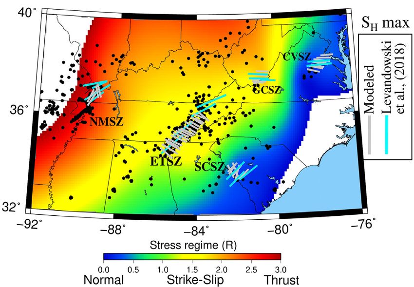
1626        A. Saxena et al.

                                                                                                                                                                     Downloaded from https://academic.oup.com/gji/article/225/3/1624/6166784 by guest on 26 May 2021
Figure 2. (a) P-wave tomography results by Biryol et al. (2016) for a layer at 170 km (left-hand panels) and a cross-section A–A through latitude 36◦
(right-hand panels). Dashed black line on the cross-section marks the approximate boundaries of the high-density anomalies interpreted as a foundering
lithospheric root. Dashed magenta line indicates the low-velocity region interpreted by Biryol et al. (2016) as asthenospheric return flow due to the foundering
lithosphere. The thick white arrow shows the direction of the return flow as speculated by Biryol et al. (2016) and the thin white arrows shows the lateral extent
of the anomaly discussed in the text. (b) Cross-sections along 36◦ N of the published tomography models, BBNAP19, DNA13, NA07 and LLNL-G3Dv3. Data
were retrieved from the IRIS data management centre https://ds.iris.edu/ds/products/emc/ (Trabant et al. 2012). See the main text for more information and
references for each model. The white dashed lines in the BBNAP19 and the DNA13 models show the outline of the high-density anomaly observed in detail
by Biryol et al. (2016).

3 M O D E L L I N G I N S TA N TA N E O U S
M A N T L E F LOW

3.1 Temperature calculations
Inferring temperature from the seismic velocity anomalies has pri-
mary importance for our modelling approach because it will deter-
mine both the driving buoyancy force and the viscous resistance.
We follow Cammarano et al. (2003)’s approach, with a few excep-
tions, to calculate temperatures from the seismic velocity anomalies.
This approach takes into account the effects of anharmonicity (i.e.
elasticity), anelasticity and the phase transition at 410 km depth. In-
version of seismic tomography to a temperature field is commonly
regarded as a non-linear problem due to the shear anelasticity of
seismic waves (Minster & Anderson 1981; Karato 1993; Sobolev
et al. 1996; Goes et al. 2000; Artemieva et al. 2004) and non-linear
sensitivity of elastic moduli and their pressure derivatives to temper-
ature (Duffy & Anderson 1989; Anderson et al. 1992; Cammarano
et al. 2003; Stixrude & Lithgow-Bertelloni 2005). The presence
of melt or water may also introduce non-linearity in temperature
effects on seismic velocities (Karato & Jung 1998) but the effects                  Figure 3. Depth profile of the laterally averaged P-wave velocity sensitivity
of melt and fluids are not considered in this study because of the                  to temperature. See text for the details of calculations.
lack of high heat flow and other substantial evidence for melting
in this region of the mantle (Blackwell et al. 2006). Our inversion                 found to be −0.80 per cent per 100◦ K and −0.62 per cent per 100◦ K
procedure is fully detailed in Appendix A.                                          at two representative depth layers of 200 and 605 km, respectively.
   The laterally averaged scaling of velocity anomalies to the in-                  These values are consistent with those in Cammarano et al. (2003):
verted temperatures (∂Vp/∂T) is shown in Fig. 3. The non-linear                     −0.75 ± 0.15 per cent per 100◦ K and −0.65 per cent per 100◦ K
sensitivity of P-wave velocity anomalies to temperature perturba-                   at the same depths, along the mantle adiabats 1300 and 1600 ◦ C,
tions with depth can be seen from Fig. 3. The average ∂Vp/∂T is                     respectively, used in this study.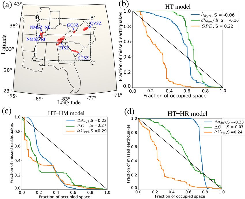
Seismicity in the central and southeastern US             1627

                                                                               pressure. In this rheology model, the effective viscosity (ηeff ) is
                                                                               computed as (Billen & Hirth 2007):

                                                                                     1 − n1i mn i 1−n  i       E i + P Vi
                                                                               ηi = Ai d ε˙i   i    ni
                                                                                                         exp                , i = diff or dis,  (1)
                                                                                     2                            n i RT
                                                                                                    −1
                                                                                         1        1
                                                                               ηeff =         + dis       ,                                     (2)
                                                                                        ηdiff    η
                                                                               where diff and dis denote diffusion and dislocation creep, Ai is the
                                                                               pre-exponential factor, ni is the power law exponent, d is the grain
                                                                               size, mi is the grain size exponent, ε̇ is the second invariant of the
                                                                               strain rate tensor, R is the gas constant, T is temperature obtained
                                                                               from the inversion of the Vp anomalies, P is pressure and Ei and Vi
                                                                               are the activation energy and volume, respectively. All the parameter
                                                                               values used in this study are given in Table 1.
                                                                                  It should be noted that our modelled viscosities are dependent on

                                                                                                                                                        Downloaded from https://academic.oup.com/gji/article/225/3/1624/6166784 by guest on 26 May 2021
                                                                               the temperature distribution inverted from the tomography model
                                                                               (described in Appendix A). The distinction between the lithospheric
Figure 4. Model domain and cross-sections of the modelled viscosity using      mantle and the sublithospheric mantle is included in our model by
the temperatures based on the regional tomography by Biryol et al. (2016).     the temperature change with depth, and therefore, by the computed
Grey isosurface represents P-wave anomalies >2 per cent in the region          viscosities. We do not consider a crustal compositional layer because
interpreted as lithospheric foundering. The state boundaries are drawn in      the tomography model considers only the upper mantle starting from
solid black and red dots are epicentres for the earthquake catalogue used in   a depth of 36 km; there are no lateral variations in the viscosity in
Fig. 1. The boundary conditions are annotated on the bottom left.              the crust. This assumption for the crust is appropriate here, since
                                                                               we are interested in the effects of the lateral viscosity variations
                                                                               at deeper depths using differences in model outputs (HT−HM and
3.2 Model setup                                                                HT−HR in Fig. 5).
                                                                                  The bottom boundary at 660 km has the free-slip condition (e.g.
We compute velocity and stress fields that are in equilibrium with
                                                                               Arcay et al. 2007; Billen & Hirth 2007; Quinquis et al. 2011). For
heterogeneous buoyancy forces arising from the heterogeneous
                                                                               side boundaries, we tested our model with both free-slip and no-slip
distribution of temperature-dependent density. For this calcula-
                                                                               conditions and verified that the velocity fields at the seismic zones
tion, we use an open-source finite element code, ASPECT version
                                                                               have the same pattern but up to 5 per cent magnitude difference in
2.0.0 (Kronbichler et al. 2012; Heister et al. 2017; Rose et al. 2017;
                                                                               our region of interest. In this study, we only show the results for
Bangerth et al. 2018). ASPECT can solve the equations for the con-
                                                                               the no-slip conditions. We let the top boundary be a free surface,
servation of mass, momentum and energy using an adaptive finite
                                                                               which was developed by Rose et al. (2017) in ASPECT, that can
element method for a variety of rock rheologies.
                                                                               generate topography in response to the instantaneous flow in the
   Our model domain is laterally bounded by longitudes, 71◦ W and
                                                                               mantle.
95.5◦ W and by latitudes, 23◦ N and 43◦ N. The depth range is from
0 to 660 km (Fig. 4). The domain is discretized into 0.512 million
hexahedral elements with a 0.15◦ resolution in longitude, 0.125◦
                                                                               3.3 Geodynamic quantities
in latitude and 35 km in depth. This spatial resolution is similar to
that of the tomography and thus, sufficient for resolving the mantle           We compute three measures from our numerical model to be tested
velocity structure shown by the tomography model.                              for their relevance to seismicity: GPE, dynamic topography and rate
   We assessed mesh resolution effects by running a model with a               of change of dynamic topography. We also compute three stress
two times finer mesh having 2.048 million elements and found that              indicators: Differential stress, Coulomb stress at observed fault ge-
differences in the results were small, amounting to a relative error           ometries and optimal Coulomb stress in models isolating the effects
of 2 per cent in the velocity field. All the model results presented           of upper mantle heterogeneity and the foundering lithosphere. We
in this study are thus based on the coarse mesh for computational              collectively refer to these six quantities as geodynamic quantities in
efficiency. We also tested a model with an additional lateral area             this study.
of 5◦ by 5◦ surrounding our domain to asses boundary effects.                     Molchan curves (Molchan 1990, 1991) and their associated skill
The overall resultant velocity and stress field are similar to those           (S) (Becker et al. 2015) are computed to quantify the earthquake
for the smaller model domain, but the magnitude of the calculated              prediction power of the six geodynamic quantities listed above.
stress and velocity field at our depth of interest (15 km) near the            The predicting quantity (‘predictor’) is first expressed as a fraction
boundaries is smaller by 10–15 per cent because the viscous effect             of ‘occupied’ space where the predictor is less than or equal to a
of the same heterogeneity is now spread over a larger area. However,           value in the space. This mapping implies that the maximum and the
since the seismic zones are sufficiently far from the model domain             minimum value of the predictor has occupied space equal to 1 and 0,
boundaries, we show only the results for the smaller domain.                   respectively. Next, we find the fraction of earthquakes that occurred
   The upper mantle is typically assumed to deform by a dislocation            outside the space occupied by the value of the predictor, referred to
creep at low temperatures relative to the melting temperatures of              as the fraction of missed earthquakes. We define a Molchan curve
mantle rocks and by a diffusion creep at higher temperatures with              as a plot of fractions of missed earthquakes against fractions of
respect to the melting temperatures (e.g. Gordon 1967). Our model              occupied space. When the occupied space fraction of a geodynamic
uses a composite rheology with both dislocation and diffusion creep            quantity is 0, all the earthquakes will be missed so the fraction of
having different contributions depending on the temperature and                missed earthquakes is 1. When the occupied space fraction is 1,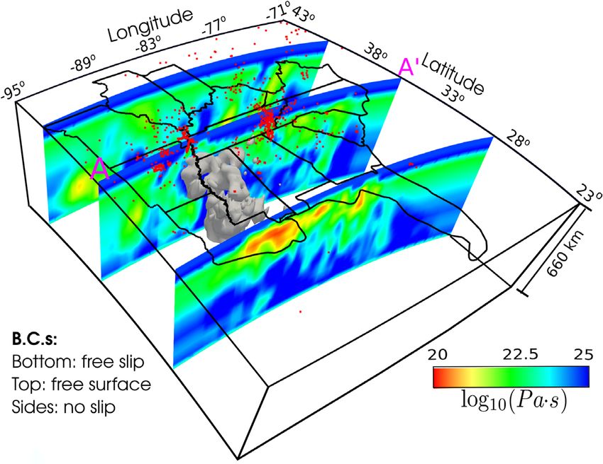
1628        A. Saxena et al.

                            Table 1. Values of parameters for dislocation and diffusion creep.
                            Parameter                         Symbol           Unit         Diffusion creep       Dislocation creep
                            Pre-exponential factora              A             s−1            1.5 × 10⁻¹⁶            0.3 × 10⁻²²
                            Power law exponenta                  n                                 1                     3.5
                            Grain size exponenta                 m                                 2                       0
                            Activation energya                   E         kJ mol−1               300                    530
                            Activation volumea                   V                                 6                      20
                                                                          cm3 mol−1
                            Grain sizeb                          d          mm                     5                      5
                            Note: a Karato & Wu (1993). b Approximate value for olivine (Karato 1984).

                                                                                                                                                                Downloaded from https://academic.oup.com/gji/article/225/3/1624/6166784 by guest on 26 May 2021
Figure 5. Cross-section along 36◦ N across three models: HeTerogeneous (HT), homogeneous mantle (HM) and homogeneous root (HR) models. Stress
changes in HT are computed relative to HM (HT−HM) or to HT (HT−HR). HT−HM represents the effects of the whole upper mantle heterogeneity and
HT−HR those of the lithospheric drip only.

the space will include all the earthquakes, making the fraction of                    3.3.2 Dynamic topography and its rate
missed earthquakes equal to 0. This implies that these curves are
                                                                                      The dynamic topography for our model is computed in AS-
fixed with the boundary conditions of {0,1} and {1,0}. The skill
                                                                                      PECT (Austermann et al. 2015). This quantity represents the ra-
for each predictor is computed as the area of the curve above the
                                                                                      dial stress at the surface due to the mantle flow generated from
Molchan curve minus 0.5, such that a pure random predictor has S
                                                                                      the buoyancy effects based on the heterogeneous temperature dis-
= 0, a pure correlation has S = 0.5, and a pure anti-correlation has S
                                                                                      tribution in the model (Fig. S1). We compute the rate of dynamic
= −0.5. In this study, the Molchan curves are computed collectively
                                                                                      topography by computing the change in dynamic topography be-
for all the seismic zones of the CEUS (Fig. 6a).
                                                                                      tween our instantaneous model and our model run forward in time
                                                                                      for 10 000 yr (Becker et al. 2015, Fig. S1).

                                                                                      3.3.3 Differential and Coulomb stress changes
3.3.1 Gravitational potential energy                                                  We define static Coulomb stress changes (C) for a model with re-
We calculate GPE per unit area in our model domain (Fig. S1)                          spect to another model as the difference in Coulomb failure function
following the thin-sheet approximation described in Ghosh et al.                      (CFF, King et al. 1994):
(2009) as:
                                                                                      C = τ − μ σn ,                                                 (4)
           L
                                                                                      where τ and σ n are the difference between the models in shear
GPE =           zρ(z)gdz,                                                (3)
         −h
                                                                                      (positive in the direction of slip) and normal (positive when com-
                                                                                      pressive) stress, respectively, for a particular fault orientation, and
where ρ(z) is the density at a depth z, g is the acceleration due                     μ is the effective coefficient of friction after accounting for pore
to gravity taken as 9.8 m s–2 , h is the surface topography and L                     pressure. Since we do not have sufficient constraints on the effective
is the assumed compensation depth used as 200 km. We choose                           friction coefficients (μ) for the faults in the study area, we use a
this depth to represent the approximate thickness of the lithosphere                  value of 0.6 as done by Hurd & Zoback (2012) and Huang et al.
for the continents (McKenzie et al. 2005). Due to unavailability                      (2017) for a similar study region. At lower μ, as suggested in the
of the crustal structure in the tomography model by Biryol et al.                     western United States (Townend & Zoback 2004), the faults would
(2016), we use the CRUST1.0 (Laske et al. 2013) model for crustal                     fail easier. Therefore, our choice of μ conservatively computes the
thickness and density distribution, and a lithospheric mantle with                    CFF for our numerical models. CFF values are computed for the
density distribution computed from the seismic tomography (see                        selected fault geometries based on the focal mechanisms and earth-
Appendix A for details).                                                              quake relocations (Table 2) at 15 km depth in all the seismic zones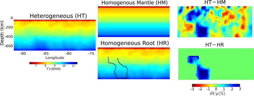
Seismicity in the central and southeastern US               1629

                                                                                                                                                                 Downloaded from https://academic.oup.com/gji/article/225/3/1624/6166784 by guest on 26 May 2021
Figure 6. (a) Locations of the CEUS seismic zones plotted on the top surface of the model domain. Red dots are the nodes of the mesh that belong to the
CEUS seismic zones for which the Molchan curves of Coulomb stress and the optimal Coulomb stress are computed. The box BB’CC’ indicates the region for
which all the other Molchan curves are calculated. (b) Molchan curves for dynamic topography (hdyn ), the rate of dynamic topography change (dhdyn /dt) and
gravitational potential energy (GPE) for the HT model. (c) Molchan curves for change in differential stress (σ diff ), Coulomb stress change for the observed
fault orientations at each seismic zone (Table 2) (C) and Coulomb stress change for the optimal fault geometry where the shear stress is maximum (Copt ).
All are computed for HT−HM. (d) Same as (c) but for HT−HR.

Table 2. Dominant fault geometries in the CEUS seismic zones.∗
Seismic zone         Strike, dip                       Sense of motion                     Reference
NMSZ NE              N10◦ E, 90◦                       right-lateral                      Chiu et al. (1992); Shumway (2008)
NMSZ RF              N167◦ E, 30◦ SW                   thrust                             Csontos & Van Arsdale (2008)
ETSZ                 1- N10◦ E, 90◦ ; 2- E-W, 90◦      right-lateral; left-lateral        Chapman et al. (1997); Cooley (2015); Powell & Thomas (2016)
GCSZ                 E-W, 90◦                          left-lateral                       Munsey & Bollinger (1985)
CVSZ                 N30◦ E, 50◦ SE                    thrust                             Wu et al. (2015)
SCSZ                 N180◦ E, 40◦ W                    thrust                             Chapman et al. (2016)
Note: ∗ NMSZ NE, North eastern arm of New Madrid Seismic Zone; NMSZ RF, Reelfoot fault of the New Madrid Seismic Zone; ETSZ, Eastern Tennessee
Seismic Zone; GCSZ, Giles County Seismic Zone; CVSZ, Central Virginia Seismic Zone; SCSZ, South Carolina Seismic Zone.

(Figs S3 and S4). The details of the Coulomb stress computation                      setups. Coulomb stress changes, CHT − HM and CHT − HR , indi-
are in Appendix B. Differential stress, σ diff ≡ σ 1 − σ 3 , is compared             cate whether and how much the stress field in the model HT would
between different models with a similarly defined quantity, σ diff .                promote the slip tendency of a fault relative to stress fields in HM
   To facilitate comparison of models with and without the local                     and HR. For instance, a positive CHT − HM for a fault geometry
upper-mantle heterogeneity, delineated by the velocity anomaly iso-                  and a sense of motion means that the mantle heterogeneities con-
surface in Fig. 4, we denote our reference model with tomography-                    sidered in HT promote the failure of the fault relative to the laterally
based temperatures plus the reference geotherm as HT (HeTeroge-                      homogeneous mantle (HM).
neous), a model with the reference geotherm in the upper mantle
as HM (HoMogeneous), and a model identical with HT except
that the temperature within the foundering lithosphere is replaced                   3.3.4 Optimal Coulomb stress
with the reference geotherm values as HR (Heterogeneous but                          We define the optimal fault orientation as the one maximizing the
having no Root). HT−HM represents the contributions from the                         Coulomb stress changes of HT relative to HM (CHT − HM ), and
mantle flow generated only due to the upper mantle heterogene-                       for HT relative to HR (CHT − HR ). We calculate the optimal fault
ity (>60 km), while HT−HR shows only the contribution of the                         orientation using a grid search over strikes from N90◦ E to S90◦ E and
high-velocity structure interpreted as the foundering drip. Fig. 5                   dips from 10◦ to 90◦ at an interval of 10◦ for the possible senses of
shows a cross-section of the tomography illustrative of these model                  motion: right- and left-lateral strike-slip, normal and thrust faulting.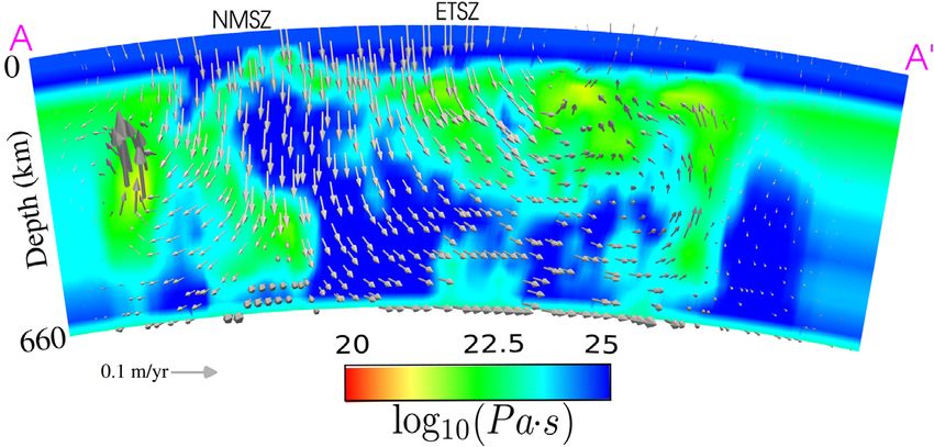
1630       A. Saxena et al.

The optimal fault orientation could also be calculated analytically
using two successive stress rotations (one to align a plane at a strike
angle and then a rotation to a fault dip), and then solving for the
strike and dip angles that maximize the C. Since we are also
interested in the C distribution over the range of strikes and dips,
we use the grid search method.

4 M O D E L R E S U LT S
The Molchan curves for the geodynamic quantities, except the
Coulomb stress and the optimal Coulomb stress, are computed for
all the model points in the seismic zones of the CEUS: ETSZ, SCSZ,
CVSZ, GCSZ and NMSZ (shown in Fig. 6a) which are contained
in the well-resolved region in the Biryol et al. (2016) tomography.
Since each seismic zone has a corresponding fault geometry, only

                                                                                                                                                          Downloaded from https://academic.oup.com/gji/article/225/3/1624/6166784 by guest on 26 May 2021
the points within that seismic zone are accounted for when calcu-
                                                                              Figure 7. Maximum horizontal stress directions (SH max) from the HT
lating the Molchan curves of the Coulomb stress and the optimal
                                                                              model (grey lines) at 15 km depth and from the focal mechanism inversion
Coulomb stress (Fig. 6a).                                                     study by Levandowski et al. (2018) (magenta lines). The background colour
   The geodynamic quantities, GPE, hdyn and dhdyn /dt, are computed           map represents the stress regime parameter (R) for the model HT at 15 km
at the top surface for our reference model, which is based on the             depth. The white areas are the regions where R is not computed.
tomography converted temperatures and viscosities (HT, Fig. 5) in
Fig. S1. Both the dynamic topography and its rate show negative
                                                                              = −0.06, the dynamic topography itself is not a good predictor,
skills for prediction of earthquakes (Fig. 6b). The skill of dynamic
                                                                              either. This contrast in the predicting powers of vertical stress at
topography is −0.06 and that of the rate of dynamic topography is
                                                                              the top surface (hdyn and dhdyn /dt) and the GPE indicates that the
even more negative, −0.16. The GPE shows a high positive skill of
                                                                              CEUS seismic zones are better correlated with lithospheric mantle
S = 0.22.
                                                                              or crustal density heterogeneities than with the stresses arising due
   Changes in the stress indicators, differential and Coulomb stress,
                                                                              to sublithospheric mantle flow (i.e. deeper bouyancies). Although
for the HT−HM case are computed at a depth of 15 km (Figs S3
                                                                              further study is needed, our finding also suggests that the rate of
and S5), at which seismicity in the study area is most frequent (e.g.
                                                                              dynamic topography might be a useful indicator of seismicity in a
Mazzotti & Townend 2010). The Coulomb stress changes, C,
                                                                              rather special situation such as in the tectonically active Western
in Figs S4 and S5 are calculated for each seismic zone using the
                                                                              United States.
corresponding fault geometries mentioned in Table 2. These stress
                                                                                 The overall skill associated with the stress indicators of the
changes account for the effects from heterogeneities in the entire
                                                                              HT−HM model (Fig. 6c) is stronger than the HT−HR model
upper-mantle. Molchan curves for σ diff , C and Copt are shown
                                                                              (Fig. 6d). This is consistent with the high skill measure of the GPE
in Fig. 6(c); and the skills of all three indicators are strongly positive:
                                                                              in the HT model (Fig. 6b), since the total mantle density anomalies,
0.22, 0.27 and 0.29, respectively.
                                                                              as accounted in the HT−HM model, give rise to the GPE. Differ-
   Stress indicators computed for the HT−HR case are plotted in
                                                                              ential stress change for the HT−HM model, σdiff     HT−HM
                                                                                                                                          , shows a
Figs S4 and S6 and their corresponding Molchan curves in Fig. 6(d).
                                                                              positive correlation with the observed seismicity (Fig. 6c). On the
These stress changes represent the isolated effects of the lithospheric
                                                                              other hand, the lithospheric drip alone has a negative correlation
drip. σ diff negatively correlates (S = −0.23) with the observed
                                                                              with the earthquake locations in this region (Fig. 6d). Although the
earthquake distribution. C for the observed fault geometries shows
                                                                              positive values of differential stress changes suggest an increased
minimal correlation (S = −0.07) with the seismicity, while Copt
                                                                              potential for seismicity, even the greatest value of σdiff
                                                                                                                                      HT−HM
                                                                                                                                               ∼ 30
shows a highly positive skill, 0.24.
                                                                              MPa in the ETSZ (Fig. S2) is an order of magnitude less than the
                                                                              value required for the generation of faults at crustal depths of 10–
                                                                              20 km (using appropriate values for crust in Byerlee’s Law). This
5 DISCUSSION
                                                                              deficiency in magnitude requires other contributions for explaining
The Molchan analyses of the geodynamic quantities for our models              the seismicity in the CEUS like weak existing faults created dur-
suggest that GPE is the best indicator of the seismicity, implying            ing the past several Wilson cycles (Thomas et al. 2006) or long
a good correlation between the seismicity and the areas of high               wavelength boundary stresses as suggested by Ghosh et al. (2019).
GPE (highest skill, S = 0.22, in Fig. 6b). The GPE values repre-              From our Coulomb stress change calculations for the observed fault
sent the integrated vertical stress arising from the laterally varying        geometries of the seismic zones (Table 2), we find that these faults
lithospheric densities. The high GPE areas have more earthquakes              are more loaded towards failure in the heterogeneous upper mantle
because these are also the regions with thinned crust, and therefore,         relative to a homogeneous upper mantle (Fig. 6c, S3). As expected
thicker high-density lithospheric mantle, based on the tomography             from the definition of the optimal Coulomb stress (Copt ), the skill
model used in this study (fig. 10 in Biryol et al. 2016). The high            for both the cases HT−HM and HT−HR at each seismic zone is
predicting power of GPE suggests that the lateral density and thick-          maximum among all the stress indicators (Figs 6c and d).
ness variations of the lithosphere are important factors to consider             We compare the directions of maximum horizontal stress
in understanding the earthquake generation in the CEUS. Although              (SH max) computed from the model HT at the depth of 15 km,
the rate of dynamic topography showed a good correlation with                 the depth at which most earthquakes in this region occur (Mazzotti
seismicity in the western United States (Becker et al. 2015), its             & Townend 2010), with the SH max from the study by Levandowski
skill in the model HT is negative, S = −0.16 (Fig. 6b). With S                et al. (2018) (Fig. 7). These authors utilized focal mechanisms for
Seismicity in the central and southeastern US 1631
downward flow due to the lithospheric drip is not consistent with
the asthenospheric upwelling that Biryol et al. (2016) proposed
would occur as a counter-flow to the drip. However, asthenopsheric
upwelling cannot be reliably rejected because the velocity field in
our model depends on various parameters including the viscosity of
the asthenosphere and the boundary conditions. Lower viscosity of
the asthenosphere, for instance, would reduce the lateral extent of the
downward drag by the lithospheric drip such that the region beneath
the NMSZ might not be affected as strongly as in the current model.
We ran models with only diffusion creep and only dislocation creep
and found similar flow directions but a different flow law might alter
Figure 8. Velocity (arrows) and viscosity fields from the model HT on the
the flow pattern around the high-density foundering lithosphere. A
slice AA (marked on Fig. 4). Large velocities observed west of the NMSZ model with depth dependent viscosity with a high viscosity layer
and out of the plane correspond to the upward return flow in reaction to the in the transition zone would inhibit a downward flow from the
downward pull of the lithospheric drip. high-density lithospheric drip, making the velocity vectors turn at
shallower depths.
Downloaded from https://academic.oup.com/gji/article/225/3/1624/6166784 by guest on 26 May 2021
the contiguous United States to obtain their stresses. The SH max val- Forte et al. (2007) presented numerical models involving vis-
ues from our model roughly match those obtained by Levandowski cosities based on the joint inversion of seismic and geodynamic
et al. (2018) in all the seismic zones but the ETSZ (Fig. 7). The angu- data and observed a downward vertical flow beneath the NMSZ,
lar deviation of our modelled SH max values with the inverted SH max that interacts with the overlying lithosphere to generate seismicity.
results averaged over each seismic zone considered in Fig. 7 is ap- Comparing our flow field with the results from Forte et al. (2007),
proximately 20◦ , 68◦ , 4◦ , 12◦ and 15◦ for the NMSZ, ETSZ, GCSZ, we can see a similar vertical flow at depths of 300–500 km, but
CVSZ and SCSZ, respectively. SH max based on HT is NNW–SSE the velocity patterns at shallower depths differ significantly. A pos-
in the ETSZ, differing from the NE–SW direction determined us- sible reason for the mismatch is the difference in the tomography
ing focal mechanism solutions by Levandowski et al. (2018) and studies utilized for the numerical models. Our study incorporates
by Mazzotti & Townend (2010). This misfit in the SH max of the a regional tomography model (Biryol et al. 2016), while the Forte
ETSZ has also been observed by Ghosh et al. (2019) (Fig. 7 of the et al. (2007) model is a global model focusing on much larger
paper) in their numerical models with lateral viscosity contrasts in wavelength anomalies.
the crust and the upper mantle. A possible reasoning for this misfit This study focuses on the contribution from local stress pertur-
is stress concentration along the boundary of the strength contrast bations due to the upper mantle heterogeneities on the seismicity
in the basement crustal rocks (Powell et al. 1994), which is difficult of the CEUS. Other likely mechanisms to explain the earthquakes
to resolve in a global tomography study used by Ghosh et al. (2019) in this region include the presence of spatially limited weak zones
or a regional mantle tomography study used here. activated under plate boundary stresses, and stress concentrations
The distribution of stress regime parameter, R, (Delvaux et al. due to large-scale viscosity variations, such as cratons and plate
1997; Simpson 1997), computed based on the model HT at 15 km boundaries. The idea of finite weaknesses under far-field stress has
depth, shows that the dominant faulting styles are thrust for the been studied previously by Kenner & Segall (2000) and Zhan et al.
NMSZ NE, and oblique-thrust for the GCSZ (Fig. 7). These (2016) for the NMSZ. Kenner & Segall (2000) proposed a model
stress regimes are consistent with the proposed faulting styles with a weak lower crustal zone within an elastic lithosphere that
in Levandowski et al. (2018) for these zones, but differ from the acts as a local source of stress concentration from the far-field
selected studies in Table 2 which suggest strike-slip for the GCSZ stresses. Similarly, based on a regional tomography model by Pol-
and the NMSZ NE. The HT model predicts normal faulting at litz & Mooney (2014), Zhan et al. (2016) found that weak upper
the SCSZ and the CVSZ. These zones are associated with thrust mantle inferred from low seismic velocities can focus stress in
faulting in Levandowski et al. (2018), and the studies mentioned the NMSZ crust. Ghosh et al. (2019) found that large-scale litho-
in Table 2. This discrepancy between the modelled and predicted spheric structure variations (and, therefore, viscosities) could alter
faulting style at the CVSZ and the SCSZ occurs because our model the strain-rates, and affect the seismicity of the CEUS. The regional
does not account for compressive tectonic stresses due to ridge stress direction is northeast–southwest compressive stress for the
push and long-wavelength crustal and mantle viscosity contrasts CEUS (Zoback & Zoback 1989). It might be possible to superim-
(i.e. between cratons and weak plate boundaries), which are highest pose the contributions from the plate boundary, large-scale stress
at these zones due to the proximity to the plate boundary. Within sources, and local stress sources for a first-order understanding us-
the ETSZ, a strike-slip mechanism has been suggested by other ing a viscoplastic model that accounts for pre-existing weaknesses.
studies (Chapman et al. 1997; Mazzotti & Townend 2010; Powell However, our model is based on the upper-mantle tomography study
& Thomas 2016) which agrees with our model result, but differs and does not account for the spatially limited crustal weak zones
with Cooley (2015) and Levandowski et al. (2018) who find nor- (fault zones), or the stress concentration from the large-scale mantle
mal faulting in the ETSZ. This discrepancy may be because Cooley flow. This complexity is outside the scope of this study and is not
(2015) and Levandowski et al. (2018) consider new focal mech- addressed further.
anism data in their stress inversions indicating a propensity for Time dependent modelling will be needed to address the mech-
normal faulting in the ETSZ. anism for the origin of a foundering drip in the CEUS. It has been
A broad downward flow is found below both the NMSZ and ETSZ proposed by Biryol et al. (2016) that the lithospheric foundering
in the velocity field (Fig. 8) in the cross-section AA of the model could have started due to Rayleigh-Taylor instability associated
HT (marked in Fig. 4). The descending flow induces upwellings with the presence of an eulogized root as proposed by Le Pourhiet
along the edges of the model domain. The upwellings are observed et al. (2006) in the western United States. Such an investigation
at the surface as features F1 and F2 marked in Fig. S2. The broadly in this region would call for more sophisticated techniques such as1632 A. Saxena et al.
backward advection modelling (e.g. Conrad & Gurnis 2003), quasi- AC K N OW L E D G E M E N T S
reversibility (Glišović & Forte 2016) or adjoint methods (e.g. Bunge
We thank Dr Thorsten W. Becker, Dr Attreyee Ghosh, and two
et al. 2003; Liu et al. 2008) for the calculation of initial conditions
anonymous reviewers for their detailed review, which has greatly
on temperature, viscosity and density, which has not been done in
improved the quality and analysis of our study. We are grateful to Dr
this study.
Berk Biryol for sharing their tomography results used for modelling
It is also possible that the dense high-velocity mantle feature
in this study. We also thank the Computational Infrastructure for
imaged by Biryol et al. (2016) is part of the subducted Farallon
Geodynamics (geodynamics.org) which is funded by the National
slab below this region (Schmid et al. 2002; Mooney & Kaban 2010;
Science Foundation under award EAR-0949446 and EAR-1550901
Sigloch et al. 2008; Schmandt & Humphreys 2010; Sigloch 2011).
for supporting the development of ASPECT. The parameter file for
Schmid et al. (2002) used kinematic thermal modelling to track the
the final reference model, HT and the jupyter notebook created for
subduction history of the Farallon slab and found that the Farallon
the inversion of seismic tomography is available at https://github.c
lithosphere continues to the central United States and is still a
om/alarshi/ceus seismicity.
negative thermal anomaly observable in the seismic tomography
studies. Mooney & Kaban (2010) computed the gravity signal from
the upper mantle for North America and observed a large gravity
high in the southeastern United States, which they attributed to the
Downloaded from https://academic.oup.com/gji/article/225/3/1624/6166784 by guest on 26 May 2021
east-dipping Farallon slab. Schmandt & Humphreys (2010) present
REFERENCES
Vp and Vs tomographic images for the western United States and Anderson, O.L., Isaak, D. & Oda, H., 1992. High-temperature elastic con-
interpret their positive velocity anomalies in the Rockies as the stant data on minerals relevant to geophysics, Rev. Geophys., 30(1), 57–90.
eastward dipping segmented Farallon slab. Sigloch et al. (2008); Arcay, D., Tric, E. & Doin, M.-P., 2007. Slab surface temperature in subduc-
Sigloch (2011) present P-wave tomography for North America to tion zones: influence of the interplate decoupling depth and upper plate
a depth of 1800 km, and interpret a high-velocity anomaly in the thinning processes, Earth planet. Sci. Lett., 255(3–4), 324–338.
CEUS at the mantle transition depths as a stagnant fragment of the Artemieva, I.M., Billien, M., Lévêque, J.-J. & Mooney, W.D., 2004. Shear
Farallon slab. We do not comment on the origin of this high-velocity wave velocity, seismic attenuation, and thermal structure of the continental
feature but follow the naming convention by Biryol et al. (2016) as upper mantle, Geophys. J. Int., 157(2), 607–628.
Austermann, J., Pollard, D., Mitrovica, J.X., Moucha, R., Forte, A.M., De-
a drip in this study. Additional observations such as low dynamic
Conto, R.M. & Raymo, M.E., 2015. The impact of dynamic topography
topography at the surface would be required to confirm if the high
change on antarctic ice sheet stability during the mid-Pliocene warm
velocity is indeed attached to the lithosphere or is a remnant Farallon period, Geology, 43(10), 927–930.
slab. Baird, A., McKinnon, S. & Godin, L., 2010. Relationship between structures,
stress and seismicity in the Charlevoix seismic zone revealed by 3-D ge-
omechanical models: implications for the seismotectonics of continental
interiors, J. geophys. Res., 115(B11), doi:10.1029/2010JB007521.
6 C O N C LU S I O N S Bangerth, W., Dannberg, J., Gassmoeller, R., Heister, T. et al. , 2018. AS-
In this study, we advance the understanding on the role of upper PECT v2.0.0 [software], doi:10.5281/zenodo.1244587.
mantle stress perturbations in the generation of intraplate seismic- Becker, T.W., Lowry, A.R., Faccenna, C., Schmandt, B., Borsa, A. & Yu, C.,
2015. Western us intermountain seismicity caused by changes in upper
ity by utilizing the highest upper mantle resolution tomography
mantle flow, Nature, 524(7566), 458–461.
study (Biryol et al. 2016) to date for setting up numerical models
Bedle, H. & van der Lee, S., 2009. S velocity variations beneath North
with laterally heterogeneous viscosity and density. We also explore America, J. geophys. Res., 114(B7), doi:10.1029/2008JB005949.
the isolated effects of upper-mantle heterogeneity and a positive Billen, M.I. & Hirth, G., 2007. Rheologic controls on slab dynamics,
P-wave velocity anomaly, interpreted by Biryol et al. (2016) as Geochem. Geophys. Geosyst., 8(8), doi:10.1029/2007GC001597.
a lithospheric drip in our numerical models. We follow the novel Biryol, C.B., Wagner, L.S., Fischer, K.M. & Hawman, R.B., 2016. Rela-
Molchan analysis approach to quantify various earthquake metrics tionship between observed upper mantle structures and recent tectonic
with their corresponding skills, S, following the work by Becker activity across the Southeastern United States, J. geophys. Res., 121(5),
et al. (2015) in the Western United States. We compute earthquake 3393–3414.
predictors for our numerical models, such as the rate of creation of Blackwell, D.D., Negraru, P.T. & Richards, M.C., 2006. Assessment of
the enhanced geothermal system resource base of the united states, Nat.
dynamic topography and GPE, which have not been investigated in
Resour. Res., 15(4), 283–308.
the previous studies.
Boyce, A., Bastow, I.D., Golos, E.M., Rondenay, S., Burdick, S. & Van der
Our analysis of various earthquake predictors to understand the Hilst, R.D., 2019. Variable modification of continental lithosphere during
seismicity in the CEUS has revealed that the lateral upper-mantle the Proterozoic Grenville Orogeny: evidence from teleseismic P-wave
heterogeneity below this region plays a significant role in increasing tomography, Earth planet. Sci. Lett., 525, 115763.
the differential stress (S = 0.22) and Coulomb stress (S = 0.27) Bunge, H.-P., Hagelberg, C. & Travis, B., 2003. Mantle circulation models
at observed fault geometries. Moreover, we also find that upper with variational data assimilation: inferring past mantle flow and structure
mantle structural heterogeneity and density anomalies measured from plate motion histories and seismic tomography, Geophys. J. Int.,
using GPE (S = 0.22) are important for understanding deformation 152(2), 280–301.
in this region. The stress indicators for the model with only the Cammarano, F., Goes, S., Vacher, P. & Giardini, D., 2003. Inferring upper-
mantle temperatures from seismic velocities, Phys. Earth planet. Inter.,
lithospheric drip do not show correspondence with the observed
138(3–4), 197–222.
seismicity pattern. Therefore, our results indicate that the upper
Chapman, M., Beale, J.N., Hardy, A.C. & Wu, Q., 2016. Modern seismic-
mantle flow generated from all the upper mantle heterogeneity is ity and the fault responsible for the 1886 Charleston, South Carolina,
essential to provide a possible mechanism for reactivation of the earthquake, Bull. seism. Soc. Am., 106(2), 364–372.
faults in the intraplate seismicity of the CEUS. This, in turn, helps Chapman, M., Powell, C., Vlahovic, G. & Sibol, M., 1997. A statistical
to better associate seismic hazard with the seismic zones in the analysis of earthquake focal mechanisms and epicenter locations in the
CEUS. eastern Tennessee seismic zone, Bull. seism. Soc. Am., 87(6), 1522–1536.Seismicity in the central and southeastern US 1633
Chen, C., Zhao, D. & Wu, S., 2014. Crust and upper mantle structure of Karato, S. & Jung, H., 1998. Water partial melting and the origin of the
the New Madrid seismic zone: insight into intraplate earthquakes, Phys. seismic low velocity and high attenuation zone in the upper mantle, Earth
Earth planet. Inter., 230, 1–14. planet. Sci. Lett., 157(3–4), 193–207.
Chiu, J., Johnston, A. & Yang, Y., 1992. Imaging the active faults of the Karato, S. & Wu, P., 1993. Rheology of the upper mantle: a synthesis,
central New Madrid seismic zone using panda array data, Seismol. Res. Science, 260(5109), 771–778.
Lett., 63(3), 375–393. Katsura, T., Yoneda, A., Yamazaki, D., Yoshino, T. & Ito, E., 2010. Adiabatic
Conrad, C.P. & Gurnis, M., 2003. Seismic tomography, surface uplift, and temperature profile in the mantle, Phys. Earth planet. Inter., 183(1–2),
the breakup of Gondwanaland: integrating mantle convection backwards 212–218.
in time, Geochem. Geophys. Geosyst., 4(3), doi:10.1029/2001GC000299. Keller, G., Lidiak, E., Hinze, W. & Braile, L., 1983. The role of rifting in
Cooley, M., 2015. A new set of focal mechanisms and a geodynamic model the tectonic development of the midcontinent, USA, in Developments in
for the eastern Tennessee seismic zone, MS thesis, The University of Geotectonics, Vol. 19, pp. 391–412, Elsevier.
Memphis, Memphis, Tennessee, pp. 1–46. Kenner, S.J. & Segall, P., 2000. A mechanical model for intraplate earth-
Cottaar, S., Heister, T., Rose, I. & Unterborn, C., 2014. Burnman: a lower quakes: application to the New Madrid seismic zone, Science, 289(5488),
mantle mineral physics toolkit, Geochem. Geophys. Geosyst., 15(4), 2329–2332.
1164–1179. Kennett, B. & Engdahl, E., 1991. Traveltimes for global earthquake location
Csontos, R. & Van Arsdale, R., 2008. New Madrid seismic zone fault ge- and phase identification, Geophys. J. Int., 105(2), 429–465.
ometry, Geosphere, 4(5), 802–813. King, G.C., Stein, R.S. & Lin, J., 1994. Static stress changes and the trig-
Downloaded from https://academic.oup.com/gji/article/225/3/1624/6166784 by guest on 26 May 2021
Delvaux, D., Moeys, R., Stapel, G., Petit, C., Levi, K., Miroshnichenko, gering of earthquakes, Bull. seism. Soc. Am., 84(3), 935–953.
A., Ruzhich, V. & Sankov, V., 1997. Paleostress reconstructions and geo- Kronbichler, M., Heister, T. & Bangerth, W., 2012. High accuracy mantle
dynamics of the Baikal region, central Asia, part 2. Cenozoic rifting, convection simulation through modern numerical methods, Geophys. J.
Tectonophysics, 282(1–4), 1–38. Int., 191, 12–29.
Duffy, T.S. & Anderson, D.L., 1989. Seismic velocities in mantle minerals Laske, G., Masters, G., Ma, Z. & Pasyanos, M., 2013. Update on crust1.
and the mineralogy of the upper mantle, J. geophys. Res., 94(B2), 1895– 0–a 1-degree global model of earth’s crust, in Proceedings of the EGU
1912. General Assembly, 7–12 April 2013, Vienna, Austria, Geophys. Res.
Dziewonski, A.M. & Anderson, D.L., 1981. Preliminary reference earth Abstr id. EGU2013-2658.
model, Phys. Earth planet. Inter., 25(4), 297–356. Le Pourhiet, L., Gurnis, M. & Saleeby, J., 2006. Mantle instability beneath
Forte, A., Mitrovica, J., Moucha, R., Simmons, N. & Grand, S., 2007. the Sierra Nevada mountains in California and death valley extension,
Descent of the ancient Farallon slab drives localized mantle flow Earth planet. Sci. Lett., 251(1–2), 104–119.
below the New Madrid seismic zone, Geophys. Res. Lett., 34(4), Levandowski, W., Boyd, O.S. & Ramirez-Guzmán, L., 2016. Dense lower
doi:10.1029/2006GL027895. crust elevates long-term earthquake rates in the New Madrid seismic zone,
Ghosh, A., Holt, W.E. & Bahadori, A., 2019. Role of large-scale tectonic Geophys. Res. Lett., 43(16), 8499–8510.
forces in intraplate earthquakes of central and eastern North America, Levandowski, W., Herrmann, R.B., Briggs, R., Boyd, O. & Gold, R., 2018. An
Geochem. Geophys. Geosyst., 20(4), 2134–2156. updated stress map of the continental united states reveals heterogeneous
Ghosh, A., Holt, W.E. & Flesch, L.M., 2009. Contribution of gravitational intraplate stress, Nat. Geosci., 11(6), 433.
potential energy differences to the global stress field, Geophys. J. Int., Li, Q., Liu, M., Zhang, Q. & Sandvol, E., 2007. Stress evolution and seis-
179(2), 787–812. micity in the central-eastern United States: insights from geodynamic
Glišović, P. & Forte, A.M., 2016. A new back-and-forth iterative method modeling, Spec. Pap.-Geol. Soc. Am., 425, 149.
for time-reversed convection modeling: implications for the Cenozoic Liu, L., Spasojević, S. & Gurnis, M., 2008. Reconstructing Farallon plate
evolution of 3-D structure and dynamics of the mantle, J. geophys. Res., subduction beneath North America back to the late cretaceous, Science,
121(6), 4067–4084. 322(5903), 934–938.
Goes, S., Govers, R. & Vacher, P., 2000. Shallow mantle temperatures under Mazzotti, S. & Townend, J., 2010. State of stress in central and eastern North
Europe from P and S wave tomography, J. geophys. Res., 105(B5), 11 American seismic zones, Lithosphere, 2(2), 76–83.
153–11 169. McDonough, W.F. & Rudnick, R.L., 1998. Mineralogy and composition of
Goes, S. & van der Lee, S., 2002. Thermal structure of the North American the upper mantle, Rev. Mineral., 37, 139–164.
uppermost mantle inferred from seismic tomography, J. geophys. Res., McKenzie, D., Jackson, J. & Priestley, K., 2005. Thermal structure of oceanic
107(B3), ETG–2. and continental lithosphere, Earth planet. Sci. Lett., 233(3–4), 337–349.
Gordon, R. B., 1967. Thermally activated processes in the earth: creep and Minster, J.B. & Anderson, D.L., 1981. A model of dislocation-controlled
seismic attenuation, Geophys. J. Int., 14 (1–4), 33–43. rheology for the mantle, Phil. Trans. R. Soc. Lond., A, 299(1449), 319–
Haggerty, S.E., 1995. Upper mantle mineralogy, J. Geodyn., 20(4), 331–364. 356.
Heister, T., Dannberg, J., Gassmöller, R. & Bangerth, W., 2017. High accu- Molchan, G., 1990. Strategies in strong earthquake prediction, Phys. Earth
racy mantle convection simulation through modern numerical methods. planet. Inter., 61(1–2), 84–98.
II: realistic models and problems, Geophys. J. Int., 210(2), 833–851. Molchan, G.M., 1991. Structure of optimal strategies in earthquake predic-
Hoffman, P.F., Bally, A., Palmer, A., et al., 1989. Precambrian geology and tion, Tectonophysics, 193(4), 267–276.
tectonic history of North America, in The Geology of North America— Mooney, W.D. & Kaban, M.K., 2010. The North American upper man-
An Overview, pp. 447–512, eds Bally, A.W. & Palmer, A.R., Geological tle: density, composition, and evolution, J. geophys. Res., 115(B12),
Society of America. doi:10.1029/2010JB000866.
Huang, Y., Ellsworth, W.L. & Beroza, G.C., 2017. Stress drops of induced Munsey, J.W. & Bollinger, G., 1985. Focal mechanism analyses for Virginia
and tectonic earthquakes in the central United States are indistinguishable, earthquakes (1978-1984), Bull. seism. Soc. Am., 75(6), 1613–1636.
Sci. Adv., 3(8), e1700772. Nyamwandha, C.A., Powell, C.A. & Langston, C.A., 2016. A joint local
Hurd, O. & Zoback, M.D., 2012. Intraplate earthquakes, regional stress and and teleseismic tomography study of the Mississippi Embayment and
fault mechanics in the central and eastern us and southeastern Canada, New Madrid seismic zone, J. geophys. Res., 121(5), 3570–3585.
Tectonophysics, 581, 182–192. Pollitz, F.F., 2001. Sinking mafic body in a reactivated lower crust: a mecha-
Karato, S., 1984. Grain-size distribution and rheology of the upper mantle, nism for stress concentration at the New Madrid seismic zone, Bull. seism.
Tectonophysics, 104(1–2), 155–176. Soc. Am., 91(6), 1882–1897.
Karato, S., 1993. Importance of anelasticity in the interpretation of seismic Pollitz, F.F. & Mooney, W.D., 2014. Seismic structure of the central us crust
tomography, Geophys. Res. Lett., 20(15), 1623–1626. and shallow upper mantle: uniqueness of the Reelfoot rift, Earth planet.
Sci. Lett., 402, 157–166.You can also read