Tissue-wide integration of mechanical cues promotes effective auxin patterning
←
→
Page content transcription
If your browser does not render page correctly, please read the page content below
Eur. Phys. J. Plus     (2021) 136:250
https://doi.org/10.1140/epjp/s13360-021-01204-6

Regular Article

Tissue-wide integration of mechanical cues promotes
effective auxin patterning

João R. D. Ramos1, Alexis Maizel2            , Karen Alim1,3,a
1 Max Planck Institute for Dynamics and Self-Organization, Göttingen, Germany
2 Center for Organismal Studies, University of Heidelberg, Heidelberg, Germany
3 Physik-Department, Technische Universität München, Munich, Germany

Received: 30 September 2020 / Accepted: 7 February 2021
© The Author(s) 2021

Abstract New plant organs form by local accumulation of auxin, which is transported by
PIN proteins that localize following mechanical stresses. As auxin itself modifies tissue
mechanics, a feedback loop between tissue mechanics and auxin patterning unfolds—yet the
impact of tissue-wide mechanical coupling on auxin pattern emergence remains unclear. Here,
we use a model composed of a vertex model for plant tissue mechanics and a compartment
model for auxin transport to explore the collective mechanical response of the tissue to auxin
patterns and how it feeds back onto auxin transport. We compare a model accounting for a
tissue-wide mechanical integration to a model that regards cells as mechanically isolated. We
show that tissue-wide mechanical coupling not only leads to more focused auxin spots via
stress redistribution, but that it also mitigates the disruption to patterning when considering
noise in the mechanical properties of each cell of the tissue. We find that this mechanism
predicts that a local turgor increase correlates with auxin concentration, and yet auxin spots
can exist regardless of the exact local turgor distribution.

1 Introduction

Formation of organs entails an effective coordination of local cell growth typically initiated
by patterns of one or more morphogenic factors. Understanding how these patterns of mor-
phogenic agents robustly emerge is fundamental for predicting organ morphogenesis. Plants
organ formation is interesting from a physical perspective due to the strong mechanical cou-
pling between plant cells, and the fact that growth is driven by changes in the mechanical
properties of the cell wall and internal pressure [1–5]. Evidence indicates that the mor-
phogenic factors such as the plant hormone auxin change the mechanics of the tissue [6,7],
with implications for the shaping of organs [8,9]. Interestingly, the transporters of auxin
respond to mechanical cues [10,11], leading to an intertwining of chemical and mechanical
cues.
   The phytohormone auxin, Indole-3-Acetic Acid, is the key morphogenic agent in plants.
Auxin accumulation drives a wide range of plant developmental processes including, but

Electronic supplementary material The online version of this article (https://doi.org/10.1140/epjp/
s13360-021-01204-6) contains supplementary material, which is available to authorized users.

a e-mail: k.alim@tum.de (corresponding author)

                                          0123456789().: V,-vol                              123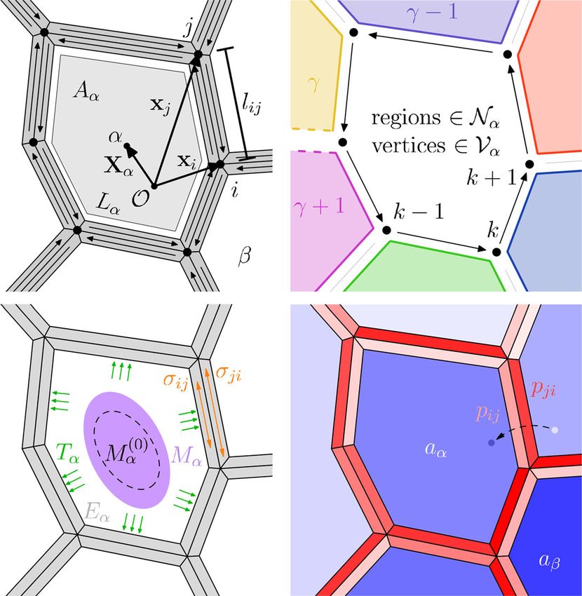
250   Page 2 of 22                                  Eur. Phys. J. Plus   (2021) 136:250

not limited to initiation of cell growth, cell division, and cell differentiation [12–14]. Estab-
lishment of auxin patterns is ubiquitous in plant organ morphogenesis [15]. The best char-
acterized example is the regular patterns of auxin spots in the outmost epidermal cell layer
at the tip of the shoot that prefigures the regular disposition of organs called phyllotactic
pattern [16–21]. These auxin accumulation spots mark the location of emerging primordia
of new aerial plant organs. Auxin patterns result from the polar distribution of auxin efflux
carriers called PIN-FORMED (PINs) [15,16,20,22–24]. Because of its prevalence in plant
development, understanding how these auxin patterns emerge has been intensively studied
and mathematically modelled. Auxin concentration feedback models [25–29], organize their
flow up-the-gradient of auxin concentration, reinforcing auxin maxima. Canalization models,
or flux-based models, [30–36] reinforce already existing flows, and, as such, both up-the-
gradient and down-the-gradient flows can exist. Some attempts at unifying both mechanisms
have been made [35,37–39], yet many conditions have to be imposed to explain, for instance,
the fountain-like patterns arising during root development [35,40].
    Tissue mechanics has emerged as a potent regulator of plant development [5,41–44]. Plant
cells are able to read mechanical stress and respond accordingly, rearranging their micro-
tubules along the main direction of mechanical stresses [41]. Furthermore, PIN1 polarity
and microtubules alignment at the shoot apical meristem are correlated [10], suggesting
the possibility of PIN localisation being mechanically regulated. This hypothetical coupling
between PIN localisation and mechanical cues is theoretically able to predict PIN polarity
and density for a wide range of cell wall stress and membrane tension [11]. Such coupling
is also supported by several other observations: the physical connection of PINs to the cell
wall [45], the change in polarity induced by cell curvature [46], and disorganization of PIN
polarity by modification of the cell wall mechanical properties [7].
    Auxin can induce remodelling of the cell wall and thus modify its mechanical properties
[4,6,7,47]. This may in turn influence PIN localisation and therefore have consequences on
the pattern of auxin. Modelling of this feedback in a tissue showed that mechanical stresses
can lead to the emergence of a regular phyllotactic auxin pattern by regulating PIN localisation
[10]. Although this result shows the importance of local mechanical coupling (Fig. 1) for
emergence of auxin patterns, the full extent of the impact of mechanical coupling on pattern
emergence remains unclear.
    In fact, cell strain is a compromise between its mechanical properties and the restrictions
placed upon its shape by the surrounding cells given the condition that the tissue remains
connected. In other words, stiffness variations contribute additional terms to tissue strain. In
order to explore the effect of the latter, we adapt the model for auxin transport introduced in
[10] to a vertex model mechanical description of the tissue, a tissue-wide mechanical model
and compare it to a uncoupled tissue approximation with the same auxin transport model but
where we prescribe an average stress acting on all cells (Fig. 2).
    By comparing both models, we find that due to stress fields arising from mechanical
feedback the magnitude of auxin spots is larger for lower stress-PIN coupling, indicating a
more efficient transition between low and high auxin regimes and the subsequent potential cell
behaviour response. Furthermore, we explore the information content of auxin distributions
when noise is considered and show that tissue-wide mechanical coupling improves robustness
of auxin patterns.

123
Eur. Phys. J. Plus      (2021) 136:250                                             Page 3 of 22      250

Fig. 1 Schematic representation of the cell–cell feedback mechanism between cell wall loosening via auxin
and mechanical control of PIN. (a) Auxin is transported to neighbouring cells via bound PIN efflux carriers.
(b) Auxin interacts with the mechanical properties of the cell wall reducing its stiffness. (c) Increasing stiffness
of a particular wall component shifts the stress load from the component of its neighbour to itself. (d) Wall
stress promotes PIN binding. A difference in auxin, therefore, induces a stress difference between the two
compartments separating both cells. This stress difference is such that PIN binds preferentially in the cell with
lower auxin concentration, increasing the flow of auxin into the cell with higher auxin concentration

Fig. 2 Schematic difference between the tissue-wide mechanical model (left) and the uncoupled tissue approx-
imation (right). In the tissue-wide mechanical model, turgor pressure, T , and stiffness determine the vertex
positions that minimize mechanical energy. Wall strain and stress are then inferred from the mechanical config-
uration. In the approximation, we prescribe average wall stress, σ̄ , with a static geometry. This approximation
disregards the effect of stiffness variations on strain. The prescription of stress in the approximation renders
the mechanical interaction to be only between nearest neighbours and uncoupled from all other cells. In the
tissue-wide mechanical model, the mechanical state is a function of all cells in the tissue

2 Methods

In order to investigate the interaction between auxin cell wall softening and collective tissue
mechanics, we use a vertex model to describe the mechanical behaviour of the tissue and a
compartment model to express auxin concentration and transport between adjacent cells.

                                                                                                      123
250    Page 4 of 22                                         Eur. Phys. J. Plus      (2021) 136:250

Fig. 3 Vertex model description of a cell as a geometrical, mechanical, and biologically active entity. (top
left) A cell α surrounded by its cell walls with centroid Xα , area Aα and perimeter L α . Vertices i and j
have positions xi and x j and the distance between them is li j = l ji . (top right) Set of surrounding regions,
one for each wall, Nα , and set surrounding vertices, Vα , used in the equations of the model. (bottom left)
Mechanically, cell α is under turgor pressure Tα , the surrounding wall compartments have stiffness E α . Mα is
                                                   (0)
the second moment of area of cell α, whereas Mα is that same quantity when the cell is at rest. σi j refers to
the longitudinal stress acting on the compartment of the wall. (bottom right) Cell α has an auxin concentration
aα which is expressed, degraded and transported, both passively and actively. The active component of auxin
transport relies on the density of membrane-bound efflux auxin carriers facing a particular wall compartment,
pi j

2.1 Geometrical set-up of the tissue

The tissue is described by a tiling of two-dimensional space into M cells surrounded by
their cell walls. Walls are represented as edges connecting two vertices each, positioned at
xi = (xi , yi ) , i ∈ [1, N ]. Here, we reserve Latin indices for vertex numbering and Greek
ones for cells. Each cell wall segment has two compartments, one facing each cell. Therefore,
we represent each cell wall with two edges of opposite direction, one for each compartment.
The position of tissue vertices fully define geometrical quantities such as cell areas, Aα , cell
perimeters, L α , wall lengths, li j = l ji , and cell centroids, Xα (Fig. 3 top left). To simplify
notation significantly, we also define for each cell the cyclically ordered   set of all vertices
around that cell, Vα , arranged counterclockwise (ccw). Hence, we use i∈Vα to signify the
sum over all vertices surrounding cell α with an arbitrary start, where i + 1 and i − 1 mean,
respectively, the next and previous ccw vertex. Similarly, we introduce Nα as the cyclically
ordered (counterclockwise) set of all neighbouring regions around cell α, one for each edge
of α (Fig. 3 top right).

123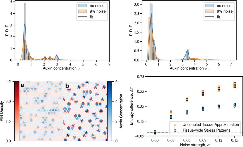
Eur. Phys. J. Plus   (2021) 136:250                                     Page 5 of 22   250

2.2 Tissue mechanics–tissue-wide coupling

Vertex models are a widely employed theoretical approach to describe mechanics of epithelial
tissues and morphogenesis [9,48–53]. The essence of vertex models is that cell geometry
within a tissue is given as the mechanical equilibrium of the tissue. In the case of plant cells,
the shape of a cell is a competition between the turgor pressure, Tα , all cells exert on each
other and the cell’s resistance to deformation with stiffness, E α . Strain acting on each cell
will be described using the second moment of area of the corresponding cell in reference to
its centroid, Mα , whose components are
                         ni  2
              Mα x x =           xi + xi xi+1
                                                    2
                                                  + xi+1    ,                                (1)
                             12
                       i∈Vα
                         ni  2
              Mα yy =            yi + yi yi+1
                                                    2
                                                  + yi+1   ,                                 (2)
                             12
                       i∈Vα
                                  ni
              Mαx y = Mα yx =              xi yi+1

                                                    + 2xi yi + 2xi+1

                                                                       yi+1
                                                                            + xi+1 yi ,     (3)
                                     24
                                 i∈Vα

where the primed coordinates represent the translation transformation, xi = xi , yi =
xi − Xα , and n i = xi yi+1
                                y  , i ∈ V . Given a rest shape matrix, M (0) , we define cell
                             − xi+1 i        α                              α
strain as the normalized difference between both matrices,
                                                        (0)
                                               Mα − Mα
                                        εα =           ,                                      (4)
                                                    (0)
                                               Tr Mα

and stress with σα = E α εα . Having described the tissue mechanically (Fig. 3 bottom left),
we define the energy for a single cell as the sum of work done by turgor pressure and elastic
deformation energy, resulting in the tissue mechanical energy,
                                ⎡                                    ⎤
                                                      (0) 2
                             ⎢1
                             M                M α − M α
                                                                     ⎥
                      H=        ⎣ Aα E α                 2 − Aα Tα ⎦ .                  (5)
                                  2              2 M (0)
                            α=1               Tr     α

Using this model, we obtain the shape of the tissue by minimizing H with respect to vertex
positions.
   After minimizing (Eq. 5), we quantify the stress acting on each wall through the average
strain acting on each cell given by (Eq. 4). Assuming that cell wall rest length is the same
between two adjacent wall compartments then it follows that they are under the same longi-
tudinal strain, which is, to first approximation, the average between the two cells surrounding
them. Therefore, longitudinal average strain acting on a specific wall used here is
                                                    εα + εβ
                                 ε̄αβ = ε̄βα ∼ t̂αβ
                                                 T
                                                             t̂αβ ,                              (6)
                                                        2
where tαβ is a unit vector along the wall separating cell α and cell β. Note that this interpolation
assumes a continuous strain field. Then the stresses acting on each compartment are by the
constitutive equation of a linear elastic isotropic material with Poisson ratio ν = 0,
                                σαβ = E α ε̄αβ  = σβα = E β ε̄βα .                             (7)
Note that we are only considering the longitudinal components with regards to the cell wall,
which means that ε̄αβ and σαβ are scalar quantities. More details on the mechanical model

                                                                                        123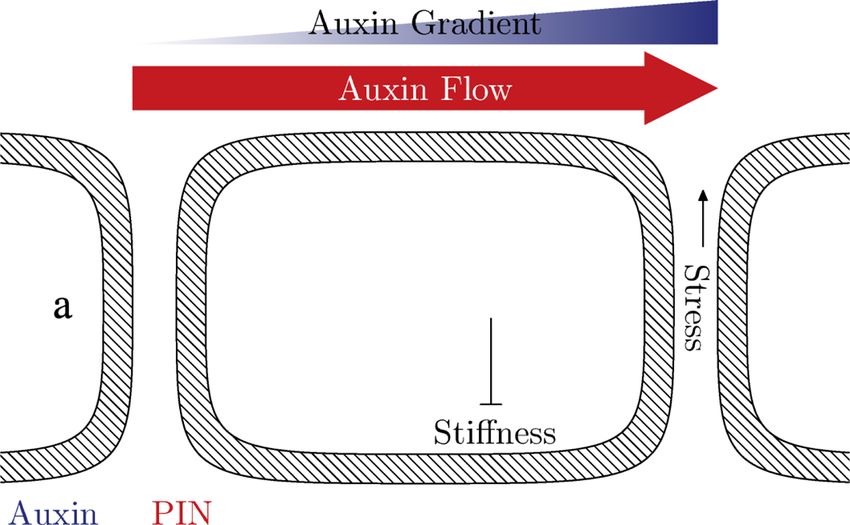
250   Page 6 of 22                                   Eur. Phys. J. Plus   (2021) 136:250

used can be found in the supporting text. As argued in the supporting material, our choice of
ν = 0 does not impact the qualitative behaviour studied here.

2.3 Tissue mechanics–uncoupled tissue approximation

To assess the impact of collective mechanical behaviour within a tissue on auxin pattern self-
organization, we approximate the tissue-wide mechanical model to a static tissue geometry
where we approximate the effects of turgor pressure of each individual cells in the static tissue
by a constant average stress σ̄ acting on it [10]. Again assuming that both wall compartments
have the same rest length, we infer that the stress acting on a particular wall depends only on
σ̄ and the stiffness of the adjacent cells. Effectively, the average longitudinal strain acting on
a wall surrounded by cells α and β would simply be

                                 ε̄αβ = ε̄βα = 2σ̄ / E α + E β .                               (8)

This way, instead of minimizing the full mechanical model (Eq. 5) given a set of turgor
                                       (0)
pressures Tα and rest shape matrices Mα we can, in the static tissue, immediately compute
stress with Eq. 7 yielding,
                                            2E α σ̄
                                     σαβ =          .                                 (9)
                                           Eα + Eβ
Interestingly, Eq. 9 is valid for ν  = 0 as demonstrated in the supporting material.
   In order to compare the two models, we choose the value of σ̄ to be the same as the stress
                                                                         (0)
obtained through minimisation of (Eq. 5), for a given set of Tα and Mα , with the constraint
of the same end geometry.
   Note that not only can this approximation be interpreted as the tissue being mechanically
coupled only to the nearest neighbours, disregarding the rest of the tissue, (Fig. 2), but also
as an analogous non-mechanical auxin concentration feedback model.

2.4 Auxin transport–compartment model

Compartment models for auxin transport are well adapted to the context of plant development,
since the prerequisite of a boundary of a plant cell is particularly well defined by courtesy of
the cell wall.
   Although passive diffusion occurs across cell walls, the dominant players in auxin transport
are membrane-bound carriers [22,24]. Namely, efflux transporters of the PIN family are
important due to their anisotropic positioning around a cell [16], which leads to a net auxin
flow from one cell to the next. Let aα denote an non-dimensional and normalized average
auxin concentration inside cell α. Following the model by [10], which is similar to previous
mathematical models [25,26,29], auxin evolves according to auxin metabolism in the cell,
passive diffusion between cells and active transport across cell walls via PIN,
                      daα
                          = γ ∗ − δ ∗ aα + D      Wαβ aβ − aα
                       dt
                                             β∈Nα

                                                   aβ            aα
                            +P         Wαβ pβα          − pαβ           ,                    (10)
                                                 K + aβ        K + aα
                                 β∈Nα

where γ ∗ is the auxin production rate, δ ∗ is the auxin decay rate, Wαβ = lαβ /Aα , with K ,
P , and D as adjustable parameters. D is the passive permeability of plant cells, whereas P is
permeability of the cell wall due to PIN-mediated transport of auxin, and K is the Michaelis–

123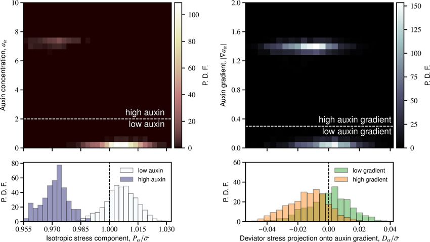
Eur. Phys. J. Plus   (2021) 136:250                                           Page 7 of 22   250

Menten constant for the efflux of auxin. More information on how this expression is derived
can be found in the supporting text. Although this description ignores the auxin present within
the extracellular domain and inside the cell wall, it has been shown that under physiological
assumptions, this is a valid approximation [29]. The active transport term depends on the
amount of bound PIN in each cell wall,
                                                f αβ
                              pαβ =                lαγ
                                                                 , β ∈ Nα ,                        (11)
                                      1+      γ ∈Nα L α   f αγ

where f αβ , β ∈ Nα expresses the ratio between binding and unbinding rates of a particular
wall (Fig. 3 bottom right). Note that pαβ is different from wall to wall and from cell to cell.
This means that in general, pαβ  = pβα , or equivalently, pi j  = p ji . This is consistent with the
fact that there are two compartments to a cell wall shared by two adjacent cells. Expression
(Eq. 11) is based on the assumption that cell walls around a particular cell compete for the
same pool of PIN molecules and that the amount of PIN scales with cell perimeter. This
competition has been shown to be important in the polarization of PIN [29]. Alternatively,
one could also scale the amount of PIN with cell size or not scale it at all. In the former case,
smaller cells would be slightly preferred for auxin accumulation, whereas in the latter, larger
cells would be preferred instead. Since we want to study the impact of stress patterns on the
tissue, we want to decouple it from this effect as much as possible, choosing instead to scale
the amount of PIN with perimeter.
    The trivial fixed point of these dynamical equations is given by aα = μ∗ /δ ∗ , ∀α, which
also results in equal PIN density across all walls, provided turgor pressure Tα and stiffness
E α are the same across the tissue.
    The feedback between tissue mechanics and auxin pattern unfolds as auxin transport
affects tissue mechanics due to auxin, aα , controlling cell wall stiffness, E α , and in reverse
tissue stress, σα , affects auxin transport by regulating PIN binding rates, f αβ , as hypothesized
by [10,11].

2.5 Mechanical regulation of PIN binding

According to the hypothesis presented by [10,11], mechanical cues up-regulate PIN binding.
The distinction between whether these mechanical cues are strain or stress has been studied
recently by [54], yet the exact nature remains unclear. Following the model presented by
[10], we model the binding-unbinding ratio, f αβ , as being a power law on positive stress,
                                             n
                                          η σαβ , σαβ > 0,
                          f αβ = f σαβ =                                                 (12)
                                            0,            σαβ ≤ 0,

where the stresses, σαβ , follow from tissue mechanics after minimization of the full mechan-
ical model (Eq. 5), or, in the averaged stress approximation, it is the stress load on that
particular compartment given by (Eq. 9). Furthermore, n is the exponent of this power law,
and η captures the coupling between stress and PIN. Effectively, this mechanical coupling to
PIN parameter corresponds to the sensing and subsequent response to stress, loosely trans-
lating into how much resources the cell needs to spend for processing stress cues.

2.6 Auxin-mediated cell wall softening

Auxin affects the mechanical properties of a cell wall via methyl esterification of pectin
[6,7], resulting in a decrease of the stiffness of the cell wall. We assume that all cell wall

                                                                                              123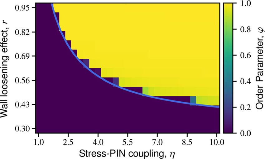
250    Page 8 of 22                                          Eur. Phys. J. Plus      (2021) 136:250

Fig. 4 Schematic representation of the time evolution of the model. From mechanical relaxation of the
mechanical model, we calculate PIN densities on each wall via stress. Then we integrate auxin dynamics for a
time step and update the stiffness of each cell. This process knocks the system out of the previous mechanical
energy minimum, and it has to be relaxed again. Alternatively, we can shortcut energy minimization using the
averaged stress approximation for a static tissue. This procedure is repeated until t = tmax . The parameters r ,
wall loosening effect, and η, stress coupling, interface both models and are, therefore, of critical importance
to the mechanism studied

compartments surrounding cell α share the same stiffness, E α . To capture this effect, we
model stiffness with a Hill function [10],

                                                      1 − aαm
                            E α = E (aα ) = E 0 1 + r           ,                     (13)
                                                      1 + aαm
where r ∈ [0, 1[ which we define as the cell wall loosening effect, m is the Hill exponent
of this interaction, and E 0 is the stiffness of the cell walls when its auxin concentration is
aα = 1. At low values of auxin, E α approaches the value (1 + r ) E 0 , whereas at high auxin
concentration, E α approaches (1 − r ) E 0 . Given a distribution of auxin, we can compute
the wall stiffness in (Eq. 5) from (Eq. 13), or the stress acting on a specific compartment in
(Eq. 9) for the approximated model.

2.7 Integrating auxin transport and tissue mechanics

At each time step, Δt, starting from an auxin distribution, we compute the stiffness of each
cell according to (Eq. 13). Then, with the input of all turgor pressures, we minimize (Eq. 5)
to obtain tissue geometry and stresses acting on each wall. Auxin concentration in each cell
will evolve according to (Eq. 10), where the active transport term will be regulated by stress
according to (Eq. 12) via (Eq. 11). A new auxin distribution will result at the end of this
iteration, and we will be ready to take another time step (Fig. 4). We repeat this process until
t = tmax .

2.8 Implementation

We implemented this model with C++ programming language, where we have used the
Quad-Edge data structure for geometry and topology of the tissue [55], implemented in
the library Quad-Edge [56]. In order to minimize the mechanical energy of the tissue, we
have used a limited-memory Broyden–Fletcher–Goldfarb–Shanno algorithm (L-BFGS) [57,
58], implemented in the library NLopt [59]. For solving the set of ODEs presented in the

123
Eur. Phys. J. Plus (2021) 136:250 Page 9 of 22 250
compartment model, we used the explicit embedded Runge–Kutta–Fehlberg method (often
referred to as RKF45) implemented in the GNU Scientific Library (GSL) [60]. We wrapped
the resulting classes into a python module with SWIG. For additional details regarding
the parameters used for the simulations of the following section, consult Table S1 in the
supporting material.
2.9 Observables
In order to quantify the existence of auxin patterns, we compute the difference between an
emerging auxin concentration pattern and the trivial steady state of uniform auxin concentra-
tion pattern defined as aα = γ ∗ /δ ∗ , ∀α. To account for a large range of orders of magnitude
of auxin concentration, we consider as an order parameter,
2
ln (aα ) M
ϕ= 2 2 , (14)
δ + ln (aα ) M
where · M denotes an average over all cells within the tissue. This way, ϕ ≈ 0 means that
there are no discernible patterns, whereas ϕ ≈ 1 implies prominent auxin patterning. The
term δ 2 defines the sensitivity of this measure, such that an average deviation of δ yields
ϕ ≈ 1/2 (for small δ). We will choose δ = 0.1, i. e. , a 10% deviation from the trivial steady
state.
We also keep track of the average of auxin above basal levels in order to gauge the potential
degree of modulation of auxin-mediated cell behaviour.
Furthermore, to characterize cells with regards to PIN localization we introduce the mag-
nitude of the average PIN efflux direction,
lii+1
Fα = pii+1 n̂ii+1 , (15)
Lα
i∈Vα
where n̂ii+1 is the unit vector normal to the wall pointing outwards from α.
Aside from a global measure of auxin patterning, it is also important to locally relate
auxin to tissue mechanics. Namely, for auxin we are interested in auxin concentration, aα ,
and auxin local gradient, obtained by interpolation,
1 Yγ +1 −Yγ aγ − aα
∇aα = , (16)
2 A∗α −X γ +1 X γ aγ +1 − aα
γ ∈Nα
where Xγ = X γ , Yγ = Xγ − Xα and
1
A∗α = X γ Yγ +1 − Yγ X γ +1 . (17)
2
γ ∈Nα
In fact, the quantity |∇aα | can be used as an indicator of whether there is an interface between
auxin spots and the rest of the tissue.
With regards to tissue mechanics, the local quantities we quantify are the isotropic com-
ponent of stress,
1
Pα = Tr (σα ) , (18)
2
123250 Page 10 of 22 Eur. Phys. J. Plus (2021) 136:250
and the stress deviator tensor projected along the direction of the auxin gradient,
∇aαT σα ∇aα
Dα = , (19)
|∇aα |2
where σα = σα − I Pα , and I is the identity matrix. Therefore, Pα is a measure if a cell is
being compressed (Pα < 0), or pulled apart (Pα > 0), and Dα translates into if a cell is
more compressed along the auxin gradient than perpendicular to it (Dα < 0), or vice-versa
(Dα > 0).
Finally, to measure the disruption of an auxin pattern we approximate entropy by means
of a Riemann sum,
∞
S [Π] = − Π (iΔa) Δa ln (Π (iΔa) Δa) , (20)
i=−∞
where Π (a) is the probability density function of auxin and Δa the partition size. Note that
it is only meaningful to compare entropy measures obtained with the same partition size
Δa. Here, the probability density function of auxin concentration is obtained by applying a
kernel density estimation on the resulting tissue auxin values. Note that Π (a) is a continuous
function. In order to infer it from simulation
∞ data, for each auxin value in the tissue, aα , we
add Kernel functions K w (a), obeying −∞ K w (a)da = 1 and K w (a) = K w (−a). Then we
can estimate
1
M
Π (a) ∼ K w (a − aα ), (21)
M
α=1
where w is a smoothing parameter defining the width of the Kernel, this parameter is some-
times called bandwidth. This statistical tool is called kernel density estimation (KDE) [61].
We use the Epanechnikov kernel because it is bounded and we can force Π (a) = 0, a ≤ 0.
3 Results
3.1 The tissue-wide mechanical model captures stress patterns after ablation
First we verify that the tissue-wide mechanical model captures the expected mechanical
behaviour and auxin patterning when a cell is ablated. To model ablation, we set the stiffness
of the ablated cell walls to E 0 = 0, block all auxin transport to and from it, block PIN
transporters of adjacent cells from binding to the shared wall with the ablated cell, and,
finally, we lower the turgor pressure to only 10% of the original value. This remnant of
pressure represents the surface tension emerging from pressure of the inner layers of the shoot
apical meristem acting on a curved surface, as required by the Young–Laplace equation. This
is necessary since the model only simulates the epidermal layer in a plane.
We observe that the region neighbouring the ablation site gets depleted of auxin due to
PIN binding preferentially to the walls circumferentially aligned around the ablated cell in
accordance with the stress principal directions (Fig. 5a). This stress pattern is in agreement
with calculations performed by [41] in this setting and PIN aligns according to the ablation
experiments in [10].
We also simulated different wound shapes. The resulting stress patterns are shown the
supporting material. Stress directions align along the shape of the ablation wound.
123Eur. Phys. J. Plus (2021) 136:250 Page 11 of 22 250
Fig. 5 Tissue-wide mechanical model captures expected stress patterns as well as auxin and PIN distribution
λ −λ
after ablation. Green lines represent the magnitude and direction of principal stress, measured γ = λ+ +λ− ,
+ −
where λ± are the largest and lowest eigenvalues of the stress tensor. The ablation perturbs auxin patterning by
redirecting PIN. This PIN reorientation coincides with the circumferential stress patterns around the ablation
site, as seen in experiments and simulations [10,41].r = 0.65 and η = 1.5
Fig. 6 Simulation results of the order parameter ϕ, indicator for the existence of auxin patterns, as a function
of r ∈ [0.30, 0.95] and η ∈ [1.0, 10.0] for a model with tissue-wide stress patterning. The simulated tissue is
composed of 2977 initially hexagonal cells. The blue line represents the analytically predicted instability for
the uncoupled tissue approximation (Eq. 22)
Thus our mechanical model faithfully capture the typical tissue behaviour upon ablation
with regards to stress, auxin and PIN transporter patterns.
3.2 Conditions for auxin patterns emergence
The uncoupled tissue approximation allows to analytically compute the conditions for spon-
taneous auxin pattern emergence in a general regular lattice (Fig. 6). Effectively, for a regular
grid, the condition for pattern formation is,
2
K +1 PK D
M> 1 + 1 + 2W + , (22)
WP (K + 1)2 p0
123250 Page 12 of 22 Eur. Phys. J. Plus (2021) 136:250
√
where M = nmr , W = 4/ 3 is a geometrical factor specific to the used grid, and p0 =
f (σ̄ ) /(1 + f (σ̄ )) (see supporting material for the linear stability analysis details). Equation
22 is the closed form of more general expressions presented by [10,29] tailored to our system
and parameters.
To quantify the existence of auxin patterns in the model with tissue-wide stress patterning,
we computed the order parameter ϕ defined in Eq. 14 for simulations with different values of
wall loosening effect r and stress coupling η (Fig. 6). These two parameters are conceptually
important since the former is the cause for stiffness inhomogeneity of the tissue, and the
latter represents a plant cell’s sensitivity to mechanical cues.
We observe a very good agreement between the conditions for pattern emergence (Eq. 22)
analytically predicted in the case of the uncoupled tissue approximation and the transition
of ϕ in the case of tissue-wide stress patterning (Fig. 6). This means that at the onset of
patterns emergence the auxin concentrations are similar enough to make the assumption that
the effect of turgor pressure is simply an isotropic stress across the entire tissue, validating
the approximation near the transition. This observation is in agreement with the auxin pattern
emergence mechanism hypothesis by [10] (Fig. 1). The agreement between the two models
does not necessarily apply after patterns emerge. This poses the question of the role of
mechanics in potentially enhancing or hindering auxin flows.
3.3 Global mechanical response reinforces PIN polarity
To understand the role of tissue-wide stress patterning on the emergence of PIN-driven auxin
patterns, we quantify how PIN rearranges in the model with tissue-wide stress patterning
ver sus the uncoupled tissue approximation.
We compute the average PIN efflux direction, i.e., average PIN polarity for each combina-
tion of the parameters r (auxin-induced cell wall loosening) and η (coupling of PIN to stress)
under the approximated (Fig. 7 top left) and tissue-wide (Fig. 7 top right) stress coupling
regimes.
We observe an overall increase in PIN polarity in the tissue-wide stress coupling regime
compared with the uncoupled tissue approximation. PIN polarity also becomes more sen-
sitive to r . For very low values of r , tissue stress patterns are slightly detrimental to auxin
patterning. These data show that saturation of PIN polarity happens earlier with respect to η
for intermediate values of r . For high values of r , we observe a non-monotonic dependence
of polarity on η, effectively translating into an optimal value of η.
Visual inspection of the simulations results reveals higher PIN density in proximity of
auxin spots and an increase in magnitude of these auxin peaks upon tissue-wide stress pat-
terning (Fig. 7a–d). Moreover, we observe a severe alteration of pattern size and wavelength
between both models (Fig. 7 bottom left).
These results show that tissue-wide stress patterning reinforces PIN polarity and that auxin
spots are sharper. Next we will quantify how much sharper these auxin spots become.
3.4 Tissue-wide coupling induces efficient emergence of auxin spots
Auxin levels in the shoot apical meristem have been shown to affect cell fate reliably [20],
even if the flexibility of the auxin signalling mechanism allows for many potential outcomes
[62]. We explore auxin spot concentration achieved by both models in order to gauge the
impact of tissue-wide stress patterns on the distinguishability of primordium cells.
For this, we first characterize quantitatively the auxin spot average concentration measured
for each simulation of the uncoupled tissue approximation (Fig. 8 left) and tissue-wide
123Eur. Phys. J. Plus (2021) 136:250 Page 13 of 22 250
Fig. 7 Quantification of PIN polarity in both models reveals more focused auxin spots due to tissue-wide
integration via mechanical coupling. (top) Average magnitude of PIN polarity, Fα M , as a function of stress-
PIN coupling, η, and wall loosening effect, r , for (top left) the uncoupled tissue approximation and (top right)
for the tissue-wide stress patterning. PIN polarity magnitude increases when considering the mechanics of
the whole tissue, with a particularly strong dependence on the wall loosening affect r of auxin. The labels
represent the parameters plotted for (a, b, c, d) comparison between example results of auxin concentration
and PIN density of simulations using the uncoupled tissue approximation (a, c) and the tissue-wide stress
patterning (b, d), for the same value of η = 5.5, and r = 0.65 (bottom left) or r = 0.90 (bottom right). In both
instances, we observe that PIN polarity and auxin concentration are higher upon tissue-wide stress patterning
(b, d)
Fig. 8 Characterization of auxin spot concentration reveals more focused auxin spots due to tissue-wide
integration via mechanical coupling. Average auxin concentration for cells above basal auxin concentration
(aα > 1), for the uncoupled tissue approximation (left), and upon tissue-wide stress patterning (right), as a
function of stress-PIN coupling, η, and wall loosening effect, r . Spot auxin concentration increases with both
η and r in (left); however, in (right), it increases predominantly with r . For medium to high values of r , auxin
concentration jumps to several times immediately after emergence
stress coupling (Fig. 8 right) regimes. We use, as a proxy, the average of cells with auxin
concentration aα > 1 to identify auxin spots.
We observe that the dependence on the parameter r recognized for PIN polarity translates
into auxin spot concentration. For medium to high values of r , auxin concentration is several
123250 Page 14 of 22 Eur. Phys. J. Plus (2021) 136:250
Fig. 9 Map of auxin distribution and PIN density aligns with stress direction. Green lines represent principal
λ −λ
direction of stress, measured as γ = λ+ +λ− , where λ± are the largest and lowest eigenvalues of the stress
+ −
tensor. We observe that stress directions in part congruent with auxin spots. r = 0.90 and η = 5.5
times higher when accounting for tissue-wide behaviour than when considering the uncoupled
tissue approximation.
Additionally, at the onset of pattern formation for medium to high values of r , we observe
a considerable jump in average auxin spot concentration for a small change in η. This increase
in sensitivity to a change in η of the system, under the aforementioned conditions, implies a
boost in mechanosensing capabilities when considering tissue-wide stress patterning.
Our results point to stress patterns being responsible for the enhancement of auxin spot
concentration and flows. In order to make sure we understand why, we decided to observe
and quantify stress patterns and their connection to auxin distribution.
3.5 Part of wall stress within spots is borne by walls at the interface
In order to analyse tissue-wide stress patterns, we choose an example that has simple auxin
patterns that allow for a straightforward interpretation. Under this condition, we choose the
parameters r = 0.90 and η = 5.5 already presented in Fig. 7d, for which we plot on it a
measure of anisotropy along the largest principal stress direction (Fig. 9). Here it becomes
apparent that stress patterns are related, even if not absolutely, to auxin spot patterns.
To explore this further, we quantify several local quantities, such as auxin concentration,
aα , auxin gradient norm (Eq. 16), |∇aα |, isotropic stress component (Eq. 18), Pα , and deviator
stress tensor projection onto auxin gradient (Eq. 19), Dα . For the example mentioned above,
we record the histograms of the simultaneous occurrence of the pairs (aα , Pα ) (Fig. 10 top
left) and (|∇aα | , Dα ) (Fig. 10 top right).
We can section the results according to high or low auxin concentration (Fig. 10 bottom
left), and high or low auxin gradient (Fig. 10 bottom right). Here, high auxin cells are a proxy
for auxin spot cells, and high auxin gradient cells are a proxy for cells neighbouring auxin
spots. Taking into account that in the uncoupled tissue approximation Pα = σ̄ and Dα = 0
by construction, we can get a better picture of tissue-wide stress patterns.
We observe from data (Fig. 10 bottom left) that Pα in cells of auxin spots is lower than
in the uncoupled tissue approximation and accompanied by a slight shift in the opposite
direction of the Pα of the remaining cells. Additionally, we register a noticeable shift towards
negative Dα for high auxin gradient cells (Fig. 10 bottom right).
123Eur. Phys. J. Plus (2021) 136:250 Page 15 of 22 250
Fig. 10 Stress pattern self-organization concomitant with auxin patterns. Probability density functions
(P.D.F.s) of (top left) auxin concentration and isotropic stress component and (top right) auxin gradient magni-
tude and deviator stress tensor projection onto auxin gradient. In each case, we can identify two populations of
cells: high and low auxin concentration (bottom left), and high and low auxin gradient (bottom right). (bottom
left), since Pα = σ̄ signifies the stress that would be expected in the uncoupled tissue approximation, high
auxin concentration cell expansion is constrained by the remaining cells which are, in turn, under a larger
amount of stress. On the other hand (bottom right) we observe that the auxin spot neighbours have, on average,
negative values of Dα , indicating that the largest principal stress direction is perpendicular to auxin gradients,
i.e., circumferentially aligned around auxin spots, as suggested by Fig. 9. r = 0.90 and η = 5.5
Taken together, these data suggests that cell walls at the interface of a spot are under a
larger amount of stress whereas the cells within auxin spots have decreased stress. This leads
to reinforced polar auxin transport towards the spot and hence higher auxin concentration.
The lower isotropic stress component inside the auxin spot suggests that the diffusive term
inside auxin spots increases in importance relative to the active transport term.
3.6 Tissue-wide stress coupling mitigates disruption by noise
Up until now, our simulations were performed on hexagonal tissues in the absence of noise.
This also raises the question of how tissue-wide stress patterns impact pattern emergence
robustness against noise.
In plant tissue as any biological entity, noise prevails. As such cells within a tissue differ
in their mechanical parameters. In order to inspect how parameter noise disrupts pattern
emergence, we choose to sample reference stiffness, E 0 , from a normal distribution for each
cell. As outlined in the supplementary material, we expect this parameter to be the most
disruptive to the active term and it is reasonable to assume it changes from cell to cell. We
then simulate the resulting tissue with the uncoupled tissue approximation and tissue-wide
stress coupling.
We simulate tissues with r = 0.65 and η = 5.5 for both models by promoting E 0 to a
random variable sampled from Gaussian distribution with mean E¯0 = 300 MPa and standard
deviation of α E¯0 , α ∈ {0.03, 0.06, 0.09, 0.12, 0.15}, where α is the noise strength. For each
value of α, five simulations were performed per model. We fit the resulting auxin distributions
123250 Page 16 of 22 Eur. Phys. J. Plus (2021) 136:250
Fig. 11 Impact of noise in reference stiffness in the auxin concentration distributions for the uncoupled
tissue approximation and upon tissue-wide coupling reveals robustness of auxin patterns due to tissue-wide
integration. For a given noise strength, auxin concentration probability density functions (P.D.F.s) are extracted
from simulation results by means of a kernel density estimation for the uncoupled tissue approximation (top
left) and when considering tissue-wide stress patterns (top right). The simulated tissues have r = 0.65 and
η = 5.5. For both models, we observe broadening of the distributions when considering noise. In each instance,
the fit appears to be adequate for describing the resulting auxin concentration. (bottom left) Examples of the
resulting patterns in the uncoupled tissue approximation (a) and in the case of tissue-wide stress patterns (b)
for a noise strength of 9%. Even though patterns are heavily disrupted, we can still discern more clearly high
auxin concentration spikes upon tissue-wide coupling. (bottom right) Entropy difference between the resulting
distributions for a given noise strength and in the absence of noise. In the presence of tissue-wide stress patterns
disruption of tissue patterning is consistently lower than in the uncoupled tissue approximation
to a probability density function (Fig. 11 top left and top right). We observe that noise in
reference stiffness impacts the patterning behaviour in a severe manner (Fig. 11 bottom left).
Yet, with tissue-wide stress coupling spots of noticeable auxin accumulation are preserved.
In order to quantify the disruption, we compute the entropy (Eq. 20) of a fitted auxin
probability density function by means of a kernel density estimation on the resulting auxin
distributions. The kernel used for all fits was the Epanechnikov kernel with a bandwidth
of about 0.202. This number arises in the rule-of-thumb estimate for the Gaussian kernel
for the sample size and dimension of this system. The partition size used for the numerical
approximation of the entropy is the same for all instances. Afterwards, we measure the entropy
difference between the expected auxin distribution for each value of α, of each model and for
all simulations (Fig. 11 bottom right). The reference entropy is taken to be the average of the
uncoupled tissue approximation at α = 0. We can infer from these results that tissue-wide
coupling helps to rescue auxin accumulation spots despite its heavy disruption in comparison
to the uncoupled tissue approximation.
3.7 High turgor preferred but not required for sustaining auxin maxima
It is of interest to the experimental community at this point in time how auxin spots
and turgor pressure correlates [63,64]. To explore how the the tissue-wide mechanical model
123Eur. Phys. J. Plus (2021) 136:250 Page 17 of 22 250
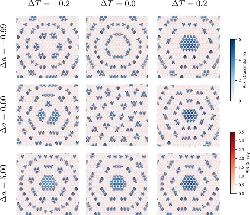
Fig. 12 Simulations of auxin patterning with the tissue-wide mechanical model when considering a local
turgor increase (right column), decrease (left column), or constant (middle column), and a prior high (bottom
row), low (top row), or constant (middle row) initial auxin concentration. Units of ΔT are MPa. We used
η = 10 and r = 0.65 for all simulations. Even if high turgor predicts an auxin maximum, it becomes unclear
what might happen with low turgor. The tissue-wide mechanical model seems to preserve already existing
auxin maxima
responds to local turgor variations, we probe what happens when patterns emerge with a local
increase or decrease in turgor. Since stress is tied to active auxin flow, the results are prone to be
affected by prior auxin concentration distribution. Hence, we test the several turgor scenarios
x 2 +y 2
as well as initial auxin concentration. We added a contribution to turgor of ΔT e− 2σ , where
ΔT ∈ {−0.2, 0.0, 0.2} MPa and σ = 2L. For initial auxin concentration, we used the same
form with the same σ , yet the largest deviations are Δa ∈ {−0.99, 0.00, 5.00}. To be sure
we are well within the pattern formation regime of the model for low pressure, we used the
stress-PIN coupling value of η = 10 and r = 0.65.
Regardless of initial auxin concentration, for high turgor, we observe an auxin maximum
predictably emerges correlated with a turgor maximum (Fig. 12 right column). Nevertheless,
if an initial auxin concentration exists, we also predict that the spot remains regardless of
whether this position is a turgor minimum or not (Fig. 12 bottom row). Low turgor regions
can still exhibit patterns adding to the complexity of this simple measure (Fig. 12 middle
row, left).
From these data, we can conclude is that developmental history is as important as turgor
pressure for predicting auxin maxima positioning. We can predict high turgor leads to auxin
123250 Page 18 of 22 Eur. Phys. J. Plus (2021) 136:250
accumulation, yet low turgor gives us little insight on auxin distribution. We can also predict
that a high auxin concentration region.
4 Discussion
Here, we used a model composed of a vertex model for plant tissue mechanics, and a com-
partment model for auxin transport to uncover the role of tissue-wide mechanical coupling
on auxin redistribution. We first verified that the tissue-wide mechanical model successfully
captures the behaviour of plant tissue upon ablation experiments and the conditions for emer-
gence of auxin patterns. We then compared the behaviour of our model featuring tissue-wide
mechanical coupling to an approximation which regards cells as mechanically isolated. We
observe the emergence of focused auxin spots with high auxin concentration when tissue-
wide mechanical coupling is implemented. Notably, depending on the parameters of the
tissue-wide stress model, auxin spot concentration is more sensitive to stress than what could
be predicted from the approximation. We observe that tissue-wide mechanical effects unac-
counted for by the approximation have a positive impact on PIN polarity. Furthermore, we
show that stress patterning of the tissue mitigates the disruption caused by noise, increas-
ing robustness of the system. Finally, we observe auxin concentration correlating with high
local turgor pressure. This behaviour coexists with the possibility of having auxin maxima
anti-correlating with turgor.
The auxin-induced cell wall loosening effect (r parameter in this work) is an important
determinant of the feedback of auxin on tissue mechanics. The range of values of r for
which substantial pattern focusing occurs is around r ∼ 0.60 and above in our model. This
translates into a variation of stiffness from a minimum value E min up to E max = 4E min
(see supplementary material). Although high, this range is within biological expectation and
supported by AFM measurements on auxin treated tissues [7] and comparable to previous
simulations of this mechanism [10] where E max /E min = 5 which translates into r = 2/3.
Comparison of the tissue-wide stress patterning case to the uncoupled tissue approximation
reveals that auxin spot concentration has a very steep transition in the former case (Fig. 8).
This results in a several-fold increase in auxin concentration at values of η close to the
threshold for pattern formation. What was once a relatively subtle graded response of auxin
spot concentration on stress behaves now as an on-off switch by virtue of tissue mechanical
relaxation. Since the mechanical perturbations being highlighted through the comparison are
purely passive, this improvement in sensing comes at no additional cost for the plant and
therefore has the potential to increase efficiency.
In the present work, we explored the parameter space (η, r ) exclusively. We observe
consistently that pattern wavelengths shorten from the uncoupled tissue approximation and
the tissue-wide coupling model. It would be interesting to systematically probe the diversity
of patterns and how they change upon tissue-wide mechanical coupling. For our simulations,
we used the parameters n, m, K from [10], parameters on which we have little empirical
information. Yet, the sensitivity analysis from [29] suggests that n and K especially should
affect patterning the most. We speculate the parameter m, specific to wall loosening, to be of
similar importance. We expect that a study focusing on these three parameters would yield
more interesting patterns shapes.
This work focused exclusively in the hypothesis that PIN is mechanically regulated. How-
ever, competing chemical feedback mechanisms have been proposed. Recently, mechanics
and ARF-mediated PIN expression have been modelled together by [40] and show promising
pattern formation capabilities. Other factors we have not taken into account is the family of
123Eur. Phys. J. Plus (2021) 136:250 Page 19 of 22 250
auxin importers of the AUX family, which have been shown to be present in the epidermal
layer of the shoot apical meristem [16]. Auxin binding proteins have also been hypothesized
to promote auxin flow polarization [65]. Another observed interaction is cytokinin action
controlling PIN polarity during lateral root formation [66].
The PIN regulation used in the auxin transport compartment model was specifically stress-
based. In the supplementary text, we show results using strain-based PIN binding instead.
We observe the same overall auxin spot focusing behaviour. It is still unclear whether the PIN
density change due to mechanics is a result of strain or stress [11]. In fact, this question has
been tackled recently by [54] concluding that in most simulated experiments both strain and
stress-based models behave similarly. A notable exception is the experimentally observed
correlation of PIN polarity and auxin concentration [37,67]. On one hand, this observation is
not captured by the stress-based PIN binding model. On the other hand, available experimental
data and simulations suggest stress sensing being easier to explain [54]. Furthermore, the
polarity difference could be rescued by the observation that ARF-mediated PIN expression
is higher at the tip of the primordium [68].
The specific distribution of emergent stress patterns is remarkable in the sense that it coin-
cides with the shape-induced stress patterns, as indicated by microtubule orientation, around
the tip of the primordium as it emerges from the meristem [41]. Therefore, tissue-wide stress
patterning sets the stage for primordium outgrowth by focusing efficiently auxin, forming
local circumferential stress that in turn may re-orient microtubules and prefigure the shape of
the primordium. This process could, in turn, be capable of reinforcing auxin transport to the
tip of the newly forming organ. Yet, quantifying this requires further modelling. Therefore,
it would be interesting to include auxin transport in already existing models for primordium
outgrowth [8,9].
Even though the analysed numerical simulations were limited to noise in the parameter
E 0 , it showcases the power of the aforementioned auxin peak focusing that happens upon
tissue-wide mechanical coupling. In this instance, we show here the power of tissue-wide
stress patterns to mitigate the information loss due to noise by inspecting entropy of auxin
concentration distribution. This result, especially when paired with the increase in sensitivity
mentioned above, is indeed remarkable. This is due to the fact that in a wide range of optimized
systems, biological or otherwise, robustness and efficiency are thought to be in opposition to
each other, as illustrated, for example, by [69]. This is because robustness is usually brought
upon by additional systems which would be considered clutter by a system geared towards
efficiency. This opens a novel line of argumentation in the discourse of the evolution of
mechanical signalling in multicellular organisms.
Lastly, we probed the behaviour of the used tissue-wide mechanical model when faced
with local turgor variations. Our results indicate that once established auxin spots can endure
low turgor scenarios, even if they would prefer high turgor regions all else being equal.
Maintaining a turgor pressure difference for so long, however, might not be feasible for the
plant. To answer how this setting could be achieved would require modelling water transport
between plant cells along the lines of [63]. Nevertheless, our model can explain, at least in
part, why these two quantities do not correlate in a straightforward manner.
5 Conclusion
Even though the mechanisms by which PIN preferentially associate with stressed cell walls
is unclear, here we show that there are substantial advantages by intertwining tissue-wide
mechanics and auxin patterning. Even if auxin patterning is possible by chemical processes
123250 Page 20 of 22 Eur. Phys. J. Plus (2021) 136:250
and local mechanical coupling, tissue-wide mechanics may provide a way for patterning
to still occur at a lower energy cost for the tissue. Moreover, this process can also provide
robustness to the patterning, factoring in tissue-wide stress pattern, a sort of proprioceptive
mechanism.
Acknowledgements This work was supported by the Max Planck Society and the Deutsche Forschungsge-
meinschaft via DFG-FOR2581.
Author contributions JRDR, AM and KA designed research. JRDR performed the research. JRDR, AM
and KA wrote the article.
Funding This work has been Funded by Deutsche Forschungsgemeinschaft via FOR-2581 (P1, P6).
Data availibility The data that support the findings of this study are available from the corresponding author
upon request.
Compliance with ethical standards
Conflict of interest The authors decalre that they have no conflict of interest.
Code availibility The code used to produce the data of this study are available from the corresponding author
upon request.
Open Access This article is licensed under a Creative Commons Attribution 4.0 International License, which
permits use, sharing, adaptation, distribution and reproduction in any medium or format, as long as you give
appropriate credit to the original author(s) and the source, provide a link to the Creative Commons licence,
and indicate if changes were made. The images or other third party material in this article are included in the
article’s Creative Commons licence, unless indicated otherwise in a credit line to the material. If material is
not included in the article’s Creative Commons licence and your intended use is not permitted by statutory
regulation or exceeds the permitted use, you will need to obtain permission directly from the copyright holder.
To view a copy of this licence, visit http://creativecommons.org/licenses/by/4.0/.
References
1. J.A. Lockhart, An analysis of irreversible plant cell elongation. J. Theor. Biol. 8, 264–275 (1965)
2. J.K.E. Ortega, Augmented growth equation for cell wall expansion. Plant Physiol. 79, 318–320 (1985)
3. D. Cosgrove, Biophysical control of plant cell growth. Ann. Rev. Plant Physiol. 37, 377–405 (1986)
4. A. Geitmann, J.K. Ortega, Mechanics and modeling of plant cell growth. Trends Plant Sci. 14, 467–478
(2009)
5. O. Hamant, J. Traas, The mechanics behind plant development. New Phytol. 185, 369–385 (2010)
6. A. Peaucelle, S.A. Braybrook, L. Le Guillou, E. Bron, C. Kuhlemeier, H. Höfte, Pectin-induced changes
in cell wall mechanics underlie organ initiation in arabidopsis. Curr. Biol. 21, 1720–1726 (2011)
7. S.A. Braybrook, A. Peaucelle, Mechano-chemical aspects of organ formation in Arabidopsis thaliana:
the relationship between auxin and pectin. PLoS ONE 8, e57813 (2013)
8. F. Boudon, J. Chopard, O. Ali, B. Gilles, O. Hamant, A. Boudaoud, J. Traas, C. Godin, A computational
framework for 3D mechanical modeling of plant morphogenesis with cellular resolution. PLoS Comput.
Biol. 11, e1003950 (2015)
9. J. Khadka, J.-D. Julien, K. Alim, Feedback from tissue mechanics self-organizes efficient outgrowth of
plant organ. Biophys. J . 117, 1995–2004 (2019)
10. M.G. Heisler, O. Hamant, P. Krupinski, M. Uyttewaal, C. Ohno, H. Jönsson, J. Traas, E.M. Meyerowitz,
Alignment between PIN1 polarity and microtubule orientation in the shoot apical meristem reveals a tight
coupling between morphogenesis and auxin transport. PLoS Biol. 8, e1000516 (2010)
11. N. Nakayama, R.S. Smith, T. Mandel, S. Robinson, S. Kimura, A. Boudaoud, C. Kuhlemeier, Mechanical
regulation of auxin-mediated growth. Curr. Biol. 22, 1468–1476 (2012)
12. W.D. Teale, I.A. Paponov, K. Palme, Auxin in action: signalling, transport and the control of plant growth
and development. Nat. Rev. Mol. Cell Biol. 7, 847–859 (2006)
13. S. Vanneste, J. Friml, Auxin: a trigger for change in plant development. Cell 136, 1005–1016 (2009)
123You can also read